Estimation of Continuous Urban Sky View Factor from Landsat Data Using Shadow Detection

Abstract

Sky View Factor (SVF, a dimensionless value between 0 and 1 representing obstructed and unobstructed sky, respectively) has an important influence on urban energy balance, and is a key contributor to the Urban Heat Island (UHI) effect experienced by heavily built up regions. Continuous urban SVF maps used in modeling the spatial distribution of UHI can be derived analytically using Lidar data; however, Lidar data are costly to obtain and often lack complete coverage of large cities or metropolitan areas. This study develops and validates a method for estimating continuous urban SVF from globally available Landsat TM data, based on the presence of shadows cast by SVF-reducing urban features. SVF and per-pixel shadow proportion (SP) were first calculated for synthetic grid cities to confirm a logarithmic relationship between the two properties; then Lidar data from four US cities were used to determine an empirical regression relating SP to SVF. Spectral Mixture Analysis was then used to estimate per-pixel SP in a Landsat 5 TM image covering the Greater Vancouver Area, Canada, and the empirical regression was used to calculate SVF from per-pixel SP. The accuracy of the resulting SVF map was validated using independent Lidar-derived SVF data (R² = 0.78; RMSE = 0.056).

1. Introduction

The Urban Heat Island effect is a well-established phenomenon [1] with clear negative health impacts, especially during summer heat waves [2,3]. Sky View Factor (SVF) is defined as the ratio of radiation received from the sky by a planar surface to that received from the entire hemispheric radiating environment [4] and is typically simplified as a dimensionless value between 0 and 1, representing a completely obscured and unobscured sky, respectively [5]. SVF has been shown to have a significant effect on the Urban Heat Island ([6,7,8,9,10,11], others), with obstructed areas delaying the escape of longwave radiation at night, resulting in slower cooling [12]. A daytime “cool island” effect can also occur due to the obstruction of incoming solar radiation, though its strength and duration are not as prevalent as the nocturnal effect [11]. A continuous map of SVF could therefore be a valuable tool in modeling urban energy balance, and by extension, be useful for mapping daytime and nighttime urban air temperatures [13].

Early methods for estimating SVF used the manual analysis of hemispherical photographs taken in situ using fisheye lenses [14]. Computer analysis improved the speed and accuracy of the process [8,15], and it is now a common way to gather SVF data in urban climate studies [10,16,17]. A more recently developed method involves the use of 3D modeling to determine a continuous SVF from Lidar-derived raster or vector data [18,19], urban structure databases [12,20], or 3D point clouds which allow for the classification of tree-generated of building-generated SVF reduction [21]. These studies determined accuracy by comparison with values derived from hemispherical photographs, finding that small errors arose from Lidar resolution problems and the lack of tree and roof slope information in structure databases. However, the high cost and limited availability of Lidar data make this approach inapplicable to the majority of the world’s urban areas.

An alternative approach, proposed in this paper, is to estimate SVF on the basis of the shadows cast by the same urban structures (primarily buildings) that obscure the sky and reduce SVF [22]. A number of successful studies using shadow detection in urban environments have been performed, mostly using very high resolution passive optical data [23,24]. Very high image resolution justifies the assumption that each pixel contains a pure landcover, allowing the creation of a binary shadow/no shadow classification. Typically, such shadow detection is used to identify areas of shadow that cause problems for other forms of classification, though Shao et al. [25] successfully used these methods to estimate building heights. With lower resolution data (e.g., Landsat TM/ETM+) the assumption of pure shadow/no shadow pixels cannot be justified, especially in the highly variable urban environment. Instead, the shadow proportion (SP) within each pixel is needed to characterize shading in the urban environment.

Early use of Landsat to derive shadow proportion images used spectral unmixing in forests to determine forest structure [26], using shaded soil as an endmember. Ridd [27] proposed an urban Spectral Mixture Analysis (SMA) method using three endmembers—vegetation, impervious surface, and soil (V-I-S Model)—to characterize urban morphology, but this simple model ignored the difference between sunlit and shaded versions of the three endmembers. Small [28] developed a model using vegetation, soil, and non-reflective dark surface endmembers, in which shadows were included in the dark endmember along with other low-reflectance materials such as water, basalt, and fresh asphalt. Lu and Weng [29] included shadow as a separate endmember in a study that examined various combinations of five endmembers: shade (sampled from deep, clear water), green vegetation, impervious surface, dry soil, and wet soil, and determined that the best combination for describing urban areas was based on three endmembers: shade, green vegetation, and impervious surface.

This study develops and tests a method for estimating SVF in urban areas based on the shadow proportion (SP) in Landsat 5 TM pixels. Spectral mixture analysis is used to develop a shadow proportion image using shade as an endmember, and the predicted SP is then converted to SVF using a regression model developed from Lidar-derived 3D models of four US cities, for which the proportion of shadowed ground can be modeled using the illumination conditions at Landsat image acquisition. The final product is a continuous map showing the spatially averaged macro-scale SVF variations within a large urban environment, which can be used as data in large-scale UHI analysis. The method is applied to Vancouver, Canada, and validated using Lidar-acquired SVF data. Landsat imagery was chosen for this study due to its free availability and global coverage, allowing SVF to be mapped for urban areas worldwide.

2. Materials and Methods

2.1. Data

Three types of data were used in this study: (1) Lidar data from four North American cities were used to develop an empirical relationship between SP and SVF; (2) Landsat 5 TM data were used to derive per-pixel SP for Vancouver; and (3) Lidar-derived SVF and SP data were used to validate SVF and SP predictions for Vancouver.

2.1.1. Lidar Data

Publicly available Lidar data from four US cities were acquired (

Table 1. List of Lidar data from US cities used in developing an empirical shadow proportion-sky view factor (SP-SVF) relationship.

City	Acquisition Date	Coverage Area	Source
Baltimore, Maryland	15 April 2008	329 km2	National Oceanic and Atmospheric Administration
Indianapolis, Indiana	2011–2012	14.5 km2	National Science Foundation—Open Topography
Saint Louis, Missouri	2012	92.6 km2	Missouri Spatial Data Information Service
San Diego, California	2005	9.4 km2	National Science Foundation—Open Topography

). Areas within each city were chosen to include a range of structure sizes, including suburban housing, residential apartments, and commercial towers. Files were downloaded in LAS format and converted to a 5 m first-return raster Digital Surface Model (DSM) in ENVI, or downloaded from the source directly as a 5 m first-return raster DSM.

2.1.2. Landsat Data

A Landsat 5 TM image (Path 47, Row 26; 7 September 2011) was chosen to minimize differences in urban structure between the time of Landsat and validation data acquisition. An additional factor was the necessity of the image to have a moderate solar elevation (around 40°) to optimize SP-SVF regression (discussed further in Section 3.1). The image was clipped to include only the study area Vancouver, shown in Figure 1. ETM+ imagery was not used due to the Scan Line Corrector malfunction.

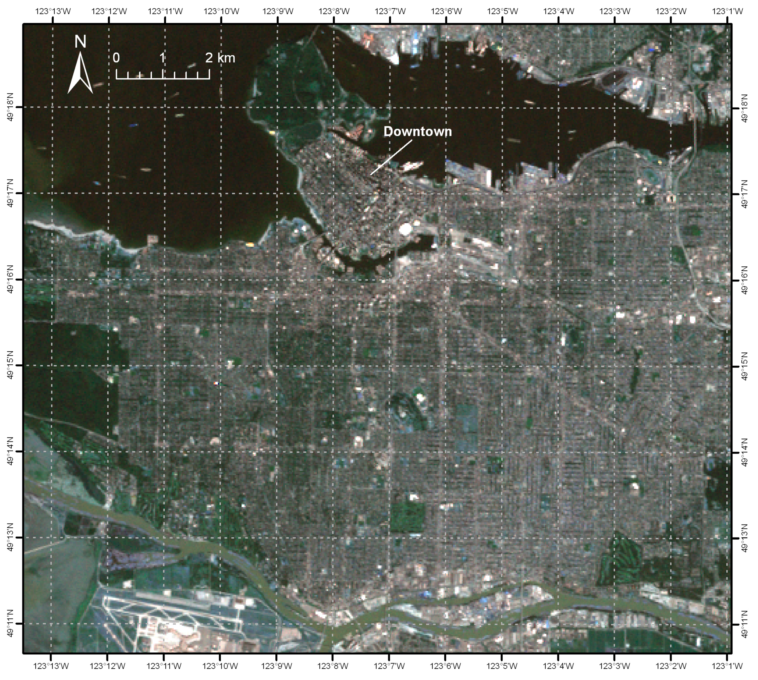
2.1.3. Validation Data

Lidar data for the city of Vancouver flown on 25 April 2013 were acquired as point-cloud data, and converted to 5 m first-return raster DSM in ENVI to match the calibration data.

2.2. Methods

Mapping of urban sky view factor was achieved in three main steps, outlined in Figure 2: (1) development of an empirical relationship between SP and SVF specific to the solar elevation of the Landsat data using the calibration data of the four US cities; (2) use of spectral mixture analysis to estimate per-pixel SP from the Landsat data; and (3) application of the empirical SP–SVF relationship to map SVF. The resulting SVF map was then validated using a SVF map derived from independent Lidar data.

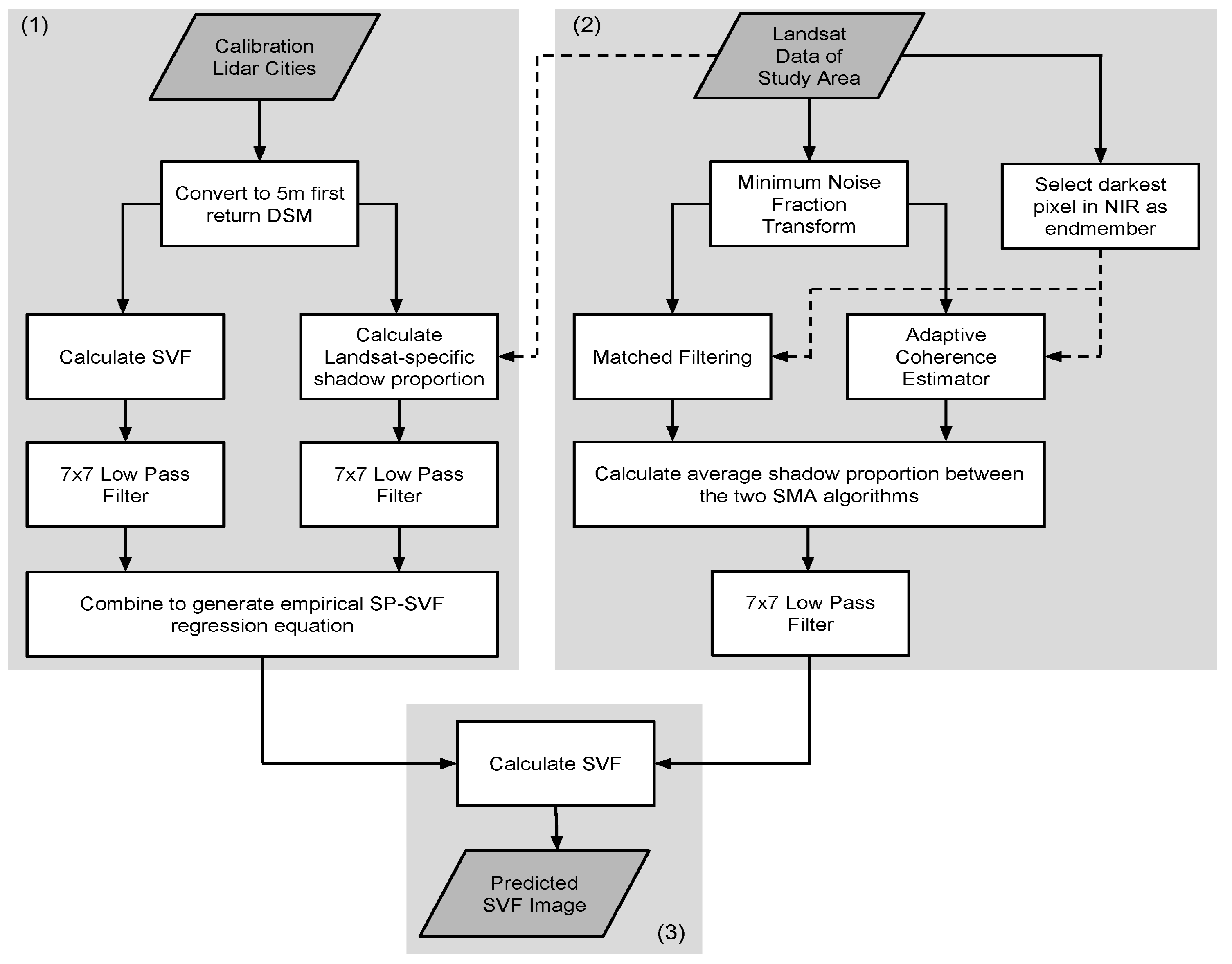
2.2.1. Development of Theoretical and Empirical Relationships between SP and SVF

To assess whether SVF could theoretically be predicted from SP and, if so, what kind of relationship would exist between the two variables, a synthetic 3D grid city with 30 m × 30 m buildings and 30 m wide streets was developed, similar to that used by Yuan and Chen [30] in a SVF modeling study. The synthetic city was built by creating a raster in an image manipulation program where a value of 0 represented street level, and a value of 1 represented buildings. Raster values could then be multiplied by a range of “building heights” to generate varying urban topography, and thus varying SVF and SP. For this city, SVF was determined at 1 m resolution using a SVF modeling program [31] that calculates the vertical angle to the horizon at a user specified scanning radius in a specified number of directions; in this case a radius of 500 m for 104 directions was used. SVF was calculated by averaging over an area with equal amounts of building, street, and intersection segments to eliminate any effect from the spatial offset between a structure and its shadow, and hence between SVF and SP, caused by the fact that structures cast shadows in one direction but reduce the SVF around them equally in all directions. SP was determined by modeling angles using the hillshade tool in ArcGIS 10 at 1 m resolution to create a binary shadow image. SP was then calculated as the proportion of 1 m shadowed elements to total 1 m elements within 30 m blocks of cells. SVF in the synthetic city was manipulated by varying the building heights, and the resulting SP was modeled for a number of solar elevations (20°, 40°, 60°, and 80°). For simplicity, solar azimuth was kept constant at 135°, close to the typical solar azimuth for mid-latitude Landsat data in the northern hemisphere. This modeling showed that a theoretical relationship between SVF and SP does exist, and that it follows a logarithmic pattern.

Lidar data from the four US cities were used to create SP–SVF relationships for real cities with a variety of street patterns, building heights, open spaces, etc., based on a solar elevation of 40° and solar azimuth of 135°. A solar elevation of 40° was chosen to minimize shadow saturation while still allowing small objects to cast detectable shadow. SP was determined using the same method as for the synthetic city, but a different approach was needed for SVF due to spatial variation in a real city’s SVF. In the northern mid-latitudes, structures cast shadows to the northwest during the mid-morning time of a Landsat overpass, but due to variations in building height as well as local topography, the spatial offset between SVF and SP is not easily quantified. In this study a 7 × 7 low pass filter was therefore applied to both the SVF derived using the Zakšek model [27], and SP, allowing a comparison between SP and the average SVF in the filtered area. Other filter sizes were also examined (3, 5, 7, 9, 11), and a trade-off between SVF prediction accuracy and spatial resolution was found to exist, for which the 7 × 7 filter was chosen as an acceptable compromise. For Landsat TM’s 30 m spatial resolution, the 7 × 7 filter extends between 105 m and 148 m from the central point, which is adequate to account for shadows cast by the majority of buildings in the cities used in this study when illuminated at a solar elevation of 40°, and still small enough to preserve some fine-scale spatial variations in urban SVF. The final SP-SVF relationship was determined by fitting a logarithmic curve to a combination of all four cities’ data points. A separate relationship was modeled for use with the Landsat data using the specific illumination angles present at image acquisition (elevation = 43.93°, azimuth = 152.02°). The resulting equation was used to calculate SVF from a SP map.

2.2.2. Estimation of SP and SVF

SP was determined using Spectral Mixture Analysis (SMA) of the Vancouver Landsat TM data. A Minimum Noise Fraction (MNF) transformation was first applied to the data to reduce sensor noise [32], with only the first three components being used in the analysis, the rest having been visually determined to contain mostly noise.

Partial unmixing methods were applied to the MNF components. Partial unmixing involves the use of only the target endmember, in this case shade, effectively reducing the mixture analysis to only two endmembers: “shadow” and “non-shadow”, thus removing the need to account for every surface type in a complicated urban environment. The shade endmember was selected by finding the darkest pixel in the Near Infrared (Landsat TM band 4) in our study area (excluding large water bodies). Band 4 was used to avoid the selection of shaded vegetation, as vegetation reflects strongly in this band.

Large water bodies were masked out using an existing landcover classification map of the region. The classification map was created using the CART classification tree algorithm, with spatial covariates including spectral indices such as NDVI and NDWI derived from Landsat TM data, and morphometric indices derived from a DEM. The model was trained and validated from points generated by a detailed manual inspection of high resolution imagery.

A number of partial unmixing methods were empirically examined in the study area, and two were chosen for their predictive qualities. Matched Filtering (MF) [33] and Adaptive Coherence Estimator (ACE) algorithms were chosen, as implemented in ENVI. In the empirical examination of the two methods using a sample Landsat and DSM dataset in the study area, it was found that MF generally slightly overestimated and ACE generally slightly underestimated SP. The average results from these two methods was found to provide an adequately accurate SP prediction, and used in the remaining analysis.

Upon applying a 7 × 7 Low Pass filter to the SP data to account for SP–SVF spatial offset, the data were converted to SVF using the empirical regression equation derived from the four US cities.

2.2.3. Validation

SP and SVF values used for validation were derived from the Vancouver Lidar data in the same way as for the four US cities, and smoothed using a 7 × 7 low pass filter to match the smoothed Landsat data. A stratified random sample of 1000 validation pixels were chosen from the study area, 500 each from manually identified high SVF and a low SVF regions. This subsampling was done to generate a balanced validation data set, as the vast majority of the study area is comprised of suburban housing, which has a high SVF, with only the downtown core containing low-SVF commercial towers.

3. Results

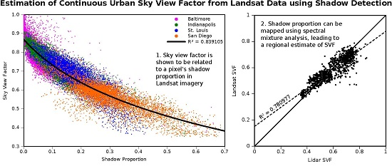
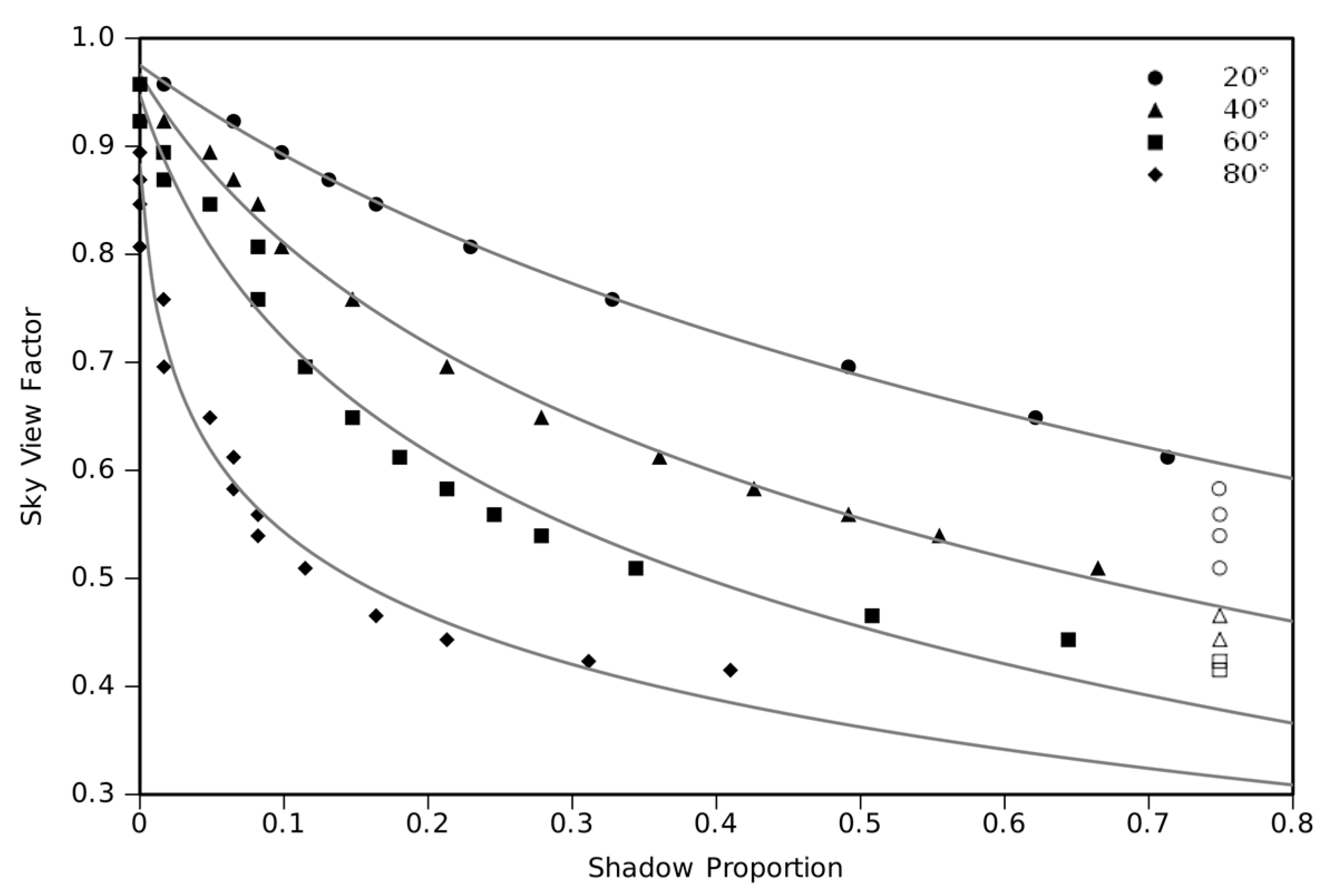
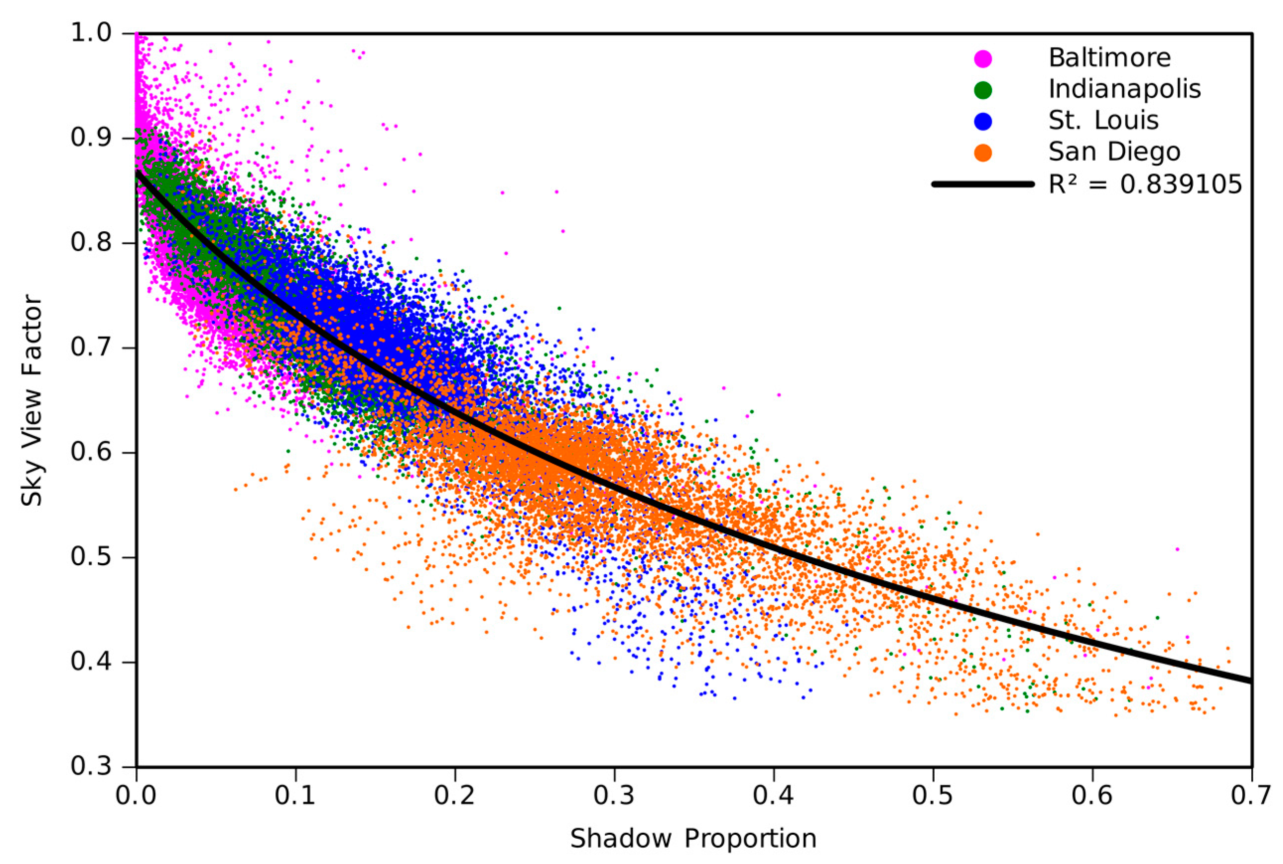
3.1. Development of an Empirical Relationship between SP and SVF

Theoretical modeling of SP and SVF in the synthetic city resulted in logarithmic relationships of the form SVF = a + b × ln(SP − c) and showed good fits that gradually decreased with increasing solar elevation (Figure 3). This decrease was due to resolution problems with ArcGIS’s hillshade tool causing multiple pairs of points to have identical SP values at different SVFs in the higher solar elevations. At high solar elevations, the change in SP for a particular change in SVF was very small compared to the same interval at low solar elevations. The hillshade tool was limited to a resolution of about 0.001 due to the method of resampling 1 m pixels into 30 m pixels, and thus very small changes in SP were not accurately quantified. At low solar elevations, a problem with shadow saturation was encountered, wherein a decrease in SVF would no longer correspond to an increase in SP because the area was already in full shade. This effect can be seen in Figure 3, where saturated points are represented by the shape outlines. The saturation point occurred at progressively lower SVFs as the solar elevation increased, however it always occurred at SP = 0.75, due to the averaging process and the city design, in which 75% of the city was “street level” and 25% was flat rooftops that are sunlit regardless of solar elevation. These results implied the existence of a range of moderate solar elevations for which the SP–SVF relationship could be best quantified; where solar elevation was high enough to prevent shadow saturation but low enough to ensure that SP changes for a given SVF change were large enough to be easily resolved. The ideal solar elevation needed to achieve this effect was determined to be approximately 40°.

The city simulation process resulted in evidence that there existed a good logarithmic relationship between SVF and SP, and revealed problems that might also be encountered when developing the relationship in real cities, namely problems with resolution and shadow saturation.

The logarithmic relationship between SP and SVF seen for the synthetic city was also evident for the four US cities (Figure 4), and a logarithmic function fit to their combined data points achieved a good fit (R² = 0.84). Shadow saturation was not a problem here because most of the shadow-casting structures were too small to cause saturation at 40° solar elevation. Where structures were large enough (mostly in San Diego), the local variations in building height meant that the rooftops of nearby lower buildings would accommodate the extra shade cast by taller building.

SVF in the four-cities model does not reach a maximum value of one, nor does it reach values close to zero as would be expected in a heavily built up area such as San Diego or downtown Indianapolis. SVF values in completely sunlit (SP = 0) pixels will not equal 1 because urban features will reduce SVF farther than their shadows are cast, thus a completely sunlit pixel may still experience a SVF reduction. Areas large enough for SVF to indeed equal 1 rarely occur in urban environments, meaning SP-SVF relationship at low SP values in Figure 4 can be considered accurate. The lack of very low SVF values is the result of a combination of the 30 m pixel size and spatial smoothing: most pixels in heavily built up areas will include elements from both streets (with low SVF values) and rooftops (with high SVF values).

The SP-SVF relationship modeled at the Landsat-specific illumination angle also resulted in good fit, with a slightly higher R² value than the four-cities model (R² = 0.85). The resulting equation, SVF = 0.330872 − 0.25827 × ln(SP + 0.13481), was used to calculate SVF in the Vancouver study area (see Section 4.3).

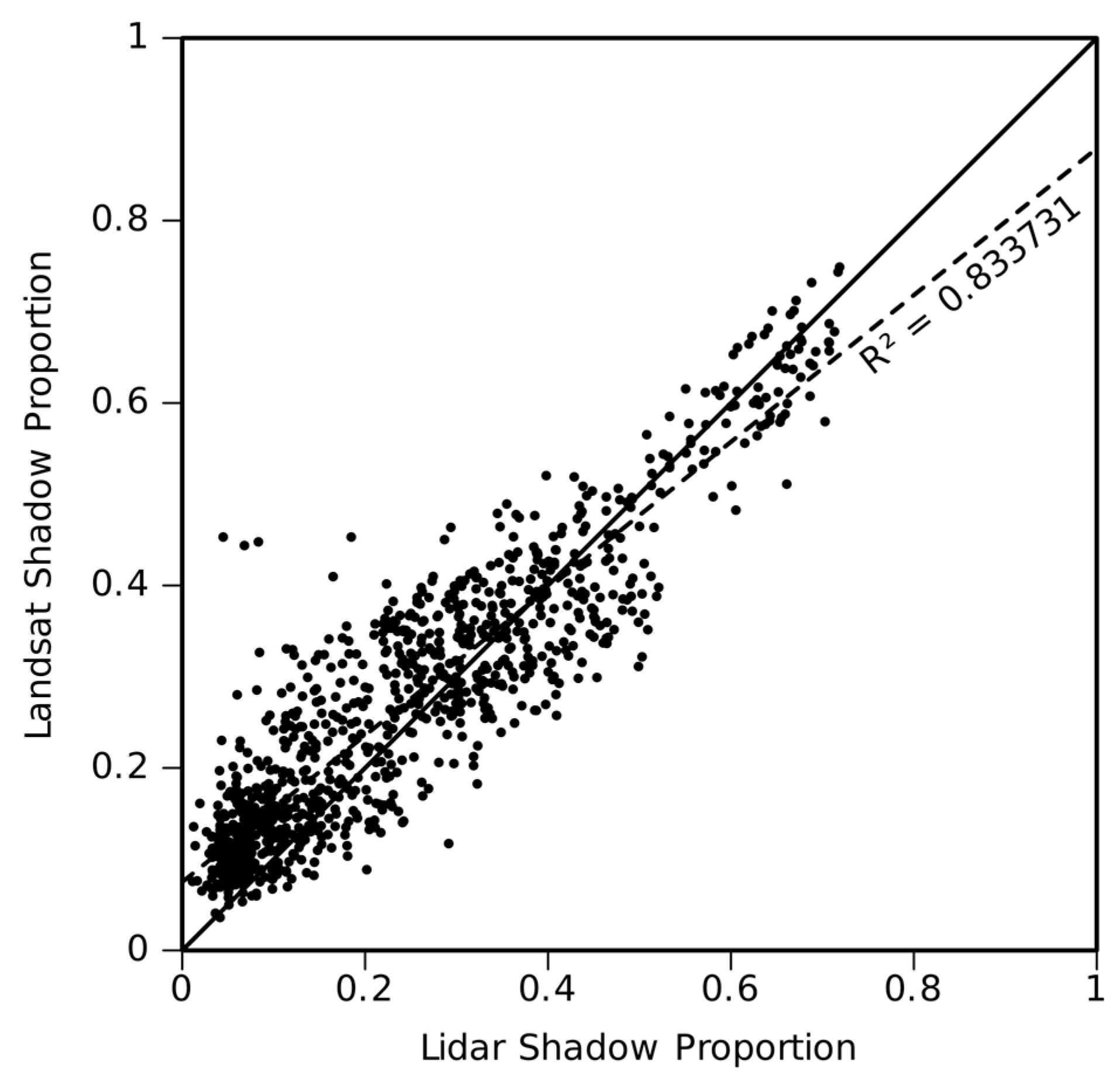
3.2. Estimation of SP

Selection of the darkest non-water pixel in Landsat band 4 resulted in a pixel in the downtown, low SVF region of Vancouver being used as the shadow endmember. Inspection using Lidar data from the area showed that the pixel was indeed located in a part of the city completely shaded by a large building, an ideal result.

Use of this endmember in both MF and ACE algorithms resulted in two SP images, with the MF image consistently underpredicting SP and ACE consistently overpredicting it. Averaging the results from the two individual algorithms led to a more accurate estimation of SP. When compared to SP validation data in Figure 5, the result shows good SP estimation, with an RMSE of 0.076 and an R² = 0.83. There is a very slight SP overprediction at low SP values, which should lead to a slight underprediction of SVF in high-SVF areas.

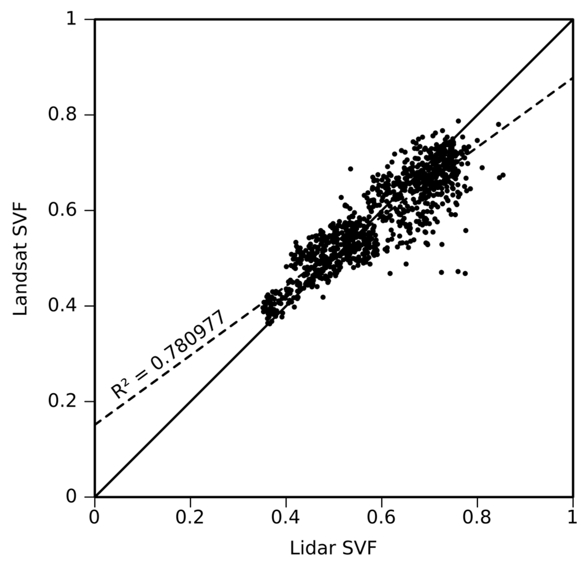
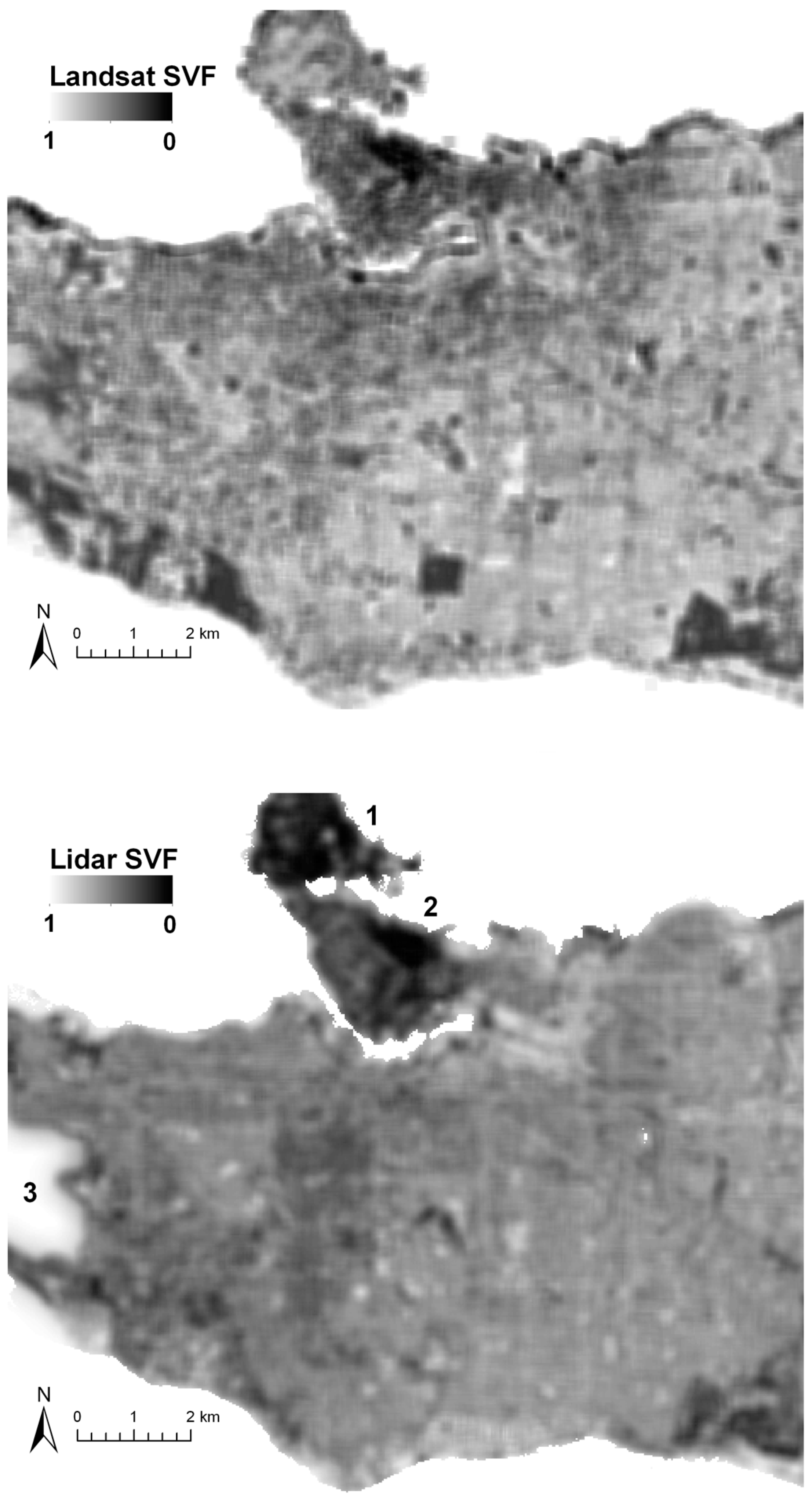
3.3. Sky View Factor Image and Validation

The calculation of SVF from the SP image resulted in an SVF prediction showing a good fit to validation data, with R² = 0.78 and an RMSE of 0.056 (Figure 6). As expected from examination of the SP data above, the model appears to slightly underpredict SVF in high SVF areas while slightly overpredicting in low SVF areas.

The Landsat-derived SVF map is shown in Figure 7 along with SVF derived from validation Lidar data. The model captures the broad spatial SVF pattern in the study area, with major zones of low and high SVF being readily identified. Downtown Vancouver (Annotation “2” in Figure 7) is correctly predicted to have a much lower SVF than the surrounding residential areas, while smaller variations in these residential areas are also evident. The generally lower SVF in the Eastern regions of Vancouver are correctly predicted, as well as areas of low SVF in the southeast caused by trees.

The large, obvious low-SVF square in south-central Vancouver, as well as smaller scattered patches are possibly the result of a discrepancy in scale between the Landsat shadow detection and the Lidar SVF calculations, where very small shadows such as those cast by individual blades of grass are not represented in the 5 m cell size from which the Lidar SVF is calculated. This issue and a possible solution are discussed in greater detail below.

4. Discussion

4.1. Model Limitations

The key limitation for this SVF mapping method is the difference between the very small scale on which shadow and SVF reduction occurs, and the relatively larger scale that is relevant for SVF application in energy balance models, an issue best illustrated by the prediction of very low SVF over grass fields that is evident in Figure 7. Many small shadows cast by shrubs or large blades of grass may cause a grassy area to contain a high proportion of shadow, which would produce a Landsat prediction of low SVF for that area. However, at the metre scale that is typical of urban energy balance models, a similar scale to that of typical Lidar data (including our validation data), such small shadows would remain undetected. This problem can be solved by identifying grassland areas using a landcover classification and either applying a correction factor or assigning them a predetermined value (as was done for the ocean), though such reclassification was not done here in the interest of clarity.

Another important limitation is the inability of the model to predict SVF over water. This is caused by the spectral similarity between water and shaded urban areas, leading water to be identified as shade and thus leading to incorrect predictions of extremely low SVF on water. This issue can be resolved by identifying large water bodies using a landcover classification and replacing SVF values over water with either a constant value, as done in our study, or with values calculated using a bare-earth DEM to account for the reduction of SVF near shore.

A third limitation for this approach to Landsat-based SVF mapping is the necessity of the modeled city to be on relatively flat ground. Extreme topography will generate its own shadows, and even moderate topography will alter the length of shadows for a given value of SVF, thus changing the established SP–SVF regression. As the majority of the world’s large cities are not located in areas of dramatic terrain, this limitation does not greatly affect its general applicability, although it should be kept in mind if application for cities in mountainous regions is considered.

4.2. Applicability of the Method to Cities Worldwide

These methods have been developed using only cities with a grid layout where streets generally run North-South and East-West. Grid cities are typical of North America, but cities elsewhere may follow a much less regular pattern. The general approach outlined in this study is likely to also work in cities with less regular street patterns, although the modeling of a separate SP-SVF relationship using Lidar data from a group of such cities will likely be required.

4.3. Use of a Synthetic City for Calibration

Using a synthetic city to model the SP-SVF relationship instead of multiple sets of Lidar data was attempted as a part of this study, though the results were unsatisfactory. Many varieties of regular grid cities were examined for their representability of real-world cities, including cities with varying street-to-building width ratios and varying building sizes, but these all showed poor results by not closely corresponding to the empirical relationship from real cities shown in Figure 4. This suggests that the SP–SVF relationship is influenced by the complex structural heterogeneity of real cities, which includes a range of street orientations, widths and shapes as well as local variations in building heights. Future research may find that a particular synthetic city design is better suited for equation calibration, or even that it would be possible to select a particular city type, for example to differentiate between North American and European style cities.

4.4. Potential Application

With increasing availability of Lidar data for many cities, from which accurate urban structure metrics including SVF can be derived, the need for a Landsat-based SVF mapping algorithm may seem small. We suggest three scenarios in which our algorithm is likely to provide the best available solution to SVF mapping. (1) Lidar data are still not available for many cities worldwide, or may be available only at a cost that makes them effectively inaccessible for a range of users while Landsat data are freely available for download; (2) Where Lidar data are freely available, they are unlikely to provide complete coverage of an extensive metropolitan area. Where such an area is the entity under study, Lidar- and Landsat-derived SVF maps may be combined to ensure complete coverage; (3) Any analysis of long-term change in urban structure must rely on temporally consistent and spatially extensive data sets. The Landsat image archive, with acquisitions by TM/ETM+/OLI sensors going back to 1984, provides three decades of freely available and spatially and spectrally consistent data, from which analyses of urban structure changes may be performed using our approach. In these three scenarios, there is currently no alternative approach for a spatially complete derivation of SVF.

Since the SVF data are derived from 30 m Landsat pixels, they are of a coarse resolution, being able to identify large-scale variation across cities and large metropolitan areas, but are unable to resolve intra- and inter-street scale SVF variations. As a result, appropriate applications will typically involve its use in macro-scale urban studies that investigate climate variability across these large scales. An example of such an application can be seen in its use as a data layer in a statistical model to estimate the daily maximum air temperature [34] in the Greater Vancouver Area. By including the SVF data along with other predictors in this regression model, the mean absolute errors of predictions for validation locations were reduced from 1.89 °C to 1.82 °C, with relatively greater improvement in densely built up areas that were poorly predicted without the SVF layer. In addition, permutation-based variable importance measures [35,36,37], which quantify the increase in prediction errors when a predictor is permuted in the validation data, suggest that the contribution of the SVF data layer to predictions made by the model is greater than that of other more commonly used predictors, such as vegetation liquid water and elevation. This provides a tangible example of the importance of SVF for the urban radiation and energy balance. Hemispherical photography and airborne Lidar methods, though able to generate SVF data with greater accuracy and at higher spatial resolution, have not been able to generate complete and continuous coverage of SVF data for a large urban environment, as is necessary for most mapping exercises. The approach described in this paper, which is based on freely available Landsat data, is the first that enables generation of such continuous coverage.

5. Conclusions

Analytical methods for calculating continuous sky-view factor (SVF) maps using 3D structural data have become commonplace, however 3D data can be expensive or difficult to acquire, resulting in many urban areas requiring the labour-intensive gathering of field-based point data. This study developed a method for producing spatially continuous SVF estimates from Landsat imagery based on the principle that shadows are cast by the same buildings that obscure the sky from view and thus reduce SVF. We first confirmed the existence of a logarithmic relationship between shadow proportion (SP) and SVF through simulations using a synthetic grid city, which, when artificially illuminated, allowed us to investigate SP and SVF values as they vary with changing sun elevation and building heights, and then derived an empirical logarithmic relationship between SP and SVF for real cities, calibrated using Lidar data from four US cities. We then estimated SP using the averaged result from two partial unmixing approaches, Matched Filtering and Adaptive Coherence Estimation, applied to Landsat 5 TM data from Vancouver, Canada. Both approaches effectively simplify target endmembers to “shadow” and “non-shadow” and thus eliminate the need to define many endmembers for the complicated urban landcover in the area. The shadow endmember was automatically defined as the darkest non-water pixel in Near Infrared (Landsat band 4). The resulting SP estimates closely matched SP values derived from independent validation Lidar data covering areas with a range of urban structures (RMSE = 0.076, R² = 0.83). Finally, we applied the empirical SP-SVF relationship to the SP estimates to produce per-pixel estimates of SVF for Vancouver. These Landsat-based SVF estimates also closely matched SVF values derived from the Lidar data (RMSE = 0.056, R² = 0.78). We suggest that the methodology described and validated in our study may be the best approach to generate spatially complete information on sky-view factor in urban environments whenever Lidar data are unavailable or their coverage is spatially or temporally incomplete.

References

1. Arnfield, A.J. Two decades of urban climate research: A review of turbulence, exchanges of energy and water, and the Urban Heat Island. Int. J. Climatol. 2003, 23, 1–26. [Google Scholar] [CrossRef]
2. Tan, J.; Zheng, Y.; Tang, X.; Guo, C.; Li, L.; Song, G.; Zhen, X.; Yuan, D.; Kalkstein, A.J.; Li, F.; et al. The Urban Heat Island and its impact on heat waves and human health in Shanghai. Int. J. Biometeorol. 2010, 54, 75–84. [Google Scholar] [CrossRef] [PubMed]
3. Shahmohamadi, P.; Che-Ani, A.I.; Etessam, I.; Maulud, K.N.A.; Tawil, N.M. Healthy environment: The need to mitigate Urban Heat Island effects on human health. Proc. Eng. 2011, 20, 61–70. [Google Scholar] [CrossRef]
4. Watson, I.D.; Johnson, G.T. Short communication: Graphical estimation of Sky View-Factors in urban environments. J. Climatol. 1987, 7, 193–197. [Google Scholar] [CrossRef]
5. Oke, T.R. Street design and urban canopy layer climate. Energy Build. 1988, 11, 103–113. [Google Scholar] [CrossRef]
6. Oke, T.R. Canyon geometry and the nocturnal Urban Heat Island: Comparison of scale model and field observations. J. Climatol. 1981, 1, 237–254. [Google Scholar] [CrossRef]
7. Oke, T.R.; Johnson, G.T.; Steyn, D.G.; Watson, I.D. Simulation of surface urban heat islands under ‘ideal’ conditions at night. Part 2: Diagnosis of causation. Bound. Layer Meteorol. 1991, 56, 339–358. [Google Scholar] [CrossRef]
8. Holmer, B. A simple operative method for determination of Sky View Factors in complex urban canyons from fisheye photographs. Meteorol. Z. 1992, 1, 236–239. [Google Scholar]
9. Nunez, M.; Eliasson, I.; Lindgren, J. Spatial variations of incoming longwave radiation in Goteborg, Sweden. Theor. Appl. Climatol. 2000, 67, 181–192. [Google Scholar] [CrossRef]
10. Svensson, M.K. Sky View Factor analysis—Implications for urban air temperature differences. Meteorol. Appl. 2004, 11, 201–211. [Google Scholar] [CrossRef]
11. Erell, E.; Williamson, T. Intra-urban differences in canopy layer air temperature at a mid-latitude city. Int. J. Climatol. 2007, 27, 1243–1255. [Google Scholar] [CrossRef]
12. Gál, T.; Lindberg, F.; Unger, J. Computing continuous Sky View Factors using 3D urban raster and vector databases: Comparison and application to urban climate. Theor. Appl. Climatol. 2009, 95, 111–123. [Google Scholar] [CrossRef]
13. Scarano, M.; Sobrino, J.A. On the relationship between the Sky View Factor and the land surface temperature derived by Landsat-8 images in Bari, Italy. Int. J. Remote Sens. 2015, 36, 4820–4835. [Google Scholar] [CrossRef]
14. Steyn, D.G. The calculation of view factors from fisheye-lens photographs. Atmos. Ocean 1980, 18, 254–258. [Google Scholar] [CrossRef]
15. Grimmond, C.S.B.; Potter, S.K.; Zutter, H.N.; Souch, C. Rapid methods to estimate sky-view factors applied to urban areas. Int. J. Climatol. 2001, 21, 903–913. [Google Scholar] [CrossRef]
16. Chapman, L.; Thornes, J.E. Real-time sky-view factor calculation and approximation. J. Atmos. Ocean. Technol. 2004, 21, 730–741. [Google Scholar] [CrossRef]
17. Debbage, N. Sky-view factor estimation: A case study of Athens, Georgia. Geogr. Bull. 2013, 54, 49–57. [Google Scholar]
18. Kidd, C.; Chapman, L. Derivation of sky-view factors from Lidar data. Int. J. Remote Sens. 2012, 33, 3640–3652. [Google Scholar] [CrossRef]
19. Yang, J.; Wong, M.S.; Meneti, M.; Nichol, J. Modeling the effective emissivity of the urban canopy using Sky View Factor. ISPRS J. Photogramm. Remote Sens. 2015, 105, 211–219. [Google Scholar] [CrossRef]
20. Chen, L.; Ng, E.; An, X.; Ren, C.; Lee, M.; Wang, U.; He, Z. Sky View Factor analysis of street canyons and its implications for daytime intra-urban air temperature differentials in high-rise, high-density urban areas of Hong Kong: A GIS-based simulation approach. Int. J. Climatol. 2012, 32, 121–136. [Google Scholar] [CrossRef]
21. An, S.M.; Kim, B.S.; Lee, H.Y.; Kim, C.H.; Yi, C.Y.; Eum, J.H.; Woo, J.H. Three-dimensional cloud based Sky View Factor analysis in complex urban settings. Int. J. Remote Sens. 2014, 34, 2685–2701. [Google Scholar] [CrossRef]
22. Su, J.G.; Brauer, M.; Buzzelli, M. Estimating urban morphometry at the neighborhood scale for improvement in modeling long-term average air pollution concentrations. Atmos. Environ. 2008, 42, 7884–7893. [Google Scholar] [CrossRef]
23. Dare, P.M. Shadow analysis in high-resolution satellite imagery of urban areas. Photogramm. Eng. Remote Sens. 2005, 71, 169–177. [Google Scholar] [CrossRef]
24. Luo, H.; Shao, Z. A shadow detection method from urban high resolution remote sensing image based on color features of shadow. In Proceedings of the 2012 International Symposium on Information Science and Engineering (ISISE), Shanghai, China, 14–16 December 2012.
25. Shao, Y.; Taff, G.N.; Walsh, S.J. Shadow detection and building-height estimation using IKONOS data. Int. J. Remote Sens. 2011, 32, 6929–6944. [Google Scholar] [CrossRef]
26. Shimabukuro, Y.E.; Haertel, V.F.A.; Smith, J.A. Landsat Derived Shade Images of Forested Areas. Proc. ISPRS 1988, 27, 534–543. [Google Scholar]
27. Ridd, M.K. Exploring a V-I-S (vegetation-impervious surface-soil) model for urban ecosystem analysis through remote sensing: Comparative anatomy for cities. Int. J. Remote Sens. 1995, 16, 2165–2185. [Google Scholar] [CrossRef]
28. Small, C. Comparative analysis of urban reflectance and surface temperature. Remote Sens. Environ. 2006, 104, 168–189. [Google Scholar] [CrossRef]
29. Lu, D.; Weng, Q. Spectral Mixture Analysis of the urban landscape in Indianapolis with Landsat ETM+ imagery. Photogramm. Eng. Remote Sens. 2004, 70, 1053–1062. [Google Scholar] [CrossRef]
30. Yuan, C.; Chen, L. Mitigating Urban Heat Island effects in high-density cities based on Sky View Factor and urban morphological understanding. Archit. Sci. Rev. 2011, 54, 305–315. [Google Scholar] [CrossRef]
31. Zakšek, K.; Oštir, K.; Kokalj, Ž. Sky-View Factor as a relief visualization technique. Remote Sens. 2011, 3, 398–415. [Google Scholar] [CrossRef]
32. Green, A.A.; Berman, M.; Switzer, P.; Craig, M.D. A transformation for ordering multispectral data in terms of image quality with implications for noise removal. IEEE Trans. Geosci. Remote Sens. 1988, 26, 65–74. [Google Scholar] [CrossRef]
33. Kuenzer, C.; Bachmann, M.; Mueller, A.; Lieckfeld, L.; Wagner, W. Partial unmixing as a tool for single surface class detection and time series analysis. Int. J. Remote Sens. 2008, 29, 3233–3255. [Google Scholar] [CrossRef]
34. Ho, H.C.; Knudby, A.; Sirovyak, P.; Xu, Y.; Hodul, M.; Henderson, S.B. Mapping maximum urban air temperature on hot summer days. Remote Sens. Environ. 2014, 154, 38–45. [Google Scholar] [CrossRef]
35. Strobl, C.; Malley, J.; Tutz, G. An introduction to recursive partitioning: Rationale, application, and characteristics of classification and regression trees, bagging, and random forests. Phys. Methods 2009. [Google Scholar] [CrossRef] [PubMed] [Green Version]
36. Genuer, R.; Poggi, J.M.; Tuleau-Malot, C. Variable selection using random forests. Pattern Recognit. Lett. 2010, 31, 2225–2236. [Google Scholar] [CrossRef]
37. Knudby, A.; LeDrew, E.; Brenning, A. Predictive mapping of reef fish species richness, diversity and biomass in Zanzibar using IKONOS imagery and machine-learning techniques. Remote Sens. Environ. 2010, 114, 1230–1241. [Google Scholar] [CrossRef]
Figure 1. Landsat true colour image of the study area, Vancouver, BC, Canada.
Remotesensing 08 00568 g001
Figure 2. Overview of the modeling process to estimate sky view factor (SVF) from Landsat imagery. Shaded regions correspond to numbered steps described in Section 3.
Remotesensing 08 00568 g002
Figure 3. Shadow proportion-sky view factor (SP-SVF) relationship in 30 m × 30 m grid city at various solar elevations, and 135° solar azimuth. Building heights of 1, 2, 3, 4, 5, 7, 10, 15, 20, 25, 30, 35, 40, 50, 75, 100, 150, and 200 m were used to vary SVF. The SP-SVF relationship appears to be a nearly perfect logarithmic relationship, with fit accuracy falling slightly in higher solar elevations. Points with saturated SP are shown as shape outlines and are not used for calculating trendlines. Pairs of points at 60° and 80° that appear to have identical SP values despite having different SVF result from the hillshade tool being unable to resolve such small changes in SVF into differing SP values.
Remotesensing 08 00568 g003
Figure 4. Scatter plot of shadow proportion-sky view factor (SP-SVF) relationships in four US cities modeled at 40° solar elevation and 135° solar azimuth. A log curve is fit to a combination of all data points, resulting in a good fit similar to that of the synthetic city.
Remotesensing 08 00568 g004
Figure 5. Accuracy of shadow proportion (SP) values predicted using an average of results from Matched Filtering and Adaptive Coherence Estimator SMA algorithms, as compared to SP values derived analytically from Lidar artificially illuminated at the Vancouver Landsat data’s solar elevation and azimuth conditions. SP is well predicted, with an RMSE of 0.076 and an R2 = 0.83, though there exists a slight overprediction at low SP values. Highly overpredicted outliers are pixels representing grass fields; the cause if this is discussed in Section 5.
Remotesensing 08 00568 g005
Figure 6. Accuracy of the predicted sky view factor (SVF) values as compared to SVF derived analytically from Lidar data. SVF is well predicted, with an RMSE of 0.056 and an R2 = 0.78, These data correspond to the SVF images shown in Figure 7, using the darkest pixel in NIR Landsat band 4 in the Spectral Mixture Analysis.
Remotesensing 08 00568 g006
Figure 7. The resulting sky view factor (SVF) image (top) compared with the validation data Lidar SVF image (bottom). The ocean has been masked out of the image and replaced with a SVF value of 1, representing the flat ocean surface, as the model performs poorly over water. The large dark (low-SVF) patches in the predicted data are the result of shadow casting and SVF reduction by grass and short shrubs on a smaller scale than is visible on the Lidar data.
Remotesensing 08 00568 g007