Automated Subpixel Surface Water Mapping from Heterogeneous Urban Environments Using Landsat 8 OLI Imagery

Abstract

Water bodies are a fundamental element of urban ecosystems, and water mapping is critical for urban and landscape planning and management. Remote sensing has increasingly been used for water mapping in rural areas; however, when applied to urban areas, this spatially- explicit approach is a challenging task due to the fact that the water bodies are often of a small size and spectral confusion is common between water and the complex features in the urban environment. Water indexes are the most common method of water extraction at the pixel level. More recently, spectral mixture analysis (SMA) has been widely employed in analyzing the urban environment at the subpixel level. The objective of this study is to develop an automatic subpixel water mapping method (ASWM) which can achieve a high accuracy in urban areas. Specifically, we first apply a water index for the automatic extraction of mixed land-water pixels, and the pure water pixels that are generated in this process are exported as the final result. Secondly, the SMA technique is applied to the mixed land-water pixels for water abundance estimation. As for obtaining the most representative endmembers, we propose an adaptive iterative endmember selection method based on the spatial similarity of adjacent ground surfaces. One classical water index method (the modified normalized difference water index (MNDWI)), a pixel-level target detection method (constrained energy minimization (CEM)), and two widely used SMA methods (fully constrained least squares (FCLS) and multiple endmember spectral mixture analysis (MESMA)) were chosen for the water mapping comparison in the experiments. The results indicate that the proposed ASWM was able to detect water pixels more efficiency than other unsupervised water extraction methods, and the water fractions estimated by the proposed ASWM method correspond closely to the reference fractions with the slopes of 0.97, 1.02, 1.04, and 0.98 and the R-squared values of 0.9454, 0.9486, 0.9665, and 0.9607 in regression analysis corresponding to different test regions. In the quantitative accuracy assessment, the ASWM method shows the best performance in water mapping with the mean kappa coefficient of 0.862, mean producer’s accuracy of 82.8%, and mean user’s accuracy of 91.8% for test regions.

1. Introduction

Remote sensing has played an important role in various water studies, including flood monitoring [1], water resource estimation [2,3], water quality assessment [4,5], and shoreline/coastline extraction [6,7]. All of these applications are closely related to surface water mapping from remote sensing images.

Optical remote sensing of water bodies is based on the difference in the spectral reflectance of land and water. Water absorbs most of the energy in the near-infrared and middle-infrared wavelengths, whereas other surface materials have a higher reflectance in these wavelengths. To date, various water body extraction algorithms for optical imagery have been developed, and they can be categorized into four basic types: (1) hard classification [8,9]; (2) single-band thresholding [10,11]; (3) spectral water indexes [12,13,14,15,16]; and (4) spectral unmixing [17,18,19]. The hard classification method can achieve high precision in the water extraction, however, its algorithm is always complicated and time-consuming. Single-band thresholding is the simplest water extraction method, it mainly depends on the reflectivity difference of water and others in the infrared wave bands, and it can achieve high precision in most cases. The two-band spectral water index method has the dual advantages of simplicity and high precision; it is the most frequently used method for water extraction. Among these methods, the first three groups of methods can only obtain water maps at the pixel level, which may not meet the precise requirements of the practical applications in urban areas.

The spectral mixture analysis (SMA) can be used as a pre-processing step for water mapping at sub-pixel resolution. Reliable SMA is critical for the post-sub-pixel mapping process [20,21]. However, the typical processes of SMA consist of two steps—endmember determination and abundance estimation [22]—and for each step, prior knowledge or manual intervention is usually required [23,24,25]. As all of the land-cover types are usually involved in a SMA analysis, this is too complicated when surface water is the only land-cover type of concern. Several previous studies have simplified the SMA process for subpixel water mapping, e.g., Sun et al. [26], and Ma et al. [27] proposed subpixel water mapping methods based on MODIS 250-m data using a linear mixture model, and Pardo-Pascual et al. [7] used the single-band intensity gradient to determine the shoreline position at a subpixel precision. Sethre et al. [28] applied the IMAGINE Subpixel Classifier [29] to detect subpixel-scale ponds.

Even though several subpixel-level water body extraction methods have been proposed in the literature, the research for urban regions is still few and the existing methods seem ineffective for urban regions. In the highly heterogeneous urban environments, the water bodies, like narrow rivers and small ponds, are distributed sparsely in a subpixel-scale size, and water extraction methods often fail to distinguish the narrow rivers in urban areas because the mixed land-water pixels are defined by the neighborhoods of the pure water pixels. The large amount of low albedo surfaces and building shadows, which are easily confused with water bodies in urban areas, also bring a big challenge to urban subpixel water mapping.

In this paper, an automatic subpixel water mapping method (ASWM) was introduced for use in urban areas using Landsat 8 OLI data. The objectives of this research are: (1) to develop an automatic mixed land-water pixel extraction technique utilizing a water index; (2) to derive the most representative endmembers of both water and land by utilizing neighboring water pixels and the optimal neighboring land pixels, respectively; and (3) to apply a linear unmixing model for subpixel water fraction estimation.

The organization of this paper is structured as follows: Section 2 introduces the study areas and datasets. Section 3 describes the proposed ASWM method in detail, including automated mixed land-water pixel extraction, representative endmember selection, and water abundance estimation by a linear unmixing method. In Section 4, the Landsat OLI data used in the experiments were described, and the surface water mapping results and quantitative accuracy assessment are given. Finally, a discussion and the conclusions are presented in Section 5 and Section 6, respectively.

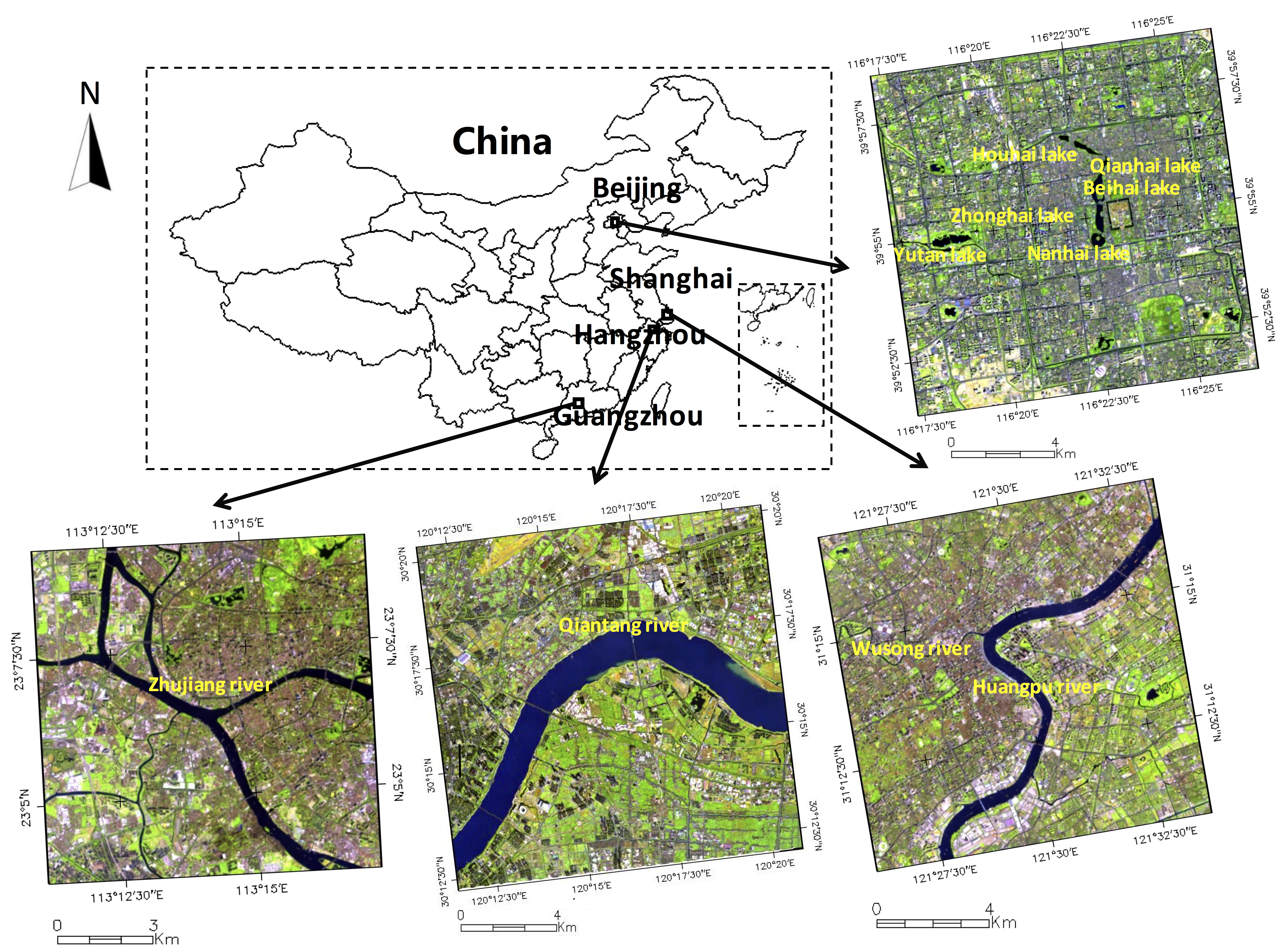
2. Study Areas and Data Sources

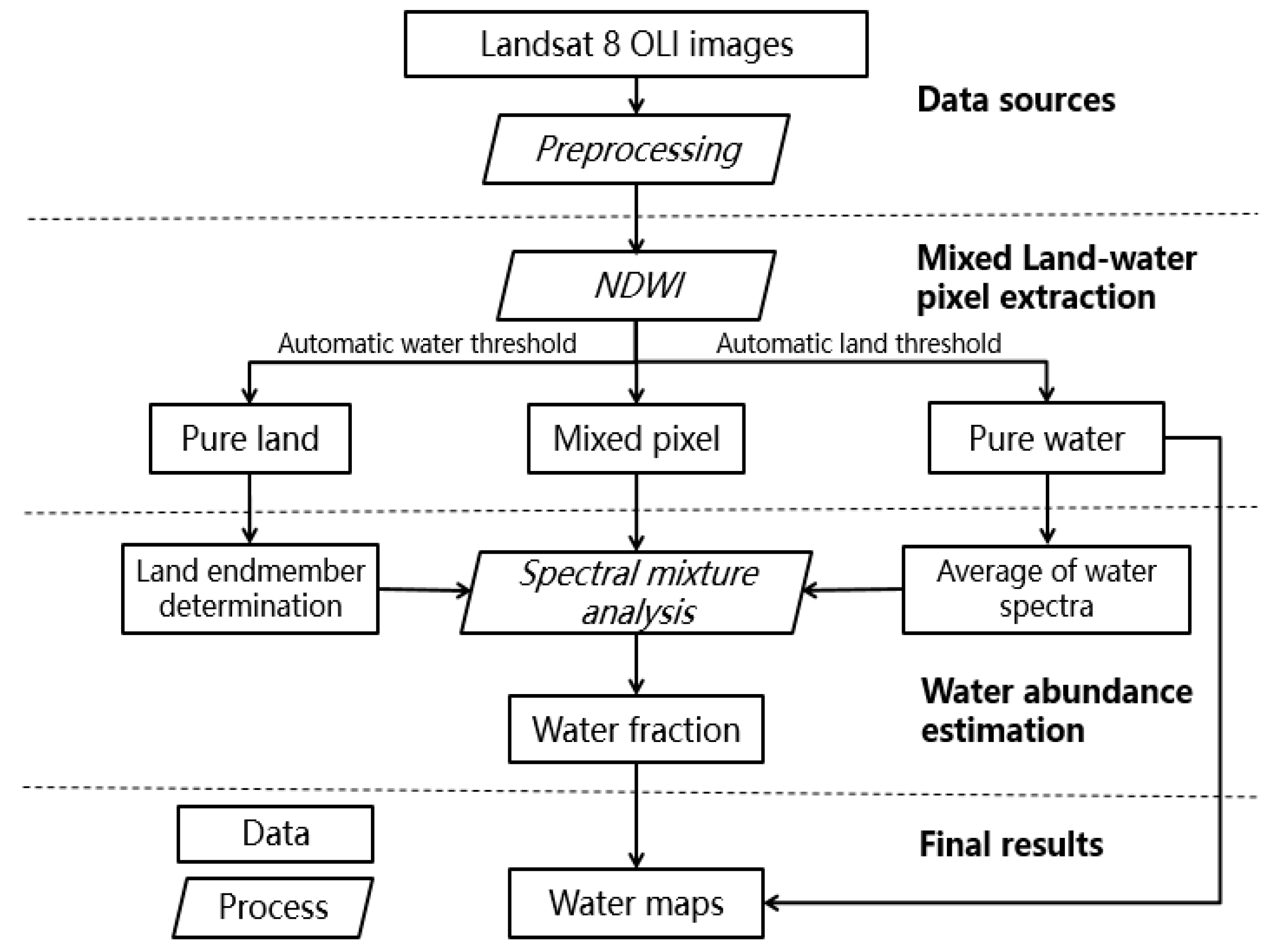
Four different cities in China were selected as study areas in order to include diverse water body types and complex ground surface features. The selected cities were Beijing, Shanghai, Hangzhou, and Guangzhou (see Figure 1). Beijing is the capital of China and has the second-largest population of any city in China, just behind Shanghai. The selected scene is located in the center of Beijing. The surface water bodies in this area are mostly clear water present as artificial lakes, ponds, and small rivers. The Shanghai scene is located at Lujiazui, the city center of Shanghai, where the Huangpu River and its small tributaries surround the area. In this area, it is difficult to distinguish the water bodies because of the shadows caused by the high-rise buildings. The selected Hangzhou scene is located in the suburbs of the city, where there are abundant water bodies, including the Qiantang River (which varies from clear to turbid) and its tributaries, and many small ponds. The Guangzhou scene is surrounded by the Pearl River and its tributaries, and this area can be roughly divided into half urban and half suburban areas. The water bodies in this area are of great diversity. The details of the study areas and the corresponding Landsat 8 OLI images are summarized and listed in

Table 1. Details of the study areas.

Study Area	Main Water Bodies (km2)	Water Characteristics	Acquisition Date of OLI Image	Acquisition Date of Reference Data
Beijing	Nanhai Lake (0.20)	Small and clear lakes	16 April 2015	13 April 2015
	Zhonghai Lake (0.25)
	Beihai Lake (0.35)
	Qianhai Lake (0.08)	Small and clear rivers
	Houhai Lake (0.16)
	Yutan Lake (0.40)
Shanghai	Huangpu River (7.61)	Moderately turbid river	10 April 2014	25 November 2014
	Wusong River (0.38)	Small and clear lake		22 November 2014
Hangzhou	Qiantang River (28.75)	Clear lake	13 Decemebr 2014	24 December 2014
		Moderately turbid and turbid river		3 May 2014
Guangzhou	Pearl River (7.47)	Clear and moderately turbid river	15 October 2014	5 October 2014

.

All of the OLI images used in this study were free of clouds, and atmospheric correction using the Fast Line-of-sight Atmospheric Analysis of Spectral Hypercubes (FLAASH) module was applied to all of the selected scenes. The coastal/aerosol band (band 1 of OLI) and the cirrus band (band 9 of OLI), which include little information under cloudless conditions, were removed and the remaining six bands were used in the experiments. To obtain the reference data (true water fraction of each pixel), fine spatial resolution images (<1 m) were acquired from Google Earth^TM. The acquisition dates between the Google Earth^TM images and the test images could be considered to be closely matched, since the water bodies in urban areas are usually stable over a short time period, so the slight bias of the surface water boundaries between the reference data and test images could be ignored. The “true” boundaries of all the water bodies in the study areas were digitized manually on-screen and used for the accuracy assessment of the water body subpixel mapping. The OLI images were registered to the reference images using a first order polynomial with at least 20 ground control points in each scene, with root-mean-square errors (RMSEs) of 0.23, 0.3, 0.22, and 0.29 pixels, corresponding to the test sites of Beijing, Shanghai, Hangzhou, and Guangzhou, respectively.

3. Methodology

The ASWM approach can be divided into three major steps: (1) automated mixed land-water pixel extraction; (2) determination of endmember spectra from neighboring pixels; and (3) linear SMA with the endmember spectra, and the detailed process is shown in the flowchart of the ASWM approach (see Figure 2).

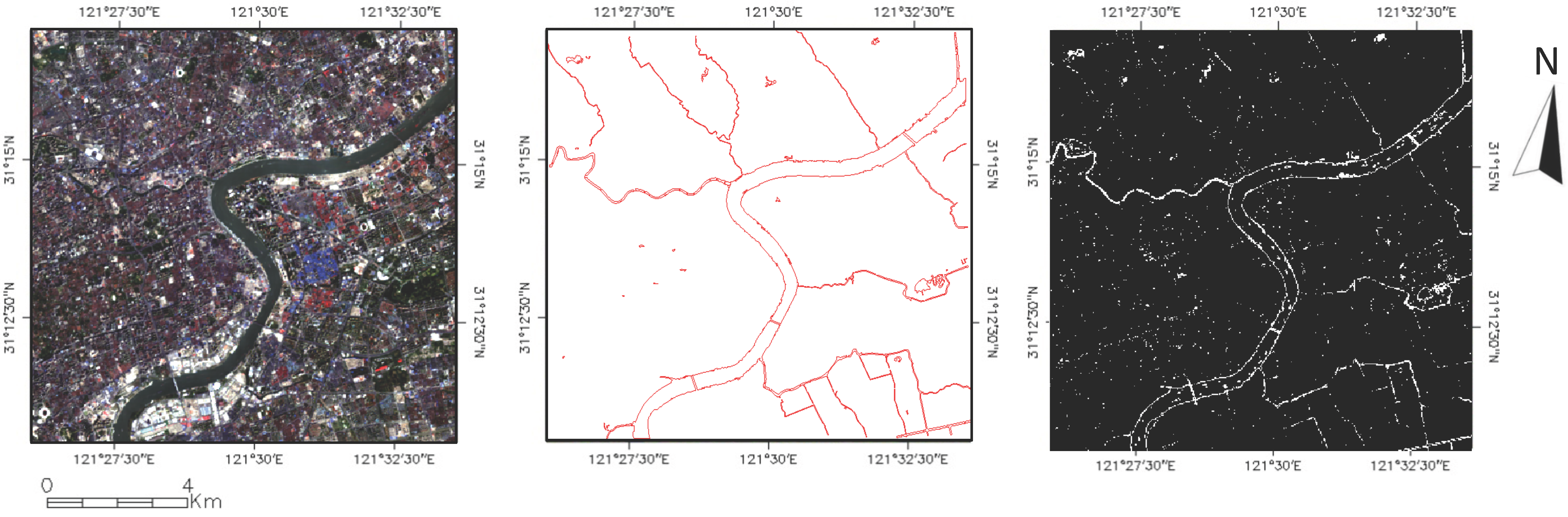
3.1. Automatic Mixed Land-Water Pixel Extraction

3.1.1. Normalized Difference Water Index (NDWI) Calculation

The NDWI is a quantitative spectral indicator designed for characterizing water bodies [12,13]. It has been widely used for water body extraction through enhancing the water information while suppressing the land information in remote sensing imagery [30]. In this study, the NDWI is used for obtaining the mixed land-water pixels through identifying those pixels which are neither enhanced nor suppressed. A previous study showed that, for Landsat 8 OLI images, the green band and short-wave infrared band 2 (SWIR-2) are the best option to calculate the NDWI [31].

$$NDWI=\frac{{\rho }_{Green}-{\rho }_{SWIR2}}{{\rho }_{Green}+{\rho }_{SWIR2}},$$

(1)

where ${\rho }_{Green}$ and ${\rho }_{SWIR2}$ are the reflectance of the respective bands.

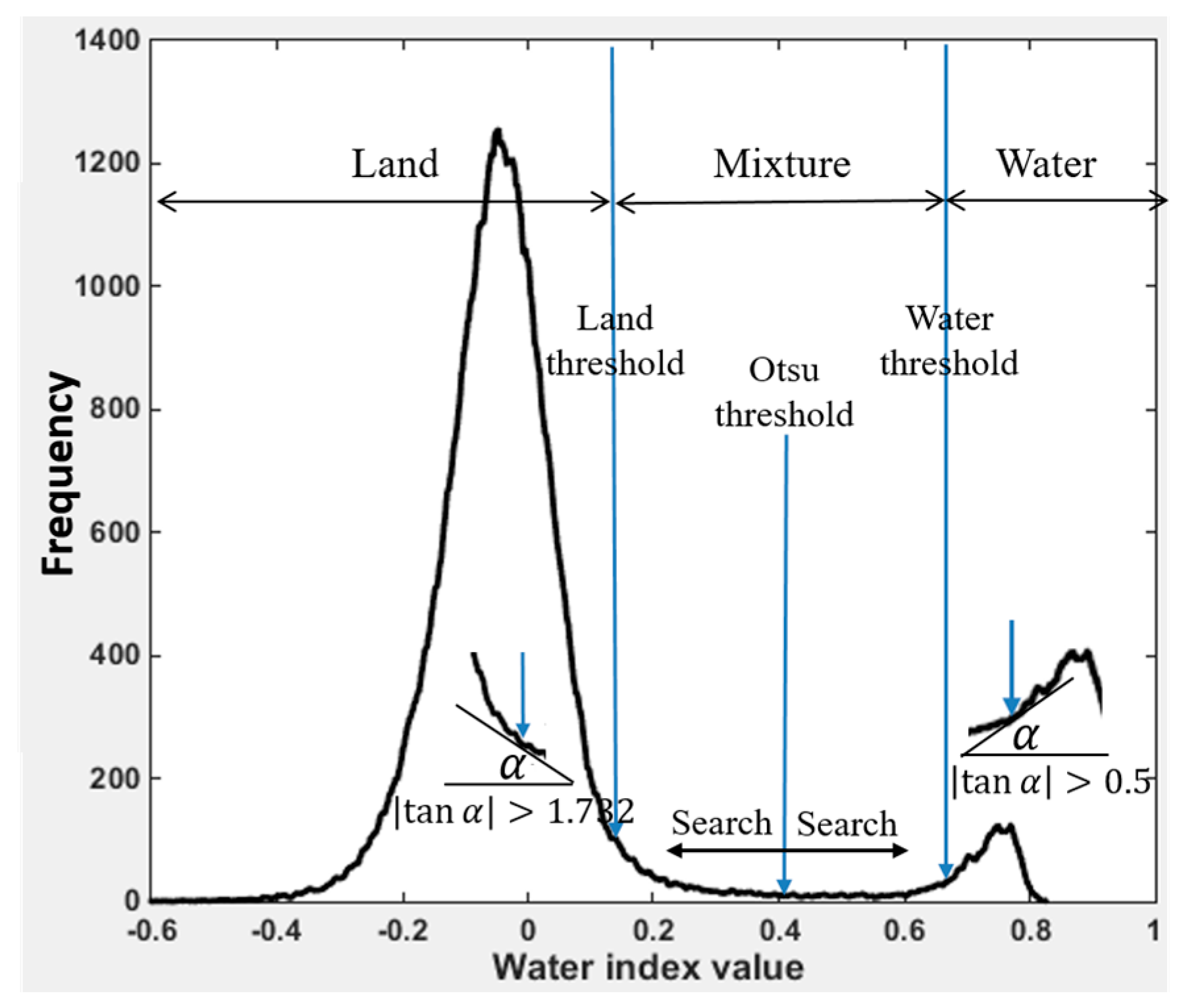
3.1.2. Initial Extraction of Water Pixels and Land Pixels

The Otsu algorithm [32] is utilized for the initial extraction of water pixels and land pixels. The Otsu algorithm is used to select an optimal threshold for the separation by calculating the maximum inter-class variance. The fundamental theorem of the Otsu algorithm can be described as follows: the water index image value is assumed to be within the range [a, …, b], and the water index image can be divided into two parts by a threshold t. The inter-class variance σ² can be calculated as follows:

$${\sigma }^2={\mathrm{w}}_0{\left({\mu }_0-\mu \right)}^2+w_1{\left({\mu }_1-\mu \right)}^2,$$

(2)

$$w_0\cdot {\mu }_0+w_1\cdot {\mu }_1=\mu$$

(3)

where ${\mu }_0$, ${\mu }_1$, and $\mu$ are the mean values of the two parts and the whole of the image. $w_0$ and $w_1$ are the percentage of each part of the image. From Equations (2) and (3), the variance σ² and threshold t can be simply expressed as follows. When σ2 reaches the maximum value, the corresponding t is regarded as the optimal threshold.

$$t=argmax\left[w_0\cdot w_1\cdot {\left({\mu }_1-{\mu }_0\right)}^2\right]$$

(4)

The Ostu method was applied to the histogram of the NDWI image, thereby obtaining the initial water and land pixels.

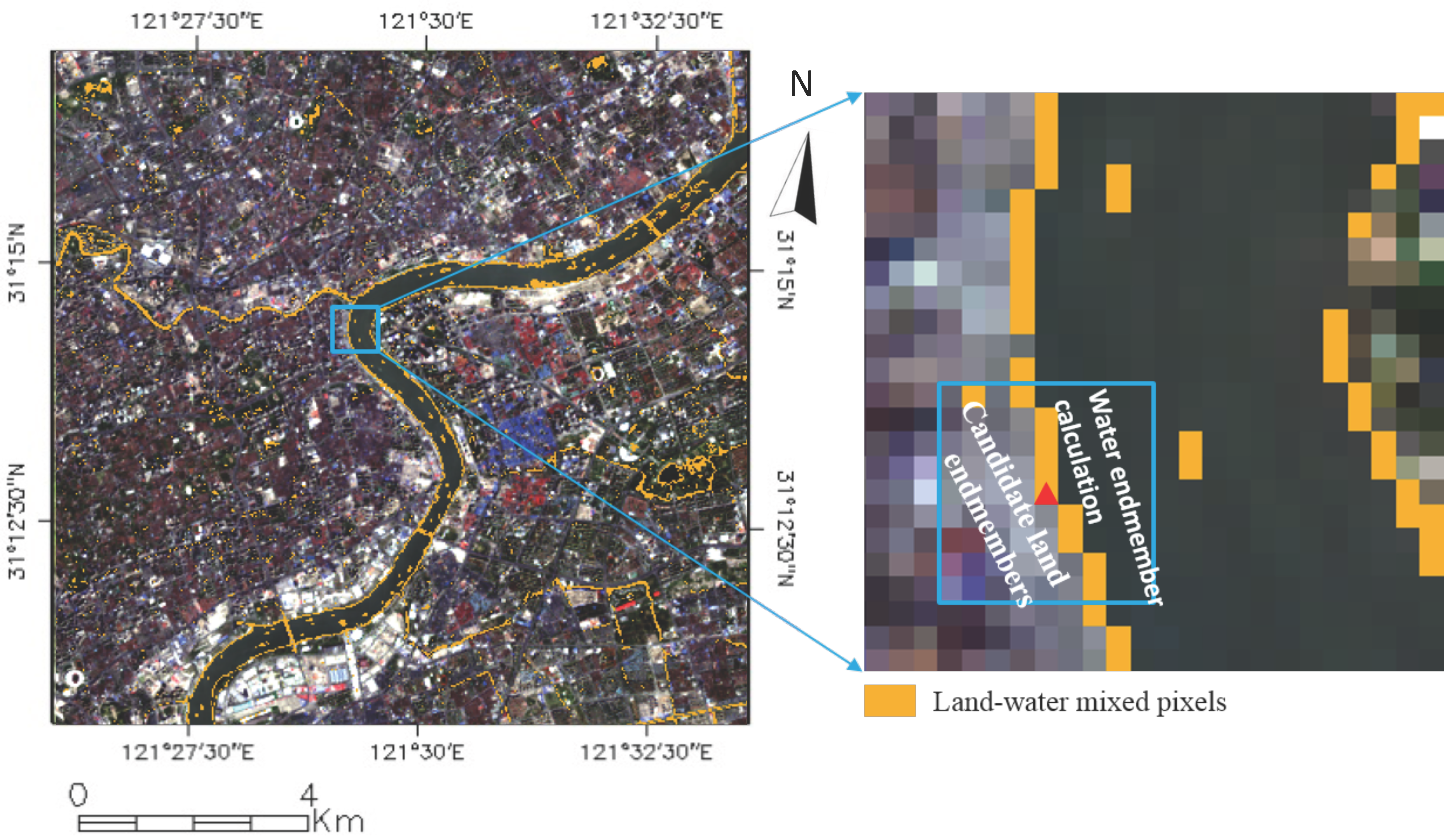
3.1.3. Automated Mixed Land-Water Pixel Extraction

To automatically extract mixed land-water pixels, the Ostu threshold is used as the start value to search for mixed land-water pixels in the NDWI image histogram between the land threshold and the water threshold (see Figure 3). Locally weighted scatter plot smoothing is first applied to the original histogram curve [33]. The slopes of the histogram curve were then used as the discriminant criteria (see Equation (6)). Considering that mixed pixels are much more easily confused with complex land-cover types than pure water pixels, the slopes of the pure land threshold and pure water threshold are set to 60° and 30°, respectively. The corresponding tangential curvatures for pure land and pure water selection can be calculated as follows:

$${\left|\tan \mathsf{\alpha }\right|}_{\text{land},\text{left}}\ge 1.732,{\left|\tan \mathsf{\alpha }\right|}_{\mathrm{water},\mathrm{right}}\ge 0.5$$

(5)

When the curve points of each side first meet the criteria, the corresponding abscissa values are selected as the land and water thresholds.

3.1.4. Misclassification Removal by Simple Post-Processing

Therefore, in this step, two rules are built for misclassification removal as follows:

$${\rho }_{blue}-{\rho }_{green}\le 0,{\rho }_{SWIR1}\le 0.2$$

(6)

where $\rho$ represents the reflectance of the respective bands. The extracted mixed land-water pixels obtained in the previous steps are eliminated if they do not satisfy the above rules. A map of the mixed land-water pixels is then produced (Figure 4).

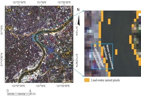
3.2. Endmember Determination by Local Spatial Information

Under the assumption that the endmember signature of a target pixel should be similar to the spatially-adjacent pixels, based on spatial dependence theory, the endmembers of land and water are determined by the neighboring pure land or pure water pixels within a certain distance (see Figure 5). Through experimental comparison, the optimal window size is set to 9 × 9. Based on the previous process described in Section 3.1, the image is divided into three parts: water pixels, land pixels, and mixed land-water pixels. The local window traverses the test image centered at each mixed pixel. The spectrum of the land endmember is then determined by selecting the most representative land pixel by adaptive iteration in the local window, and the spectrum of the water endmember is determined by calculating an average of the water pixels in the local window.

3.3. Linear Unmixing Method

In the linear spectral mixture analysis (LSMA) model, the spectrum of a mixed pixel is assumed to be a linear combination of the endmembers’ spectra weighted by the area coverage of each endmember within the pixel. In this study, the relationship between the reflectivity of a mixed pixel and its endmembers is also considered to be linear. The constraints were imposed that the sum of the endmembers’ abundances should be equal to one and the range of the endmember abundance should be limited to between 0 and 1. The unmixing equations can then be defined as follows:

$${\rho }_m={\rho }_l\times f_l+{\rho }_w\times f_w+\sigma ,$$

(7)

$$f_l+f_w=1,0\le f_l,f_w\le 1$$

(8)

where ${\rho }_l$, ${\rho }_w$, and ${\rho }_m$ are the reflectance values of pure land, pure water, and mixed pixels, respectively. $f_l$ and $f_w$ are the respective abundances of the land and water endmembers, and $\sigma$ is the residual error. According to Equations (7) and (8), the water abundance can be derived as follows:

$$f_w=\frac{{\rho }_m-{\rho }_l-\sigma }{{\rho }_w-{\rho }_l},$$

(9)

subject to:

$${\Vert \sigma \Vert }_1=\min \text{ and min}\le E\left({\Vert \sigma \Vert }_1\right)+3\times \sqrt{D\left({\Vert \sigma \Vert }_1\right)},$$

(10)

In Equation (9), ${\rho }_m$ is the known spectrum of the mixed land-water pixel; ${\rho }_w$ is the average spectrum of the water pixels in the local window; and ${\rho }_l$ is determined by selecting the optimal candidate land pixel in the local window, with the constraint of the minimal L1 norm ${\Vert \sigma \Vert }_1$. Meanwhile, the minimal L1 norm ${\Vert \sigma \Vert }_1$ should meet the requirement of being less than a threshold, which means that the selected optimal endmembers are representative of the true fractions in the mixed pixel. In this study, the threshold is automatically set according to the statistics of the ${\Vert \sigma \Vert }_1$ sets, and $E\left({\Vert \sigma \Vert }_1\right)$ and $\sqrt{D\left({\Vert \sigma \Vert }_1\right)}$ in Equation (10) represent the average value and mean-square error of the ${\Vert \sigma \Vert }_1$ sets, respectively.

3.4. Accuracy Assessment

A quantitative accuracy evaluation is often difficult to implement for the subpixel mapping of surface features because of the difficulty of obtaining a reference map and the lack of quantitative accuracy evaluation indexes. In this study, the water boundaries were extracted from high-precision Google Earth^TM images and applied for the reference water fraction map generation, using a 10 × 10 grids for each pixel for the test images (see Figure 5). As for reducing the impact of the geometric error between the Landsat OLI images and the reference images, a 90 × 90 m² sampling size (3 × 3 pixels size for the OLI image) was adopted for both the reference water maps and the estimated water maps [34,35,36,37].

Spectral unmixing is considered to be a soft classification method, and its output result is the percentage of ground features in each pixel. According to previous research, three types of error measurements are widely used in subpixel classification [34,35,38,39], i.e., RMSE, mean absolute error (MAE), and systematic error (SE). The RMSE and MAE are both used to quantify the relative error of the estimated surface abundance at the pixel level, and the SE indicates the overall trend of the over- or under-estimation. However, all these accuracy evaluation indexes have their limits and cannot comprehensively reflect subpixel classification accuracy. Therefore, the producer’s accuracy, user’s accuracy, and Kappa coefficient expressions were modified to fit with subpixel classification evaluation. The five accuracy measurements can be calculated as follows:

$$Pro.acc={\displaystyle \sum _{\mathrm{i}=1}^{\mathrm{N}}Min\left\{f_i\left(ref\right),f_i\left(esti\right)\right\}}/{\displaystyle \sum _{i=1}^N{f}_i\left(ref\right)}$$

(11)

$$Use.acc={\displaystyle \sum _{i=1}^{M}Min\{f_i\left(ref\right),f_i\left(esti\right)\}}/{\displaystyle \sum _{i=1}^M{f}_i\left(esti\right)}$$

(12)

$$\{\begin{array}{l}Kappa=\left(Po-Pc\right)/\left(1-Pc\right)\\ Pc={\displaystyle \sum _{i=1}^{\text{nm}}{f}_i\left(esti\right)\times {\displaystyle \sum _{i=1}^{nm}{f}_i\left(ref\right)+{\displaystyle \sum _{i=1}^{nm}\left(1-f_i\left(esti\right)\right)\times {\displaystyle \sum _{i=1}^{nm}\left(1-f_i\left(ref\right)\right)}}}}/\left(nm\times nm\right)\\ Po={\displaystyle \sum _{i=1}^{nm}\left(Min\{f_i\left(ref\right),f_i\left(esti\right)\}+1-Max\{f_i\left(ref\right),f_i\left(esti\right)\}\right)}/nm\end{array},$$

(13)

$$RMSE=\sqrt{\frac{1}{n\mathrm{m}}{\displaystyle \sum _{i=1}^{nm}{\left(f_i\left(esti\right)-f_i\left(ref\right)\right)}^2}}$$

(14)

$$SE=\frac{1}{nm}{\displaystyle \sum _{i=1}^{nm}\left(f_i\left(esti\right)-f_i\left(ref\right)\right)}$$

(15)

where Pro.acc and Ues.acc represent the producer’s accuracy and user’s accuracy, respectively. f_i(ref) and f_i(esti) are the water abundance of the pixels of the reference image and estimated image, respectively, and i is the location of each pixel. N and M are the number of mixed land-water pixels in the reference image and estimated image, respectively, and nm is the number of pixels in the whole image.

4. Results

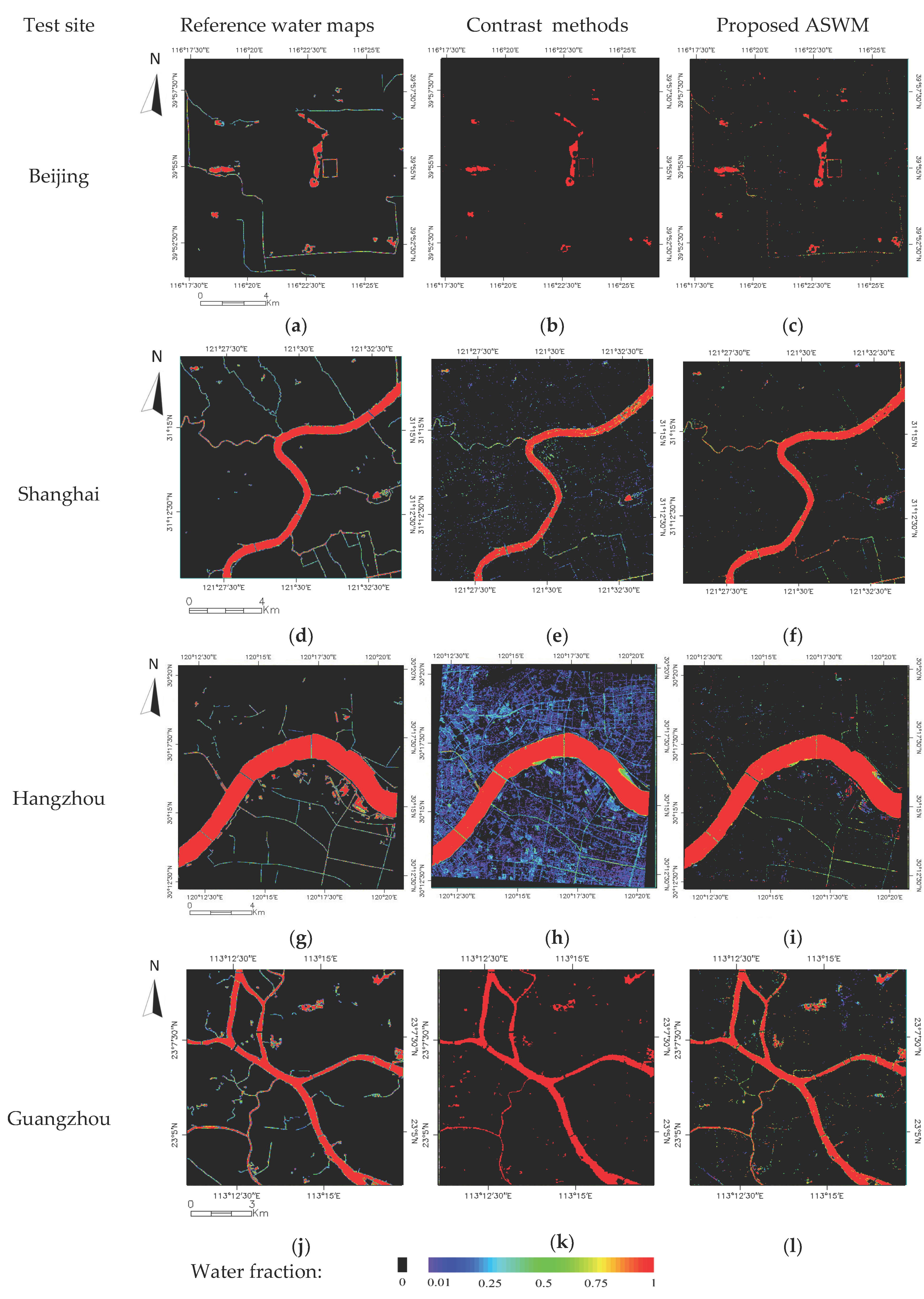
4.1. Water Maps from the Different Methods

To compare the accuracy of ASWM with other methods, both the MNDWI water index method (selecting the optimal water thresholds manually according to the reference image) and a target detection method of constrained energy minimization (CEM) were applied for water extraction at the pixel level [13]. Furthermore, two SMA methods were also adopted for water extraction at the subpixel level in comparison with the proposed method. The first SMA method was the traditional fully-constrained least squares (FCLS) unmixing method [40]. When implementing this method, a pixel purity index (PPI) was first applied to the test images for pure ground feature spectra collection by referencing the high-resolution Google Earth^TM images. The endmember spectra (including vegetation, impervious, soil, and water) were then acquired by averaging the spectra of each ground feature, and finally applied to FCLS for water fraction estimation. The second subpixel method was multiple endmember spectral mixture analysis (MESMA) [41,42]. In this study, with the PPI image computation and Google Earth^TM reference images, four endmember libraries of vegetation, impervious, soil, and water were built. Specifically, as the area of soil in urban areas is not usually large, and the spectral characteristics of soil and impervious surfaces are similar in some cases [34], the spectral libraries of soil and impervious were combined into one endmember library, and the corresponding endmember was called the impervious (soil) endmember. Meanwhile, considering that a considerable amount of shade exists in urban areas, a photometric shade endmember with a uniform reflectance of zero in all bands was introduced to account for the variation in illumination [43]. Then, with the endmember libraries of water, vegetation, impervious (soil), and photometric shade, hundreds of four-endmember models for each test image were built for the MESMA application.

In the first column of Figure 6, the reference maps (Figure 6a,d,g,j) were shown. In the second column of Figure 6, the water maps by the best-performing contrast method are displayed, i.e., the water mapping results of MNDWI for study area 1—Beijing (Figure 6b), MESMA for study area 2—Shanghai (Figure 6e), FCLS for study area 3—Hangzhou (Figure 6h), and CEM for study area 4—Guangzhou (Figure 6k). In the last column of Figure 6, the water mapping results of the ASWM method for the different study areas (Figure 6c,f,i,l) were shown. From a visual inspection, it can be seen that MNDWI and CEM (Figure 6b,k) omit the small water bodies in most cases, while FCLS and MESMA (Figure 6e,h) often misclassify land surface as water. The visual inspection of the surface water maps derived from ASWM suggests that ASWM is able to extract urban water maps with a higher degree of accuracy.

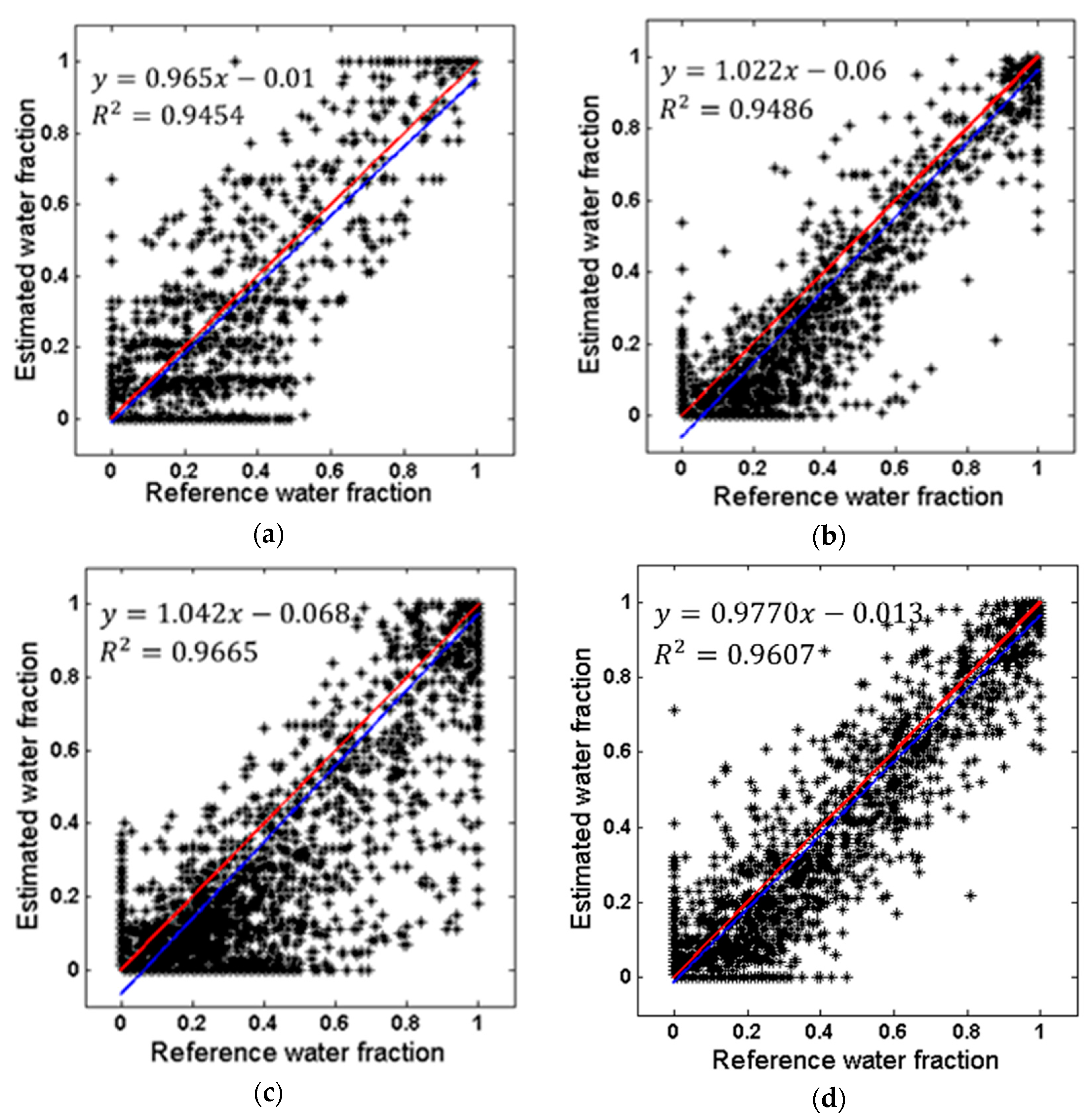
4.2. Accuracy Assessment Results

A scatterplot was first used to examine the correlation between the reference water fractions and the estimated water fractions obtained by the proposed ASWM. As shown in Figure 7, the regression models all have a near 1:1 relationship, supported by their slopes of 0.97, 1.02, 1.04, and 0.98, R-squared values of 0.9454, 0.9486, 0.9665, and 0.9607, and intercepts of −0.01, −0.06, −0.07, and −0.01, for Beijing, Shanghai, Hangzhou, and Guangzhou, respectively.

Five different accuracy assessment approaches (see Section 3.4) are used to compare the water mapping accuracies: user’s accuracy, producer’s accuracy, kappa coefficient, RMSE, and SE. The quantitative subpixel accuracy assessment results are summarized in

Table 2. Summary of the classification accuracy of the four classifiers by study area.

Study Area	Kappa					Producer’s Accuracy
	ASWM	MNDWI	FCLS	MESMA	CEM	ASWM	MNDWI	FCLS	MESMA	CEM
Beijing	0.739	0.610	0.279	0.088	0.211	70.2%	45.8%	87.3%	88.2%	45.22%
Shanghai	0.899	0.842	0.548	0.837	0.442	84.8%	74.3%	88.3%	77.4%	788.0%
Hangzhou	0.900	0.890	0.754	0.855	0.881	88.7%	82.7%	89.1%	49.8%	84.3%
Guangzhou	0.910	0.817	0.729	0.739	0.797	87.5%	71.4%	91.4%	85.9%	79.0%
	User’s accuracy					RMSE
	ASWM	MNDWI	FCLS	MESMA	CEM	ASWM	MNDWI	FCLS	MESMA	CEM
Beijing	79.2%	93.7%	18.4%	0.7%	16.0%	0.046	0.059	0.110	0.209	0.157
Shanghai	97.2%	99.6%	54.8%	93.6%	36.1%	0.045	0.067	0.085	0.058	0.078
Hangzhou	93.3%	99.5%	71.2%	97.5%	94.4%	0.050	0.098	0.110	0.189	0.065
Guangzhou	97.3%	99.2%	64.6%	69.0%	85.9%	0.080	0.085	0.093	0.084	0.151
	SE
	ASWM	MNDWI	FCLS	MESMA	CEM
Beijing	−0.002	−0.011	0.079	0.186	0.039
Shanghai	−0.009	−0.017	0.041	−0.012	0.078
Hangzhou	−0.004	−0.023	0.034	−0.100	−0.010
Guangzhou	−0.014	−0.025	0.037	0.022	−0.011

, where it is clear that the proposed ASWM method significantly outperforms the other four related methods. A close look at the conditional kappa coefficient for each test site reveals that the water maps derived from the proposed method have the highest consistency with the reference water map. The water maps of the four methods are the least accurate in the Beijing test site. For the other test sites, only ASWM has the ability to achieve producer’s accuracy and user’s accuracy values of higher than 84%. The accuracy assessment indicates that ASWM is able to provide an adequate estimation of the surface water fraction, with an average RMSE of 0.055 and an average SE of −0.007. Negative SE values are observed for all the study areas, suggesting that the overall water abundance is under-estimated.

5. Discussion

5.1. Mixed Land-Water Pixel Extraction

This study has explored the extraction of mixed land-water pixels by the use of a water index. Compared to the traditional FCLS and MESMA approaches, the proposed ASWM unmixing algorithm applied only to mixed pixels achieved an improvement both in accuracy and efficiency in the abundance estimation in the experiments.

According to the histogram of the water index image, the mixed land-water pixels always locate between the pure land and pure water thresholds. Therefore, the histogram slopes were used to find these mixed pixels. In order to ensure that the mixed pixels are correctly extracted from the remote sensing images, the pure land and pure water thresholds should locate at the furthest left and right of the bottom of the water index histogram. Accounting for the fact that mixed pixels are mainly confused with land pixels, in the experiments, the thresholds of the slopes of pure water and pure land were set to 30° and 60°, respectively (Figure 3), and the corresponding thresholds of the absolute value of the tangential curvature were 0.5 and 1.732. The following unmixing process also has the effect of removing the wrongly extracted pixels by estimating the water abundances which approach 0 for the wrongly-extracted land pixels, and 100% for the wrongly-extracted water pixels. Several experiments were implemented using images from urban areas of China, and the corresponding kappa coefficient range from 0.8825–0.8994 showed that the final water abundance map result only varied a little when the slope thresholds were set to 30° and 60° for both pure water and pure land extraction, respectively.

In the mixed land-water pixel extraction process, some post-processing is implemented to improve the accuracy of the extraction. In this study, the difference between the green and blue bands was used to eliminate dark building pixels (Equation (6)). This approach works for two main reasons: (1) as a result of eutrophication and human disturbance in urban areas, surface water always contains higher amounts of chlorophyll and suspended sediment. In addition, with the strong spatial dependence between water and vegetation, the vegetation may be the key component of the land-water pixels. Taken together, these factors mean that the green band reflectance of mixed land-water pixels is higher than the blue band [44,45,46]; and (2) most of the land covers that show higher reflectance in the green band than the blue band possess similar characteristics to water bodies; however, dark buildings present opposite characteristics. Above all, the green band and the blue band can be used for separation of mixed land-water pixels and dark buildings. However, it is noticeable that this approach ignores the situation of the mixed land-water pixels being made up of water and dark buildings. Therefore, to retain all of the mixed land-water pixels in the elimination of dark building pixels, although the threshold of Equation (6) was set to zero in this study, the threshold can also be set a little higher than zero to prevent the mixed land-water pixels being removed. In summary, the post-processing aims to remove those land pixels that are clearly distinct from the mixed land-water pixels.

5.2. Endmember Selection

The key to successful SMA is appropriate endmember selection [24,47]. Accounting for spectral variability when selecting endmembers has been pointed out to be an important factor that can severely affect the accuracy of subpixel land-cover fractions [22,35,36,48]. Traditional SMA uses an invariant set of endmembers and it is quite limited when mapping heterogeneous urban surfaces [49,50,51]. MESMA takes the spectral heterogeneity in urban environments into account, and this method divides the image into several classes, where the classes are subdivided into sub-classes as much as possible. The experimental results showed that MESMA achieved better results than the traditional SMA, but consumed more time.

Above all, two issues should be stressed here. Firstly, the endmember spectrum acquisition of the two methods depends on the collection of pure pixels. However, especially for MESMA, it is impossible to obtain all the sub-classes of endmembers through pure pixels in the image. Secondly, to solve the endmember variability problem, researchers need to acquire all of the endmembers of materials in the whole image and consider the compositions by different endmembers of material as much as possible for every pixel; this is hard work for most cases. Actually, in some cases, the “purest” endmembers are not necessarily representative of the fractions within the pixel, and the representative spectra may not necessarily be selected as “pure” endmembers [51]. Therefore, how to select the representative endmembers becomes the most important issue. In ASWM, the whole image is divided into two classes (water and land), and then the most representative endmembers are selected by adaptive iteration in the neighboring pixels. The endmember spectra of water and land are then determined by the adjacent pixels of each mixed pixel. Frankly speaking, this technique for the selection of the most representative endmembers may not be precise enough, and error between the selected land endmember and the true land endmember can exist and can seriously affect the final result. Even so, in this study, the proposed ASWM method still achieved the highest subpixel water extraction accuracy with the lowest RMSE and SE when compared with the other methods.

5.3. Error Analysis

ASWM achieved the highest water mapping accuracy when compared with the other methods; however, errors did exist in the final water maps. In the experiments, the Beijing test area resulted in the lowest water mapping accuracy, with a kappa coefficient of 0.7392, followed by the Shanghai test area, with a kappa coefficient of 0.8994. Through a comprehensive analysis of the error statistics, we believe that the error source comes from three aspects: (1) all four test images were acquired in urban areas with complex ground surface conditions, especially for the Beijing and Shanghai test areas, which include many dark buildings and building shadows, which are easily confused with water bodies due to the high similarity in the spectral features [15]; (2) the technique of the selection of the most representative endmembers, accounting for land surface similarity in an adjacent space, is proposed. However, this may not agree with the spectra of the fractions in the mixed pixels, and could result in large residuals in the unmixing process; and (3) the linear unmixing method was applied for the water abundance estimation in the study; however, the measured signal of the sensor always results from the interactions of electromagnetic radiation with the multiple constituents within each pixel [52]. The multiple scattering between at least two materials in the field of view can make the spectra of a mixed pixel and its fractions not simply linear, so errors will inevitably occur with the application of a linear method.

As stated above, to verify the generalization ability of the new proposed method, four urban areas in the diverse complex urban environments were selected for testing. All of the experiments show the best performance of the proposed method, however, as the proposed method utilized some empirical knowledge for the mixed land-water pixel extraction, further tests are still necessary. Future studies will need to improve the details based on the general processing framework proposed in this study, and the detailed improvements should be able to achieve an even higher accuracy in water extraction.

6. Conclusions

For urban and environmental applications at regional/national scales, urban surface water information should be extracted accurately and not be limited to the pixel level. In this paper, a novel method was presented for urban water mapping with a subpixel precision. In the proposed method, mixed land-water pixels was first exacted from the remote sensing images based on a water index. A linear unmixing method is then applied to each mixed pixel, and the most representative endmembers are selected using the adjacent spatial information. As all the fixed parameters in the process are set in advance, the new ASWM method can also be regarded as a fully automatic approach. Analysis of the results allows a number of conclusions to be made. Firstly, the mixed land-water pixel extraction before unmixing can help to both improve the unmixing accuracy and the computational efficiency. Secondly, with the adjacent spatial similarity, the endmember signatures derived from the adjacent ground surfaces provide a new means of approximating the most representative endmember signatures. Finally, the results of both the water maps and quantitative accuracy assessment indicate that the proposed ASWM method performs reasonably well in the mapping of surface water, with a relatively high subpixel precision.

The future research directions will include reference water map acquisition and accurate registration between reference and test image to better assess the accuracy of the estimated water abundance. In addition, as the confusion between water and other urban materials is an unsolved problem in water extraction, the distinction between surface water and other surface features requires further study. Finally, the method developed in this study has extended the unmixing technique into water mapping in a complex urban environment. Its core idea could also be extended to the extraction of other land covers at the subpixel level. However, there is certainly room for improvement. For instance, the selection of the most representative endmembers by integrating spectral and spatial information, and the consideration of nonlinear factors that influence water abundance estimation should be able to contribute to the achievement of an even higher precision.

References

1. Proud, S.R.; Fensholt, R.; Rasmussen, L.V.; Sandholt, I. Rapid response flood detection using the MSG geostationary satellite. IEEE J. Sel. Top. Appl. Earth Obs. Remote Sens. 2011, 13, 536–544. [Google Scholar] [CrossRef]
2. Feng, L.; Hu, C.M.; Chen, X.L.; Li, R.F.; Tian, L.Q.; Murch, B. MODIS observations of the bottom topography and its inter-annual variability of Poyang Lake. Remote Sens. Environ. 2011, 115, 2729–2741. [Google Scholar] [CrossRef]
3. Prigent, C.; Papa, F.; Aires, F.; Jiménez, C.; Rossow, W.B.; Matthews, E. Changes in land surface water dynamics since the 1990s and relation to population pressure. Geophys. Res. Lett. 2012, 39, 85–93. [Google Scholar] [CrossRef]
4. Güttler, F.N.; Niculescu, S.; Gohin, F. Turbidity retrieval and monitoring of Danube Delta waters using multi-sensor optical remote sensing data: An integrated view from the delta plain lakes to the western–northwestern Black Sea coastal zone. Remote Sens. Environ. 2013, 132, 86–101. [Google Scholar] [CrossRef]
5. Tong, X.; Xie, H.; Qiu, Y.; Zhang, H.; Song, L.; Zhang, Y.; Zhao, J. Quantitative monitoring of inland water using remote sensing: An example of upper reaches of Huangpu River, China. Int. J. Remote Sens. 2010, 31, 2471–2492. [Google Scholar] [CrossRef]
6. Ekercin, S. Coastline change assessment at the Aegean Sea Coasts in Turkey using multitemporal Landsat imagery. J. Coast. Res. 2009, 23, 691–698. [Google Scholar] [CrossRef]
7. Pardo-Pascual, J.E.; Almonacid-Caballer, J.; Ruiz, L.A.; Palomar-Vazquez, J. Automatic extraction of shorelines from Landsat TM and ETM multi-temporal images with subpixel precision. Remote Sens. Environ. 2012, 123, 1–11. [Google Scholar] [CrossRef]
8. Hung, M.C.; Wu, Y.H. Mapping and visualizing the Great Salt Lake landscape dynamics using multi-temporal satellite images, 1972–1996. Int. J. Remote Sens. 2005, 26, 1815–1834. [Google Scholar] [CrossRef]
9. Tulbure, M.G.; Broich, M. Spatiotemporal dynamic of surface water bodies using Landsat time-series data from 1999 to 2011. ISPRS J. Photogramm. 2013, 79, 44–52. [Google Scholar] [CrossRef]
10. Bryant, R.G.; Rainey, M.P. Investigation of flood inundation on playas within the Zone of Chotts, using a time-series of AVHRR. Remote Sens. Environ. 2002, 82, 360–375. [Google Scholar] [CrossRef]
11. Jain, S.K.; Singh, R.D.; Jain, M.K.; Lohani, A.K. Delineation of flood-prone areas using remote sensing technique. Water Resour. Manag. 2005, 19, 337–347. [Google Scholar] [CrossRef]
12. McFeeters, S.K. The use of normalized difference water index (NDWI) in the delineation of open water features. Int. J. Remote Sens. 1996, 17, 1425–1432. [Google Scholar] [CrossRef]
13. Xu, H. Modification of normalised difference water index (NDWI) to enhance open water features in remotely sensed imagery. Int. J. Remote Sens. 2006, 27, 3025–3033. [Google Scholar] [CrossRef]
14. Feyisa, G.L.; Meilby, H.; Fensholt, R.; Proud, S.R. Automated Water Extraction Index: A new technique for surface water mapping using Landsat imagery. Remote Sens. Environ. 2014, 140, 23–35. [Google Scholar] [CrossRef]
15. Xie, H.; Luo, X.; Xu, X.; Tong, X.; Jin, Y.; Pan, H.; Tong, X. New hyperspectral difference water index for the extraction of urban water bodies by the use of airborne hyperspectral images. J. Appl. Remote Sen. 2014, 8, 5230–5237. [Google Scholar] [CrossRef]
16. Yang, Y.; Liu, Y.; Zhou, M.; Zhang, S.; Zhan, W.; Sun, C.; Duan, Y. Landsat 8 OLI image based terrestrial water extraction from heterogeneous backgrounds using a reflectance homogenization approach. Remote Sens. Environ. 2015, 171, 14–32. [Google Scholar] [CrossRef]
17. Ghrefat, H.A.; Goodell, P.C. Land cover mapping at Alkali Flat and Lake Lucero, White Sands, New Mexico, USA using multi-temporal and multi-spectral remote sensing data. Int. J. Appl. Earth Obs. 2011, 13, 616–625. [Google Scholar] [CrossRef]
18. Guo, Y.L.; Li, Y.M.; Zhu, L.; Liu, G.; Wang, S.; Du, C.G. An Improved Unmixing-Based Fusion Method: Potential application to remote monitoring of inland waters. Remote Sens. 2015, 7, 1640–1666. [Google Scholar] [CrossRef]
19. Hommersom, A.; Wernand, M.R.; Peters, S.; Eleveld, M.A.; van der Woerd, H.J.; de Boer, J. Spectra of a shallow sea-unmixing for class identification and monitoring of coastal waters. Ocean. Dyn. 2011, 61, 463–480. [Google Scholar] [CrossRef]
20. Wang, Q.; Atkinson, P.M.; Shi, W. Fast subpixel mapping algorithms for subpixel resolution change detection. IEEE Trans. Geosci. Remote Sens. 2015, 53, 1692–1706. [Google Scholar] [CrossRef]
21. Wang, Q.; Shi, W.; Atkinson, P.M.; Li, Z. Land cover change detection at subpixel resolution with a Hopfield neural network. IEEE J. Sel. Top. Appl. Earth Obs. Remote Sens. 2015, 8, 1339–1352. [Google Scholar] [CrossRef]
22. Shi, C.; Wang, L. Incorporating spatial information in spectral unmixing: A review. Remote Sens. Environ. 2014, 149, 70–87. [Google Scholar] [CrossRef]
23. Li, H.; Zhang, L. A hybrid automatic endmember extraction algorithm based on a local window. IEEE Trans. Geosci. Remote Sens. 2011, 49, 4223–4238. [Google Scholar] [CrossRef]
24. Somers, B.; Asner, G.P.; Tits, L.; Coppin, P. Endmember variability in Spectral Mixture Analysis: A review. Remote Sens. Environ. 2011, 115, 1603–1616. [Google Scholar] [CrossRef]
25. Zare, A.; Gader, P.; Bchir, O.; Frigui, H. Piecewise convex multiple-model endmember detection and spectral unmixing. IEEE Trans. Geosci. Remote Sens. 2013, 51, 2853–2862. [Google Scholar] [CrossRef]
26. Sun, D.; Yu, Y.; Goldberg, M.D. Deriving water fraction and flood maps from MODIS images using a decision tree approach. IEEE J. Sel. Top. Appl. Earth Obs. Remote Sens. 2011, 4, 814–825. [Google Scholar] [CrossRef]
27. Ma, B.; Wu, L.; Zhang, X.; Li, X.; Liu, Y.; Wang, S. Locally adaptive unmixing method for lake-water area extraction based on MODIS 250 m bands. IEEE J. Sel. Top. Appl. Earth Obs. Remote Sens. 2014, 33, 109–118. [Google Scholar]
28. Sethre, P.R.; Rundquist, B.C.; Todhunter, P.E. Remote detection of Prairie Pothole Ponds in the Devils Lake Basin, North Dakota. GISci. Remote Sens. 2005, 42, 277–296. [Google Scholar] [CrossRef]
29. Applied Analysis Inc. Subpixel Classifier for IMAGINE: User’s Guide; Applied Analysis Inc.: Billerica, MA, USA, 1997. [Google Scholar]
30. Ji, L.; Zhang, L.; Wylie, B. Analysis of dynamic thresholds for the normalized difference water index. Photogramm. Eng. Remote Sens. 2009, 75, 1307–1317. [Google Scholar] [CrossRef]
31. Xie, H.; Luo, X.; Xu, X.; Pan, H.; Tong, X. Evaluation of Landsat 8 OLI imagery for unsupervised inland water extraction. Int. J. Remote Sens. 2016, 37, 1826–1844. [Google Scholar] [CrossRef]
32. Otsu, N. A threshold selection method from gray-level histograms. IEEE Trans. Syst. Man Cybern. 1979, 9, 62–66. [Google Scholar]
33. Cleveland, W.S. Robust locally weighted regression and smoothing scatterplots. J. Am. Stat. Assoc. 1979, 74, 829–836. [Google Scholar] [CrossRef]
34. Deng, C.; Wu, C. A spatially adaptive spectral mixture analysis for mapping subpixel urban impervious surface distribution. Remote Sens. Environ. 2013, 133, 62–70. [Google Scholar] [CrossRef]
35. Powell, R.L.; Roberts, D.A.; Dennison, P.E.; Hess, L.L. Sub-pixel mapping of urban land cover using multiple endmember spectral mixture analysis: Manaus, Brazil. Remote Sens. Environ. 2007, 106, 253–267. [Google Scholar] [CrossRef]
36. Roberts, D.A.; Quattrochi, D.A.; Hulley, G.C.; Hook, S.J.; Green, R.O. Synergies between VSWIR and TIR data for the urban environment: An evaluation of the potential for the Hyperspectral Infrared Imager (HyspIRI) Decadal Survey mission. Remote Sens. Environ. 2012, 117, 83–101. [Google Scholar] [CrossRef]
37. Wu, C. Normalized spectral mixture analysis for monitoring urban composition using ETM+ imagery. Remote Sens. Environ. 2004, 93, 480–492. [Google Scholar] [CrossRef]
38. Hu, X.; Weng, Q. Estimating impervious surfaces from medium spatial resolution imagery using the self-organizing map and multi-layer perceptron neural networks. Remote Sens. Environ. 2009, 113, 2089–2102. [Google Scholar] [CrossRef]
39. Wu, C.; Murray, A.T. Estimating impervious surface distribution by spectral mixture analysis. Remote Sens. Environ. 2003, 84, 493–505. [Google Scholar] [CrossRef]
40. Heinz, D.C.; Chang, C.I. Fully constrained least squares linear spectral mixture analysis method for material quantification in hyperspectral imagery. IEEE Trans. Geosci. Remote Sens. 2001, 39, 529–545. [Google Scholar] [CrossRef]
41. Roberts, D.A.; Gardner, M.; Church, R.; Ustin, S.; Scheer, G.; Green, R.O. Mapping Chaparral in the Santa Monica Mountains using multiple endmember spectral mixture models. Remote Sens. Environ. 1998, 65, 267–279. [Google Scholar] [CrossRef]
42. Franke, J.; Roberts, D.A.; Halligan, K.; Menz, G. Hierarchical Multiple Endmember Spectral Mixture Analysis (MESMA) of hyperspectral imagery for urban environments. Remote Sens. Environ. 2009, 113, 1712–1723. [Google Scholar] [CrossRef]
43. Dennison, P.E.; Roberts, D.A. Endmember selection for multiple endmember spectral mixture analysis using endmember average RMSE. Remote Sens. Environ. 2003, 87, 123–135. [Google Scholar] [CrossRef]
44. Gitelson, A.A.; Gao, B.C.; Li, R.R.; Berdnikov, S.; Saprygin, V. Estimation of chlorophyll-a concentration in productive turbid waters using a Hyperspectral Imager for the Coastal Ocean—The Azov Sea case study. Environ. Res. Lett. 2011, 6, 024023. [Google Scholar] [CrossRef]
45. Song, K.; Li, L.; Tedesco, L.P.; Li, S.; Duan, H.; Liu, D.; Zhao, Y. Remote estimation of chlorophyll-a in turbid inland waters: Three-band model versus GA-PLS model. Remote Sens. Environ. 2013, 136, 342–357. [Google Scholar] [CrossRef]
46. Mueller, N.; Lewis, A.; Roberts, D.; Ring, S.; Melrose, R.; Sixsmith, J.; Ip, A. Water observations from space: Mapping surface water from 25 years of Landsat imagery across Australia. Remote Sens. Environ. 2016, 174, 341–352. [Google Scholar] [CrossRef]
47. Elmore, A.J.; Mustard, J.F.; Manning, S.J.; Lobell, D.B. Quantifying vegetation change in semiarid environments: Precision and accuracy of spectral mixture analysis and the normalized difference vegetation index. Remote Sens. Environ. 2000, 73, 87–102. [Google Scholar] [CrossRef]
48. Weng, Q. Remote sensing of impervious surfaces in the urban areas: Requirements, methods, and trends. Remote Sens. Environ. 2012, 117, 34–49. [Google Scholar] [CrossRef]
49. Liu, T.; Yang, X. Mapping vegetation in an urban area with stratified classification and multiple endmember spectral mixture analysis. Remote Sens. Environ. 2013, 133, 251–264. [Google Scholar] [CrossRef]
50. Lu, D.; Weng, Q. Spectral mixture analysis of the urban landscape in indianapolis with Landsat ETM+ imagery. Photogramm. Eng. Remote Sens. 2004, 70, 1053–1062. [Google Scholar] [CrossRef]
51. Song, C. Spectral mixture analysis for subpixel vegetation fractions in the urban environment: How to incorporate endmember variability? Remote Sens. Environ. 2005, 95, 248–263. [Google Scholar] [CrossRef]
52. Keshava, N.; Mustard, J.F. Spectral unmixing. Proc. IEEE 2002, 19, 44–57. [Google Scholar] [CrossRef]
Figure 1. Study areas: Beijing, Shanghai, Hangzhou, and Guangzhou, China, illustrated in false-color composite (RGB: bands 6, 5, 2) Landsat OLI images overlaid by the main water bodies of these areas.
Remotesensing 08 00584 g001
Figure 2. Flowchart of the proposed ASWM method.
Remotesensing 08 00584 g002
Figure 3. Histogram of the NDWI at the Shanghai test site.
Remotesensing 08 00584 g003
Figure 4. Maps showing the processing of the mixed land-water pixel extraction. (a) Landsat OLI true-color composite (RGB: bands 4, 3, 2) image of the Shanghai test site; (b) true water boundaries acquired from the high spatial resolution Google EarthTM images; and (c) mixed land-water pixels derived from the water index.
Remotesensing 08 00584 g004
Figure 5. Endmember determination based on adjacent pixels (Landsat OLI true-color composite (RGB: bands 4, 3, 2)).
Remotesensing 08 00584 g005
Figure 6. Comparison of the water mapping results. First row: reference map, water map from the contrast method of MNDWI, and result of the proposed method of Beijing corresponding to (ac); Second row, reference map, water map from the contrast method of MESMA, and result of the proposed method of Shanghai corresponding to (df); Third row, reference map, water map from the contrast method of FCLS, and result of the proposed method of Hangzhou corresponding to (gi); Fourth row, reference map, water map from the contrast method of CEM, and result of the proposed method of Guangzhou corresponding to (jl).
Remotesensing 08 00584 g006
Figure 7. Comparison between the reference and estimated water fractions obtained by ASWM, where the red line is the 1:1 reference line, and the blue line is the regression line. (ad) represent the results for the study areas of Beijing, Shanghai, Hangzhou, and Guangzhou, respectively.
Remotesensing 08 00584 g007