1. Introduction
The ocean wave is one of the most common ocean undulation phenomena and is critically important for ocean research and ocean exploitation [
1,
2,
3,
4,
5,
6,
7]. Many offshore operations like the tensioning of a tanker, cargo transfer, and helicopter landing demand a deterministic prediction of the sea surface field in real-time [
8,
9,
10,
11,
12,
13,
14,
15]. In [
13], the accurate real-time prediction of the sea surface field at the position of an operation platform is completely dependent on the retrieved sea wave components from a measured area in the vicinity of the platform [
9,
10,
11,
12,
13,
14,
15,
16]. In our paper, the wave component denotes the individual sine or cosine waves, since the sea surface can be seen as the superposition of numerous sine or cosine wave. The extracted sea wave components could be directly used as an input to initialize a wave propagation model, and then, to predict a real-time platform motion [
13,
14]. In addition, the sea wave components provide a low-cost approach to investigating the spatial and temporal development of 3D ocean surface fields [
15] and the properties of individual wave components [
17]. Hence, the accuracy of the retrieved sea wave components is one of the most important aspects in the real-time prediction of the sea surface field.
Thus far, most research on retrieving the sea wave components focuses on X-band marine radar for its economy and popularity, and the linear wave model because of its computational efficiency [
9,
10,
11,
13,
14,
15,
16]. The X-band marine radar is commonly used to monitor moving vessels and to derive the statistical sea state parameters such as significant wave height, peak period, wave direction, bathymetry and ocean surface currents from coastal areas or moving platforms [
17,
18,
19,
20,
21,
22,
23,
24,
25]. Now, with recent advances in computer technologies and marine radar techniques, it has the ability to retrieve the sea wave components from an X-band marine radar image sequence [
16,
19].
The method of retrieving the sea wave components, which can be fed into the wave propagation model, was first proposed in [
11,
12]. The 1D time series of the wave components were derived from the retrieved sea surface field. In [
16,
19], by using a 3D discrete Fourier transform (DFT) on the acquired X-band marine radar image sequence, a passband filter was used to select wave-related components in a wavenumber frequency domain. Since the X-band marine radar image is mainly modulated by hydrodynamic modulation, tilt modulation and shadowing, the sea clutter radar image intensities do not stand for the ocean surface field [
1,
2,
3,
4,
5,
6,
7,
9,
15]. An empirical modulation transfer function (MTF) is needed to calibrate the amplitude spectrum [
21,
22,
23,
24,
25]. Subsequently, an inverse 3D DFT method was used to reconstruct the sea surface field, which was used to retrieve the significant wave height. The sea surface field can also be obtained by summing all the individual wave components selected from the passband filter [
11,
12]. Compared with the method of summing all the individual wave components, the inverse 3D DFT method has the advantage of high accuracy and reconstructs the sea surface field quickly. In [
3,
17], the empirical methods to retrieve the ocean surface field in spatial and temporal domains were proposed. The radar image sequence was also decomposed into a wavenumber frequency domain with the 3D DFT method. In [
3,
17], the tilt modulation was considered as a major effect on retrieving the sea surface field. In [
16,
19], shadowing that has a significant influence on the radar image was taken into account at grazing incidence.
The individual wave components could be directly determined by the wave amplitude spectra after the filtering process and applying the modulation transfer function on the amplitude and phase spectra in [
3,
16,
17,
19]. In order to provide an effective prediction, the input requirement of the wave propagation model is that the frequency and wavenumber of the wave components should exactly match the dispersion relation. However, neither the 1D time series of wave components, which is retrieved from the sea surface field, nor the individual wave components, which can be directly retrieved from the frequency wavenumber spectrum after a 3D DFT on the radar image sequence, follow the requirement. Since the 3D DFT was taken on the radar image sequence in the spatial and temporal domain, the uniform frequency and the uniform wavenumber do not strictly satisfy the dispersion relation because of the limited analysis area selected from the image sequence, even though perfect linear synthetic wave data was used [
13,
14]. In addition, the spectral leakage existed in both the spatial and temporal domains, since the analysis area selected was finite [
13,
26], which may become a problem for estimating the wave surface field in the position of a platform. Furthermore, the empirical MTF requires an external equipment as the reference which increases the expense. Using the fixed MTF to different amplitude spectrum may also produce errors for retrieving wave components. Therefore, the resulting errors were introduced into the retrieved wave components, which could deteriorate the prediction of the wave surface field and the motion estimation of the offshore platform.
In order to make the retrieved wave components strictly satisfy the dispersion relation, various filtering methods have been put forward to manipulate the wavenumber and the frequency of the spectrum after taking the 3D DFT on the radar image sequence [
13,
16]. Nevertheless, the accuracy of the reconstructed wave field and the retrieved wave components were not optimal, since a bandpass filter was used and the extracted wave components were susceptible to the bandpass filter. To satisfy the requirement of the wave propagation model, a 2D DFT is applied to retrieve the directional wave components in [
27]. The synthetic radar images, which were synthesized with linear waves while taking tilt modulation and shadowing, were used to verify its effectiveness. For this method, the significant wave height should be considered as prior information. In [
10], a dynamic averaging and evolution scenario that integrates the inversion of the acquired radar images was used to provide a sea surface field prediction. A 4D Var assimilation method was proposed to predict the sea surface field in [
28]. In [
15], based on a multi-directional sea wave model, a method using the 2D DFT on the acquired radar image to predict the sea surface field at a desired location and time was proposed.
Our primary goal in this paper is to propose a new successive cancellation algorithm, which is an alternative to the 3D DFT method and fully based on theory, to efficiently and effectively extract the individual wave components without any reference measurements, whose frequency and wavenumber rigorously satisfy the linear dispersion relation and which can be directly used to initialize the wave propagation model.
This paper is organized as follows:
Section 2 presents the linear dispersion relation and the sea wave model. The detailed derivation and the successive cancellation algorithm to recover the wave components based on the sea wave model are given in
Section 3. In
Section 4, the validity of the proposed method is investigated by computer simulation. Finally, the conclusion is summarized in
Section 5.
Notation: Scalars, vectors and matrices are expressed by regular, bold lowercase letters and bold uppercase letters, respectively. stands for the element of a matrix, . The superscript , and indicate the Hermitian transpose, transpose and complex conjugate, respectively. denotes the DFT operator of the expression in brackets. stands for the Frobenius norm (F-norm or norm-two). represents the real part of a complex number. denotes the complex domain. is a scalar and is a matrix.
2. Sea Wave Model
In this section, we briefly review the concepts of the linear wave theory and the sea wave model.
It is known that under the assumption of the linear wave theory, oceanic surface gravity waves are dispersive with the dispersion relation, given by [
1,
21,
22]
where
w is an angular frequency,
k represents the modulus of wavenumber,
g is the gravity acceleration and
h denotes a water depth. For gravity waves in infinitely deep water, Equation (1) can be simplified as
The ocean surface waves can be seen as the superposition of a number of wave components with different frequencies, amplitudes, wave directions and phases. Based on a linear wave model [
15,
16,
25], a wave field,
, at spatial coordinates
x,
y, and a temporal coordinate
t is given by
where
N is the frequency number,
M is the number of wave component directions,
stands for a discrete amplitude,
is a directional wave spectrum,
denotes a wave frequency,
is a wave component direction,
is the modulus of wavenumber and
is a uniformly distributed initial phase on an interval
. Since the wave images are composed of discrete data, we divide the wave frequency and wavenumber into
parts. The wave angular frequency can be written as
where
is angular frequency resolution. For presentation clarity, Equation (3) can be recasted as
where
and
3. Retrieving the Individual Wave Components
The sea surface field consists of a linear superposition of several individual wave components. If we can obtain each linear wave component whose angular frequency and wavenumber strictly match the dispersion relation, then the retrieved linear wave components can be directly utilized as an input to initialize the wave propagation model, and then to predict the sea surface field at the position of an operation platform and estimate a platform motion. Meanwhile, the sea surface field, which has free selection of temporal and spatial resolution, can be reconstructed by summing all the individual wave components. Our main purpose in this section is to propose a novel method to attain all the wave components by using the sea wave model.
3.1. 1D DFT on the Radar Image Sequence
When the spatial analysis area of a radar image is selected, the sea surface field can be sampled and written as a 2D matrix
for time
t. Suppose that
M and
N represent the sampling numbers in the
x and
y directions of the radar image, respectively. Then, the wave field can be represented as
, where
and
. Thus, Equation (5) can be represented in a more compact matrix form as
where
, the
elements of
and
are
and
, respectively. Now, we discretize the time
t with a sample interval
, which coincides with the radar rotation time. The frequency resolution can be represented as
and then, the radar image sequence
is achieved, where
and
. After that, we take DFT at each location of the sea surface field so that
from which an
M by
N Fourier coefficient matrix
can be attained. In this case, the sea surface field is expressed as Fourier series.
3.2. Fourier Coefficient Matrix Decomposition
Just as we have seen from Equation (
6), by taking the 1D DFT on the radar image sequence
, we obtain
. The
element of
can be explicitly rewritten as
where
, which contains the amplitude and the phase information, are called modulated parameters in this paper. Based on the expression of Equation (7), it would be important to notice that the Fourier coefficient matrix
can be decomposed into two matrices terms
and
and each term can be subsequently decomposed as the product of matrices, which is represented as
where
and
.
is the modulated parameters matrix that is equal to
,
and
. Vector
and
are given by
and
, respectively. Therefore, the sea surface elevation with frequency
denoted by Equation (8) can be rewritten as
Here, it is observed clearly that each term of Equation (9) only involves one wave component direction , which corresponds to two terms and . For the fixed frequency , the sea surface elevation and the wavenumber are given. Thus, Equation (9) is a function of modulated parameters and and wave component direction . Suppose that the two terms containing are moved to the left side of Equation (9) and then the right side is the terms involving , and . For the left side, we take an F-norm on it, and, then, by solving a optimization problem, we take the derivative with respect to modulated parameters and . Thus, a relation between modulated parameters and direction can be achieved. Subsequently, substituting the relation into F-norm expression, it becomes a function that only involves . In the previous section, we have discretized the wave component direction into the M direction. Therefore, we can find a direction that minimizes the F-norm of expression by searching the M discrete component directions. After that, the value of modulated parameters and can be obtained through the above achieved relation and the chose direction , and, then, the amplitude and the phase of the sea wave component are determined.
Up to now, the left side is known to us. Then, we continue to shift the terms containing direction
to the left side. Similarly, all the directions, amplitudes and initial phases of the wave components can be achieved by repeating the above process. The detailed derivation and analysis of the successive cancellation algorithm are given in
Appendix A. The complete successive cancellation algorithm for extracting all the wave components is now depicted below.
3.3. Successive Cancellation Algorithm
By investigating the data structure uncovered by the matrix decomposition in Equation (9) and the above analysis, it motivates us to propose the following successive cancellation algorithm, which first optimizes the direction parameters
by iteratively moving the terms containing the direction parameters
and then estimates the corresponding modulated parameters
.
Given
, initially retrieve modulated parameters
and direction parameter
by solving the following optimization problem:
where
(more detail is in
Appendix A).
Suppose that all previous extractions of
and
for
are completely correct. Now, successively retrieve the modulated parameters
and direction parameter
by solving the following optimization problem:
for
, where
In addition, the solution in Equation (10) can be efficiently obtained by the following two steps:
- (a)
The direction parameters
are extracted by solving the optimization problem below:
- (b)
The modulated parameters and are determined by
Thus, the parameters of amplitude , initial phase and direction of the individual wave components of the sea wave model can be obtained by the above successive cancellation algorithm. In the algorithm, for each index m, it traverses all the M wave component directions to search for the suitable discrete direction value , and then it iterates M times to attain all the wave component directions. Hence, the overall complexity of the algorithm is .
4. Results and Analysis of Experiment
In this section, we carry out radar image simulations at different sea state conditions to examine the validity of our proposed method for retrieving the individual wave components. In order to simplify the problem, the perfect linear synthetic wave data is used. The performance of our method recovering the amplitude and the phase parameters of the individual wave components is presented. The sea surface field is reconstructed by summing all the retrieved wave components achieved. Moreover, the performance of the 3D DFT method retrieving the sea wave components and the sea surface field reconstructed by using the 3D inverse DFT method are presented as a reference. The reconstruction accuracy of the sea surface field of our successive cancellation algorithm is shown by comparing with that of the other method. The experiment and analysis results are shown as follows.
4.1. Radar Image Sequence Simulated with Single Wave
For the primary test, the radar image sequence is simulated with a monochromatic wave. The wave parameters with the significant wave height m, wave length m ( rad/m), wave direction , wave period s ( rad/s) and initial phase are used. In this study, a 3D image sequence is simulated. The spatial resolution of the image is m. For the time domain of the wave image sequence, the time resolution is s. After 1D DFT on the radar image sequence at each position, the Fourier coefficient matrix is the input of our novel iterative algorithm. Based on our method, all the parameters of the wave component including the component direction, the amplitude, initial phase, the wave angular frequency and the wavenumber can be almost exactly recovered. However, it should mentioned that, in our experiment, there is a 180 degree direction ambiguity, since the minimized always corresponds to two different wave directions. The reason might be that the F-norm used in our method possibly causes this ambiguity. In practice, the dominant wave direction can be easily known beforehand, and the directions of most wave components are close to it. Thus, we can choose the one that is relatively close to the dominant wave direction. It is validated that the novel successive cancellation algorithm has the capability to estimate the single wave component from the radar image sequence.
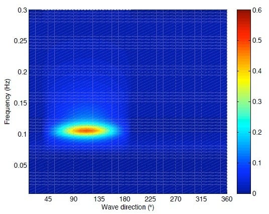
4.2. The Simulation of Radar Image Sequence with Random Wave Field
Real waves in nature are always random and irregular. Our acquired radar image sequence which does not satisfy the input requirement has only 32 continuous images. Hence, we have to use the simulated radar image sequence to certify the effectiveness of our method. The simulation of the sea field is commonly based on the Joint North Sea Wave Project (JoNSWaP) spectrum
[
16,
25]. Since
is in 1D form and the multi-directional characteristic of ocean waves, a Mitsuyasu-type directional spreading function
is used:
where
is the directional wave spectrum,
is the dominant wave direction, and Γ is the gamma function. The parameter
s leads to the angular distribution and varies with the frequency. The wave conditions are initialized with the significant wave height
m, the dominant wave direction
and the peak wave period
s. The angular frequency and the direction of the wave components are uniformly discretized with
rad/s and
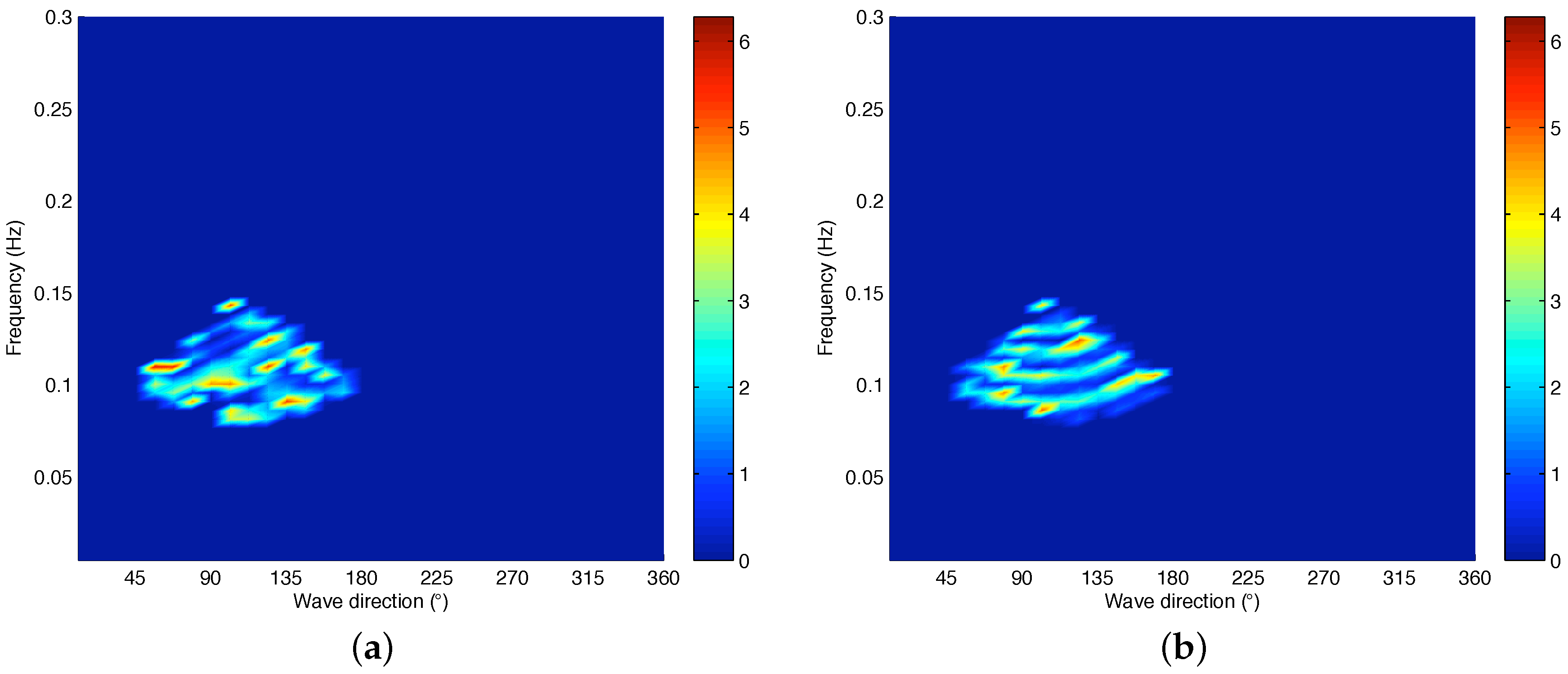
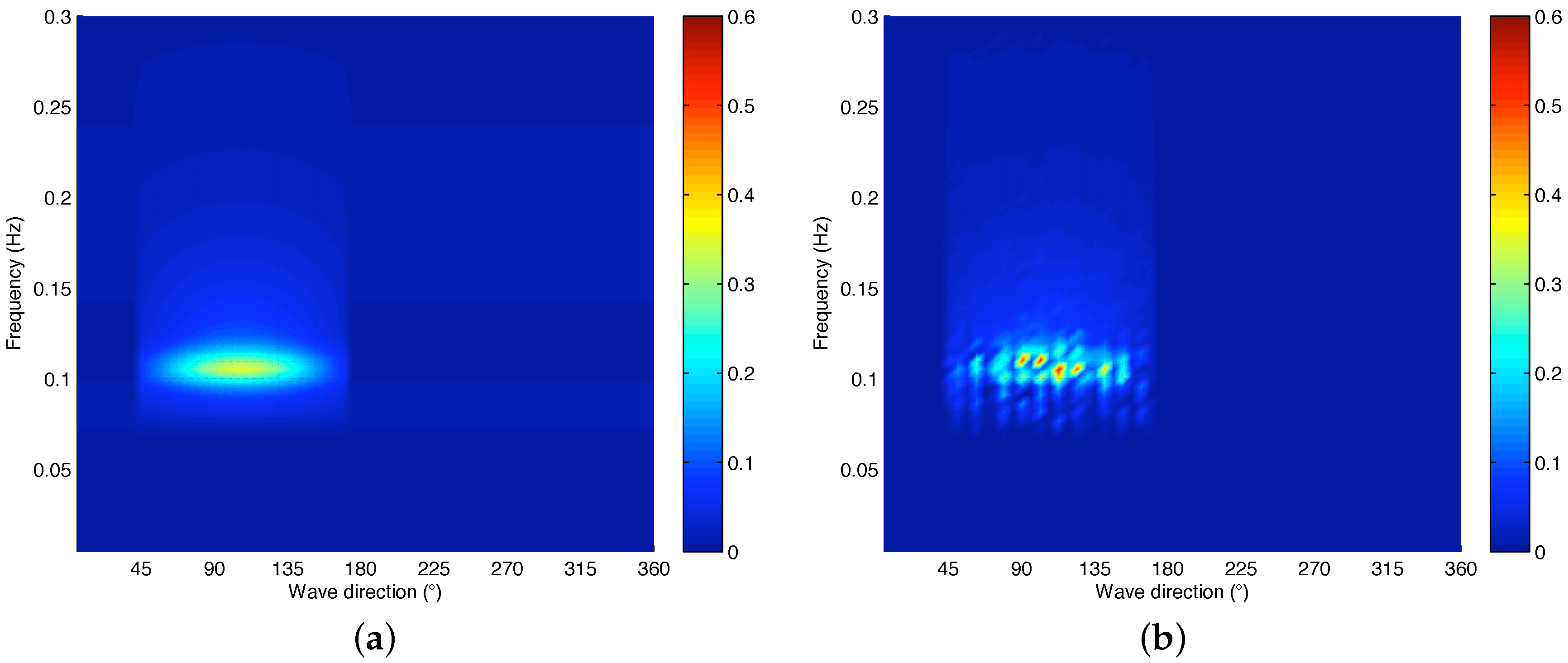
, respectively. Then, the simulated amplitude of the wave components can be obtained by the directional wave spectrum, which is shown in
Figure 1a. The temporal resolution of the wave image sequence is about
s. The image sequence contains 127 continuous images, where
. This means that about 4000 individual wave components are considered. Thus, the 3D
radar image sequence is generated by summing all the linear wave components as Equation (3). The spatial resolution is
m. The hydrodynamic and tilt modulation have a minor impact on the imaging mechanism at grazing incidence, while the shadowing modulation plays an important role [
16,
19]. Hence, we only take shadowing into account in our simulation. Here, we assume that an antenna is 20 m above the mean sea level and the location of the selected region from the radar platform is 300 m. Since the shadowing mask is time variant and the real radar image is non-stationary, it is unreasonable to retrieve parameters by taking 1D DFT on the image sequence without any calibration in subsequent processing. Here, we use ten fixed shadowing masks to produce ten radar image sequences based on the simulated sea surface field sequence, and then we average the retrieved parameters from the ten radar image sequences in our simulation. In our future research, we will develop a time frequency analysis method to directly retrieve parameters from the marine radar image sequence. The simulated radar image is shown in
Figure 1b at
s.
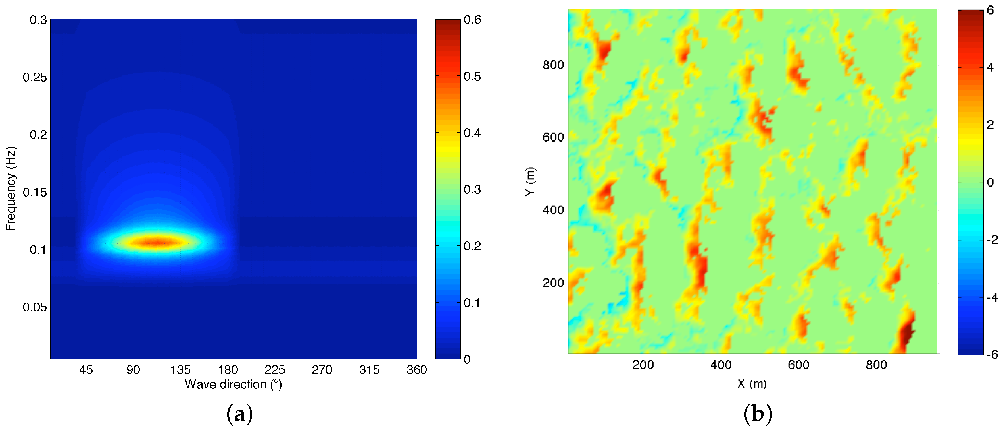
The 3D DFT method and our method are both used to retrieve the amplitude and the phase from the radar image sequence.
Figure 2 describes the retrieved amplitude of the wave components with these two different methods. Since the energy points do not strictly follow the dispersion relation in Equation (2) after a 3D DFT on the radar image, a passband filter is used to extract the amplitude and the phase of the wave components. The estimated amplitude using the 3D DFT method is shown in
Figure 2a.
Figure 2b presents the estimated results of the amplitude using our algorithm.
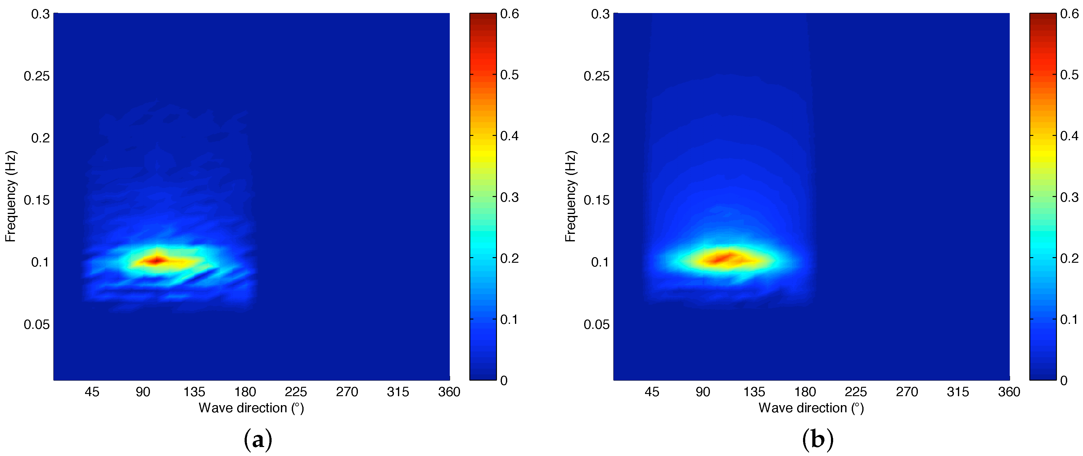
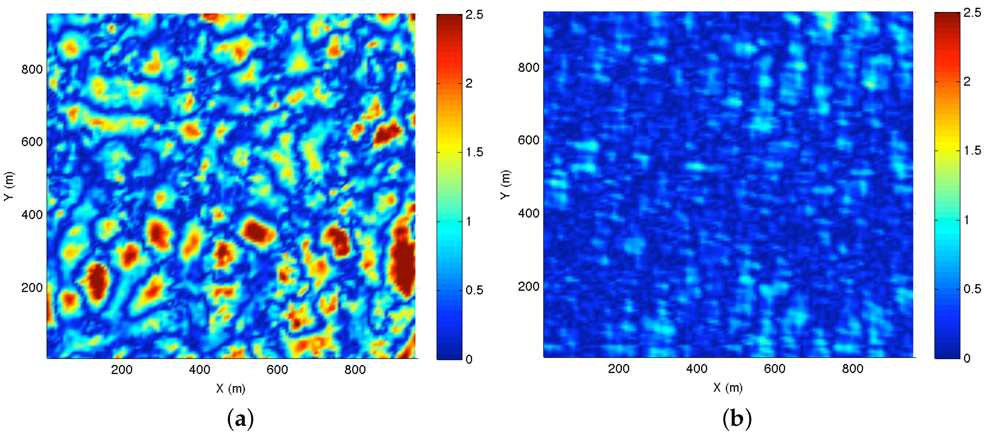
To verify the retrieved accuracy of the amplitude, the error between the simulated amplitude and the retrieved amplitude is presented in
Figure 3.
Figure 3a shows the error between the simulated amplitude and the amplitude retrieved by the 3D DFT method.
Figure 3b shows the error between the simulated amplitude and the amplitude retrieved by our method. From
Figure 2 and
Figure 3, it can be observed that the retrieved amplitude using the 3D DFT has a larger error than that of our method. Therefore, we can make the conclusion that our method has a relatively better performance than the 3D DFT method in terms of amplitude estimation.
Similarly, the phase of the individual wave components can be also retrieved with our method and the 3D DFT method.
Figure 4 presents the phase error of the retrieved individual wave components using these two methods. In order to better describe the phase error,
Figure 4 only presents the phase error of the dominant wave components, which means that the phase of individual wave component having a small amplitude is not taken into account. The difference between the simulated initial phase and the retrieved phase based on the 3D DFT method is given in
Figure 4a, while the difference between the simulated initial phase and the recovered phase based on our method is given in
Figure 4b. From
Figure 4, we can observe that the retrieved phase using 3D DFT method incurs larger errors than that of our successive cancellation method. Hence, we can say that our method also shows a relatively better performance than the 3D-DFT method in terms of phase estimation.
Despite the fact that we have compared the retrieved amplitude and phase between the 3D DFT method and our method, it is not reasonable to assess the performance only by these two parameters. On the other hand, the sea surface field based on the 3D DFT method can be reconstructed by the inverse 3D DFT on the wave spectrum or summing all the retrieved individual wave components, and the inverse 3D DFT method is more accurate than the other method [
11], since the superposition of the inaccurate wave components that are extracted by a traditional dispersion relation bandpass filter [
2,
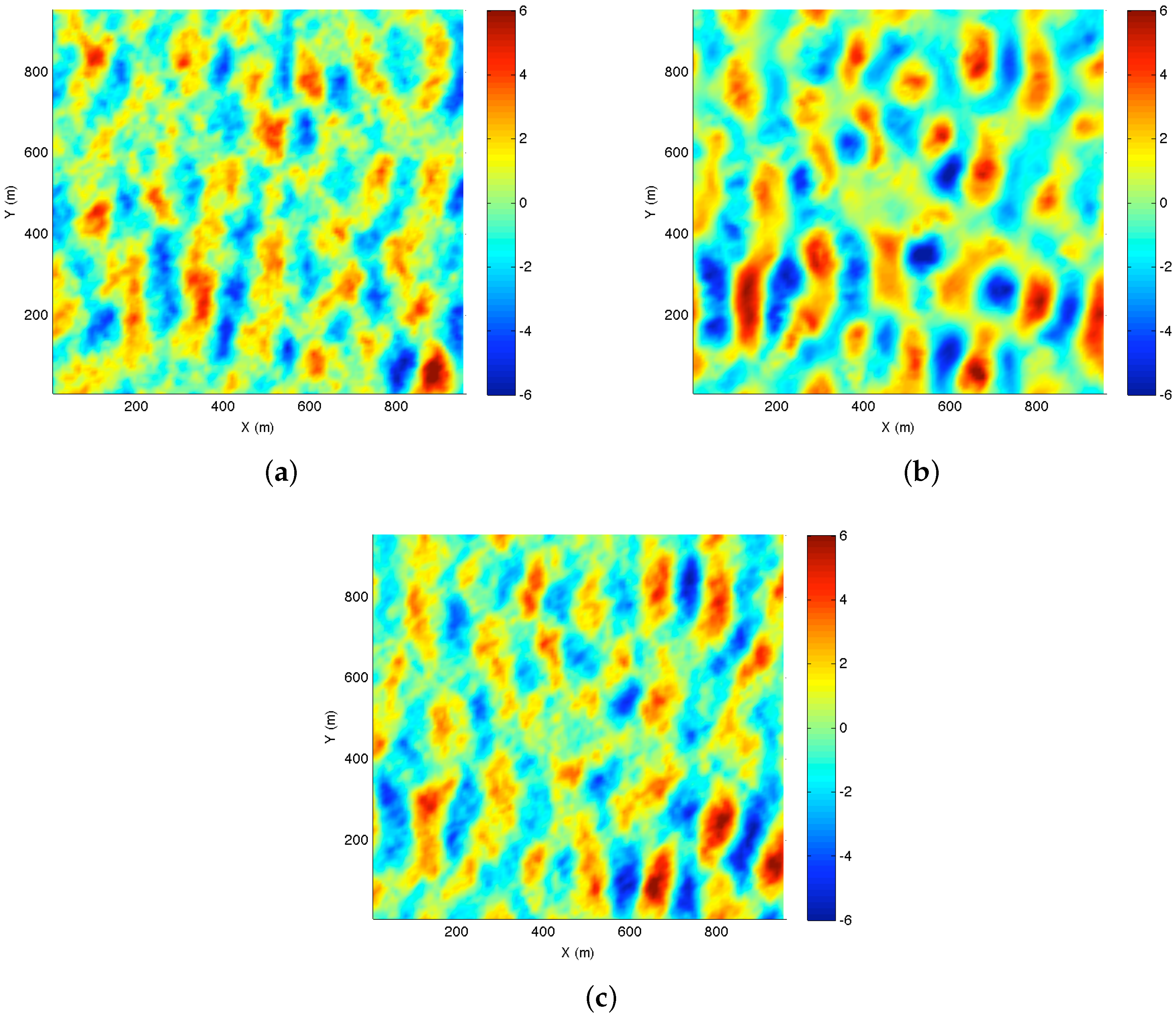
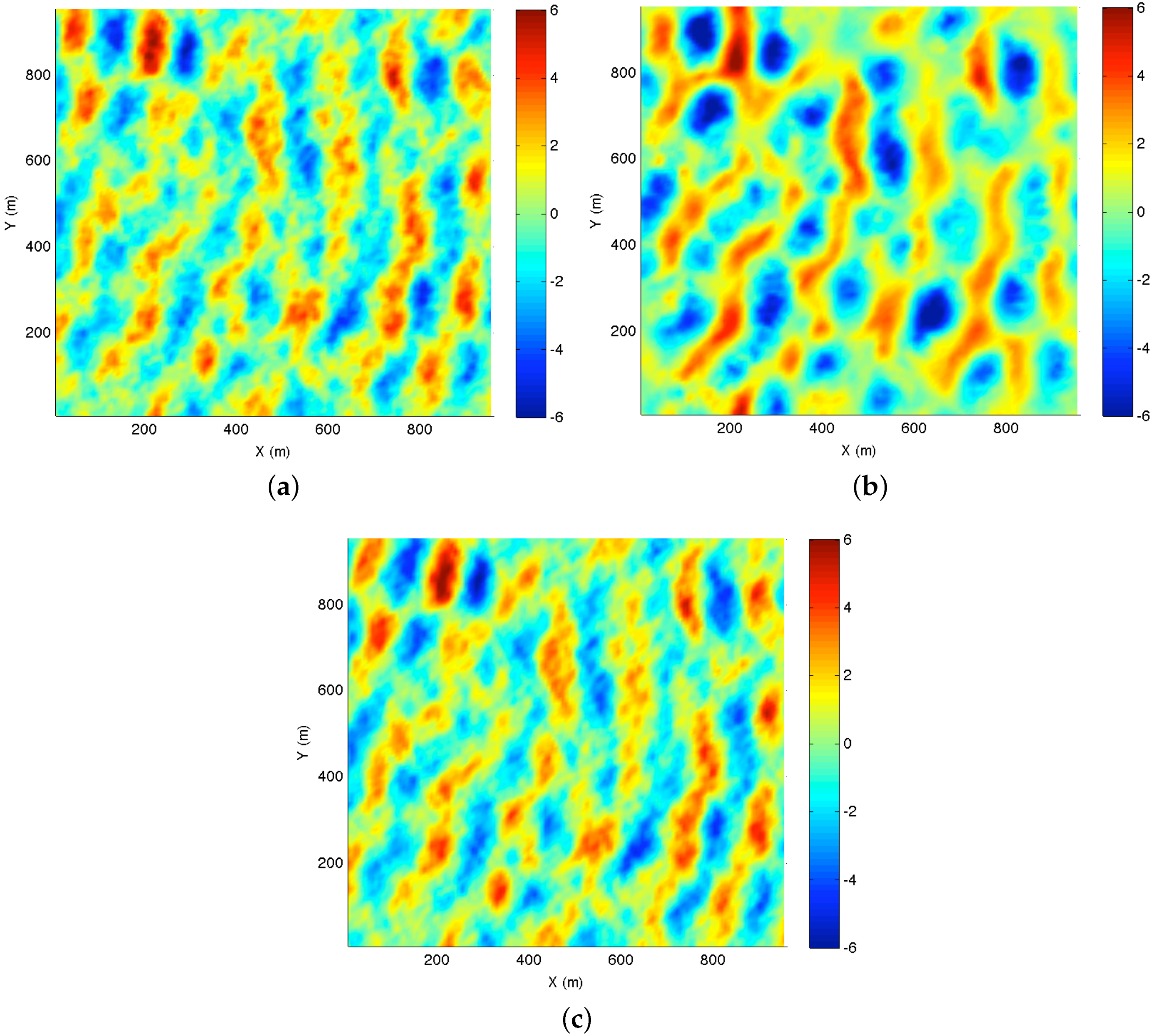
13] would deteriorate the reconstructed wave field. Hence, we can evaluate the performance of the retrieved wave components by the reconstructed field. To verify the effectiveness of our newly proposed algorithm, we only need to compare the sea surface field reconstructed by summing all individual wave components retrieved from our successive cancellation algorithm with that reconstructed by the inverse 3D DFT method on the wave spectrum after a bandpass filtering. The simulated wave field and the reconstructed wave fields described by these two methods at
s are given in
Figure 5.
Figure 5a is simulated wave field at
s using the amplitude in
Figure 1a. The red color denotes wave crest and the blue color represents wave trough.
Figure 5b shows the reconstructed sea surface field by the inverse 3D DFT method. The sea surface field reconstructed by summing all the individual wave components retrieved based on our successive cancellation method is presented in
Figure 5c. It is observed clearly that the reconstructed sea wave fields using the two methods are all similar to the simulated sea wave field in
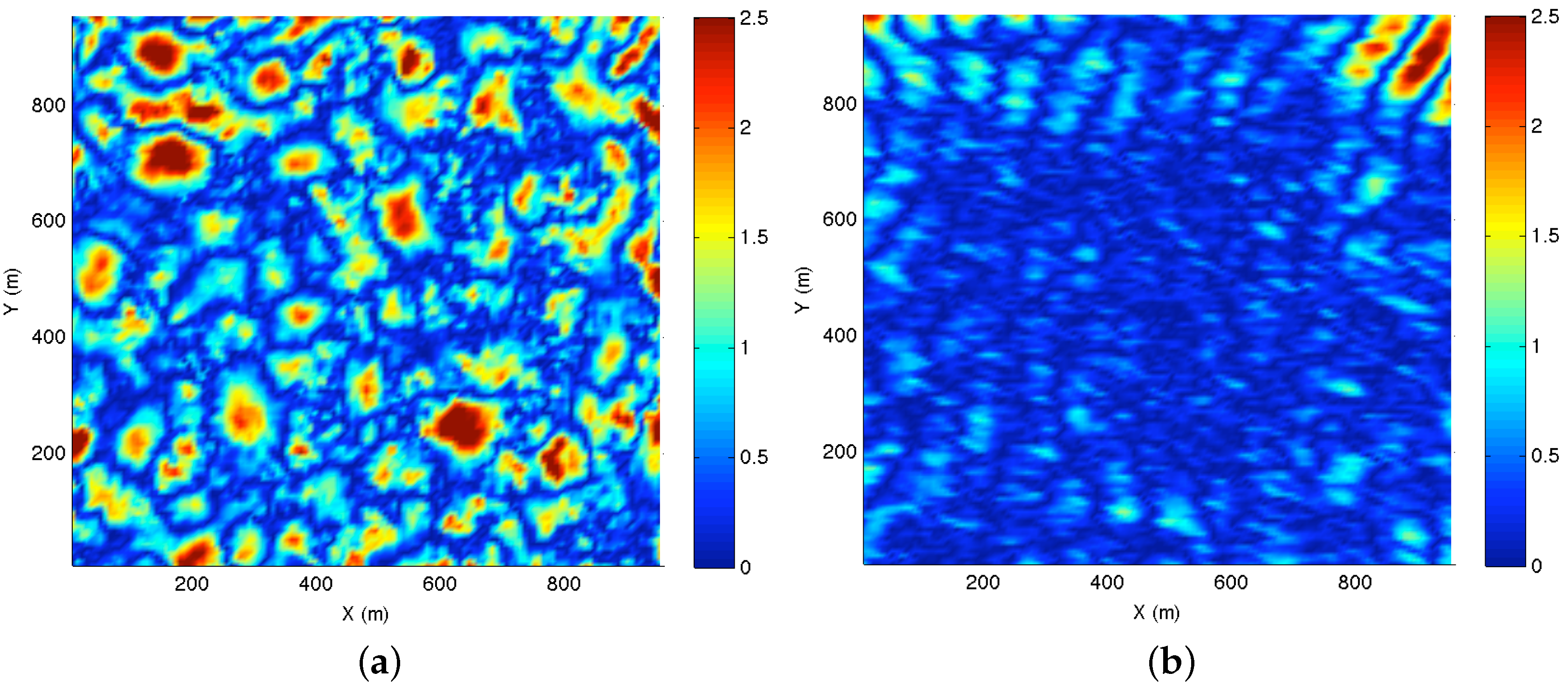
Figure 5a. In addition, the reconstruction error of the sea surface field of the two methods is shown in
Figure 6.
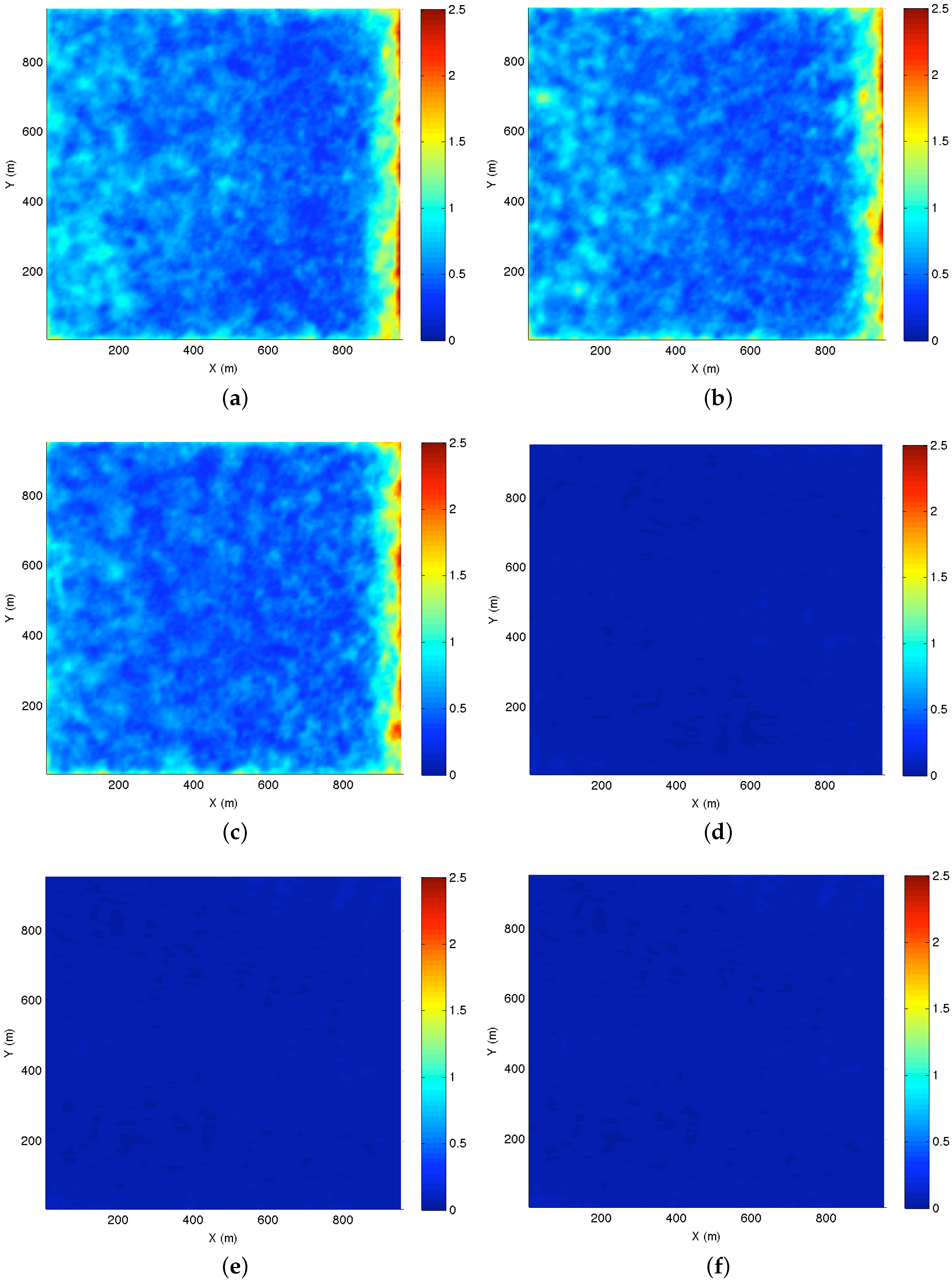
In order to further verify the validity of the proposed algorithm, 500 realizations with different sea states and directional resolution
are used. The average reconstruction error is expressed by
where
is the number of realizations,
and
represent the synthetic wave field and the recovered wave field, respectively and
denotes the average reconstruction error. Taking the synthetic wave image sequences as the ground truth, the average reconstruction error with the two methods are shown in
Figure 7 at three different times for
s,
s and
s.
Figure 7a–c show the average reconstruction error between the synthetic sea field and the recovered wave field with the 3D DFT method.
Figure 7d–f present the average reconstruction error between the synthetic sea field and the recovered wave field with our method. It can be observed that the reconstructed sea surface field using the retrieved individual wave components always shows a minor error compared with that of the inverse 3D DFT method at different times. It also implies that the successive cancellation method has a better performance in terms of exactly recovering sea wave components whose amplitudes and initial phases are almost successfully extracted using our method.
Since the 3D DFT method assigns energy to the components whose wavenumber
k and angular frequency
w do not necessarily satisfy the linear dispersion relation and the spectral leakage exists in both temporal and spatial domains, this results in the fact that the amplitude and initial phase extracted by the 3D DFT method have large errors [
3,
13,
14,
16,
17,
19,
26]. However, our new successive cancellation algorithm presents smaller error in extracting the wave components, since we attain
k from
w through the linear dispersion relation directly, which necessarily assures that our method has the capability to accurately extract wave components whose frequency and wavenumber rigorously satisfy the liner dispersion relation from the radar image sequence. In addition, in our method, the spectral leakage in the spatial domain is avoided, since we only take 1D DFT on the temporal domain and apply the successive cancellation algorithm in the spatial domain, which is alternative to the 2D DFT method.
4.3. The Experiment with High Directional Resolution
When the more wave directions are taken in the directional wave spectrum, the angular frequency and the wave component direction are uniformly discretized with
rad/s and
, respectively. The simulated amplitude and the recovered amplitude are given in
Figure 8.
Figure 8a is the simulated amplitude based on the JoNSWaP spectrum. The amplitude recovered with our method is shown in
Figure 8b. With the increase of the directional resolution, the experiment shows that it is unable to resolve all the directions, since the directions are too close to be resolved using our method. It can be seen that not all the amplitudes can be recovered and the recovered amplitude presents an obvious error. In practice, there is an large error in the retrieved phase, which is not presented here.
In spite of the fact that our method is unable to recover every wave component, the reconstructed sea field using the obtained inaccurate wave components is also presented. The simulated sea field and reconstructed sea surface field with the two methods at
s are shown in
Figure 9.
Figure 9a is the simulated sea field at
s. The recovered sea field with the inverse 3D DFT method is shown in
Figure 9b.
Figure 9c is the reconstructed sea field by summing all the attained inaccurate wave components based on our method. The result is interesting, since the reconstructed sea surface field based on our method is in accordance with the simulated sea field in
Figure 9a as well as that based on the inverse 3D DFT method in
Figure 9b. Moreover, the reconstruction error of the two methods is shown in
Figure 10. The experimental result is that the reconstruction error of our proposed method is smaller than that of the inverse 3D DFT method, which is the same as the above in
Figure 8.
Therefore, when more wave directions are taken in the directional wave spectrum, the experiment shows that our method fails to resolve all the directions of the individual wave components, since the directions are too close to be resolved using the successive cancellation method. However, the reconstructed sea surface field is still accurate. Based on the experimental result, we conjecture that each retrieved inaccurate wave component might be the superposition of a few of wave components simulated in some certain range of angles.
4.4. Results Analysis
The accuracy of our method is investigated by analyzing the extracted wave components and the sea wave field that is reconstructed by the sum of all the achieved wave components. Under the condition of low directional resolution, the experiments above show that our proposed successive cancellation algorithm is capable of accurately extracting the parameters of the wave component including the amplitude and phase from the simulated sea wave image sequences, which has less error than that of the 3D DFT method. With high directional resolution, our method can still accurately reconstruct the sea wave field. However, it should be mentioned clearly that these results are based on the perfect data. The accuracy and effectiveness of our algorithm are verified with a rather generic and idealized test. Therefore, more experiments are needed to verify its accuracy in various sea conditions.


