A Spatial Downscaling Algorithm for Satellite-Based Precipitation over the Tibetan Plateau Based on NDVI, DEM, and Land Surface Temperature

Abstract

Precipitation is an important controlling parameter for land surface processes, and is crucial to ecological, environmental, and hydrological modeling. In this study, we propose a spatial downscaling approach based on precipitation–land surface characteristics. Land surface temperature features were introduced as new variables in addition to the Normalized Difference Vegetation Index (NDVI) and Digital Elevation Model (DEM) to improve the spatial downscaling algorithm. Two machine learning algorithms, Random Forests (RF) and support vector machine (SVM), were implemented to downscale the yearly Tropical Rainfall Measuring Mission 3B43 V7 (TRMM 3B43 V7) precipitation data from 25 km to 1 km over the Tibetan Plateau area, and the downscaled results were validated on the basis of observations from meteorological stations and comparisons with previous downscaling algorithms. According to the validation results, the RF and SVM-based models produced higher accuracy than the exponential regression (ER) model and multiple linear regression (MLR) model. The downscaled results also had higher accuracy than the original TRMM 3B43 V7 dataset. Moreover, models including land surface temperature variables (LSTs) performed better than those without LSTs, indicating the significance of considering precipitation–land surface temperature when downscaling TRMM 3B43 V7 precipitation data. The RF model with only NDVI and DEM produced much worse accuracy than the SVM model with the same variables. This indicates that the Random Forests algorithm is more sensitive to LSTs than the SVM when downscaling yearly TRMM 3B43 V7 precipitation data over Tibetan Plateau. Moreover, the precipitation–LSTs relationship is more instantaneous, making it more likely to downscale precipitation at a monthly or weekly temporal scale.

1. Introduction

Precipitation is a key factor of ecological, hydrological, and climatological models that reflect surface environmental conditions and the global water cycle [1,2], in addition to basic observations in meteorological datasets. Most land surface processes are controlled by precipitation, making it an important surface meteorological input parameter in various types of models of plant physiology, ecology, hydrology, and other fields [3,4,5,6]. Thus, attaining accurate and high resolution precipitation data is critical for understanding land surface processes and global climate change. Although observations from meteorological stations and rain gauges have long temporal series records and are important methods for acquiring precipitation data, acquiring precipitation observations over mountainous and underdeveloped areas remains a great challenge owing to the sparse rain gauge network [7,8,9]. Over the past three decades, development of satellite sensors has resulted in multiple sources of precipitation datasets [10,11,12,13] that provide more reliable estimations of precipitation over un-gauged areas compared with various interpolation methods. However, their spatial resolutions (i.e., 0.25–5°) are still too coarse for hydrological simulation and environmental modeling when applied to local basins and regions [14,15].

During the past decades, many attempts have been made to map fine spatial resolution precipitation from satellite-based remote sensing precipitation data. Great efforts have been made to advance the spatial downscaling algorithms of satellite-based precipitation datasets based on the relationship between precipitation and land surface characteristics. Immerzeel et al. [14] proposed an algorithm for downscaling Tropical Rainfall Measuring Mission (TRMM)-based annual precipitation datasets from 0.25° to 1 km by using the exponential function between the precipitation and Normalized Difference Vegetation Index (NDVI). Jia et al. [15] improved the algorithm by using multiple linear regression model and introduced both NDVI and Digital Elevation Model (DEM) as independent variables, downscaling the TRMM 3B43-derived annual precipitation data in the Qaidam Basin of China to 1 km × 1 km resolution. Chen et al. [16] and Xu et al. [17] constructed a geographically weighted regression model based on the assumption that the rainfall–geospatial factors relationship varies spatially but is similar in a region. Shi et al. [18] proposed a downscaling algorithm by introducing a machine learning algorithm known as Random Forests (RF) for detecting the complex precipitation–NDVI and precipitation–DEM relationships. Their validation results indicated that the Random Forests-based downscaling model outperformed compared to the linear regression and the exponential regression models. These approaches have improved the downscaling accuracy for satellite-based precipitation data. Thus, more advanced algorithms have been introduced for constructing a precipitation–vegetation index and precipitation–topography relationships, which has in turn expanded the application of satellite-based precipitation downscaling approaches. However, notable problems remain. Recent downscaling models are based mainly on the relationships of vegetation index–precipitation and terrain features–precipitation; therefore, satellite precipitation datasets over regions with no relationship with NDVI and DEM could not be downscaled with these algorithms. For example, in barren areas or deserts, the precipitation does not affect the NDVI owing to the sparse distribution of vegetation [17].

The purpose of this study is to obtain annual total precipitation maps with fine spatial resolution from coarse resolution satellite-based precipitation datasets, for which we proposed a spatial downscaling method based on the researches of Immerzeel et al., Jia et al., and Shi et al. [14,15,18]. In this study, we introduced land surface temperature as a factor for enhancing the precipitation–land surface characteristics relationships when downscaling annual total precipitation data. Considerable relationships have been observed and detected between land surface temperature and precipitation [19], even in regions with no precipitation–NDVI relationship. Precipitation could change the local land surface temperature both in the daytime and at night; rain results in cooler temperatures, whereas droughts are often accompanied by heat waves [20]. In this study, we used land surface temperature in both daytime and nighttime and the day–night temperature difference, NDVI, and DEM as independent input variables for downscaling the yearly TRMM 3B43 V7 precipitation dataset over the Tibetan Plateau from 2001 to 2010.

Machine learning techniques have been widely used in remote sensing images processing, land cover classification, and land surface parameters derivation [4,21,22], and are distinguished in dealing with complex and non-linear problems [23]. In this study, we tested two machine learning algorithms: Random Forests (RF) and Support Vector Machine (SVM).

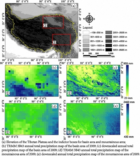
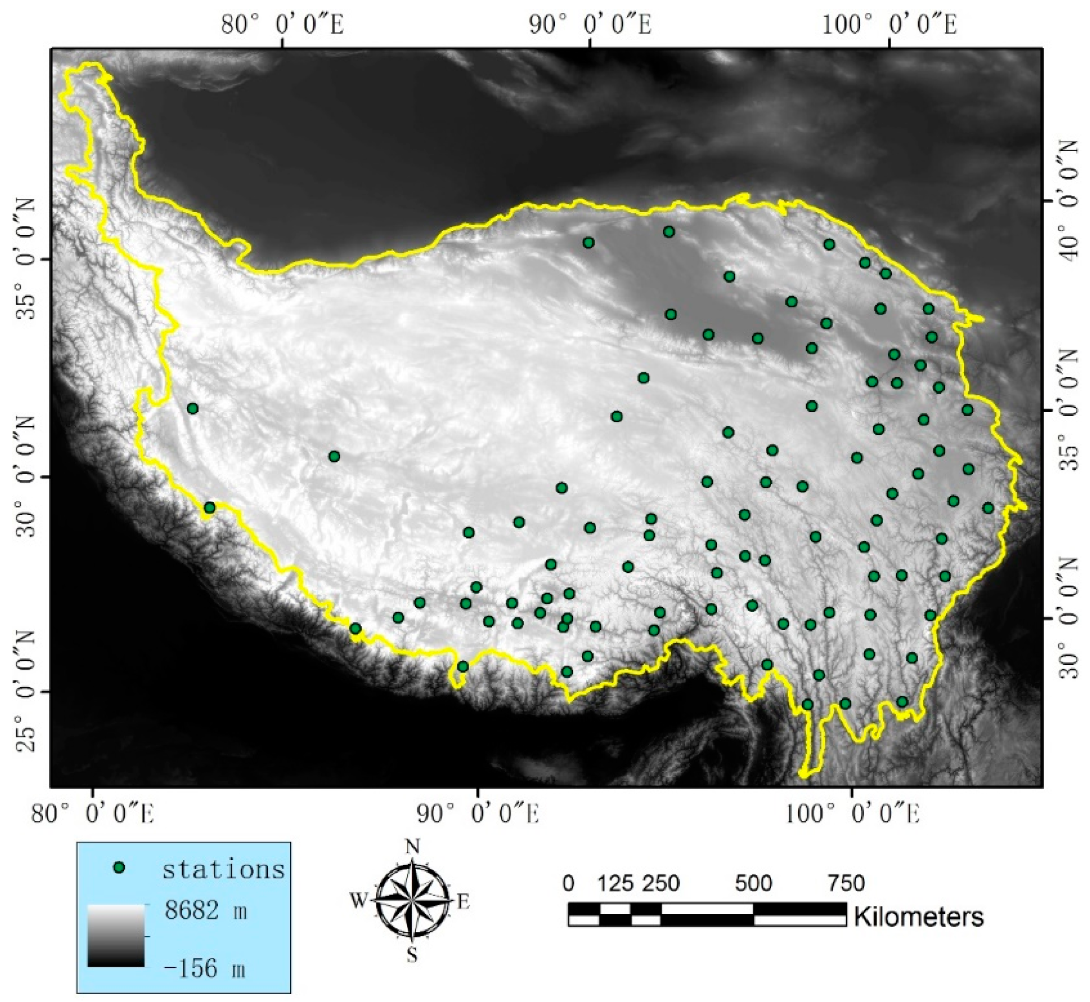
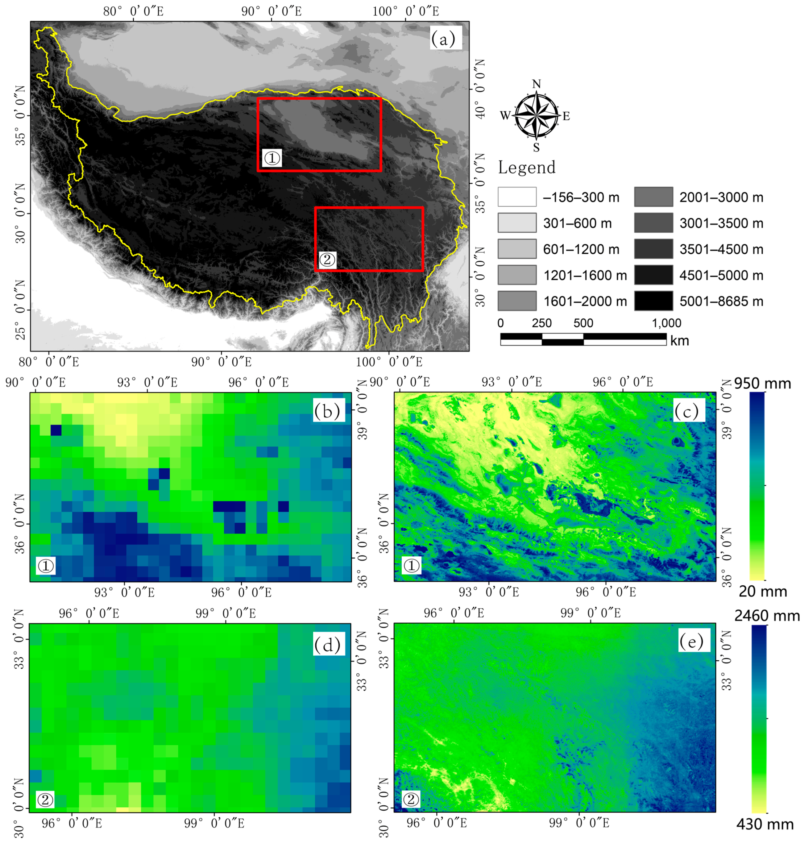
2. Study Area and Data Resources

The Tibetan Plateau is a vast elevated plateau in Central Asia and East Asia, covering most of the Tibet Autonomous Region and Qinghai Province in western China [24]. It stretches about 1532 km north to south and 2945 km east to west, covering a total area of 2572.4 × 10³ km² between 26°00′12′′N and 39°46′50′′N and 73°18′52′′N and 104°46′59′′N (Figure 1) [24]. The spatial distributions of 93 rain gauge stations in the study area are presented in Figure 1. These stations are located mostly in the eastern part of the area and are sparse over the western part of the Tibetan Plateau. The observation records data were provided by the National Meteorological Information Center [25].

The Tropical Rainfall Measuring Mission (TRMM) is a joint mission of NASA and the Japan Aerospace Exploration Agency that was launched in 1997 to study rainfall for weather and climate research. TRMM is a research satellite designed to improve our understanding of the distribution and variability of precipitation covering the tropical and sub-tropical regions of the earth and has provided much needed information on rainfall and its associated heat release [13]. The TRMM 3B43 product provides monthly precipitation data at a spatial resolution of 0.25° × 0.25°, covering 50°N–50°S. Version 7 of TRMM 3B43 (TRMM 3B43 V7) from January to December between 2001 and 2010 was used in this study; these data were downloaded from the National Aeronautics and Space Administration (NASA) Precipitation Measurement Missions (PMM) website [26]. The annual total precipitation was calculated by accumulating monthly precipitation from January to December. The original TRMM 3B43 V7 data were reprojected to the Albers Conical Equal Area projection and resampled to 25-km resolution using the nearest neighbor resampling algorithm during the reprojection. The nearest neighbor resampling algorithm was used because it would not alter the value of the original sensed data.

Two MODIS products, monthly NDVI (MOD13A3) and land surface temperature (MOD11A2), were downloaded from the NASA Land Processes Distributed Active Archive Center (LP DAAC) [27]. These two products, having a sinusoidal projection, were reprojected to the Albers Conical Equal Area projection. The nearest neighbor resampling algorithm was used to resample MODIS NDVI images to maintain the pixel size of 1 km × 1 km. MOD11A2 is composed of daytime and nighttime land surface temperature variables (LSTs) at a time interval of eight days; the annual average LSTs were calculated by averaging each eight-day LST.

The DEM data used in this study were obtained from the NASA Shuttle Radar Topographic Mission (SRTM) [28]. Two spatial resolutions, 30 m and 90 m, DEM were available. Considering the spatial scales of this study, we downloaded the DEM data with a spatial resolution of 90 m and then resampled them to 1 km by averaging the values of all pixels within each 1-km pixel.

3. Methods

3.1. Downscaling Methodology

The spatial downscaling method is based on the relationship between precipitation and land surface characteristics. The basic concept of the downscaling method is to model the relationship between precipitation and land surface characteristics at coarse resolution; then the established model is applied to the fine spatial resolution land surface characteristics data to achieve precipitation at fine spatial resolution. For downscaling the TRMM 3B43 V7 precipitation data, we used five land surface characteristics as independent variables, NDVI, DEM, daytime land surface temperature (LST_day), nighttime land surface temperature (LST_night), and day–night land surface temperature difference (LST_DN). Two machine learning algorithms, RF and SVM, were implemented to detect the possible relationships between precipitation and land surface characteristics. Meanwhile, the exponential regression (ER) model proposed by Immerzeel et al. [14] and multiple linear regression (MLR) model proposed by Jia et al. [15] were also used for comparison purposes. The process of the downscaling model proposed in this study is based on the research of Jia et al. and Immerzeel et al. [14,15]. The process is described below:

(1)

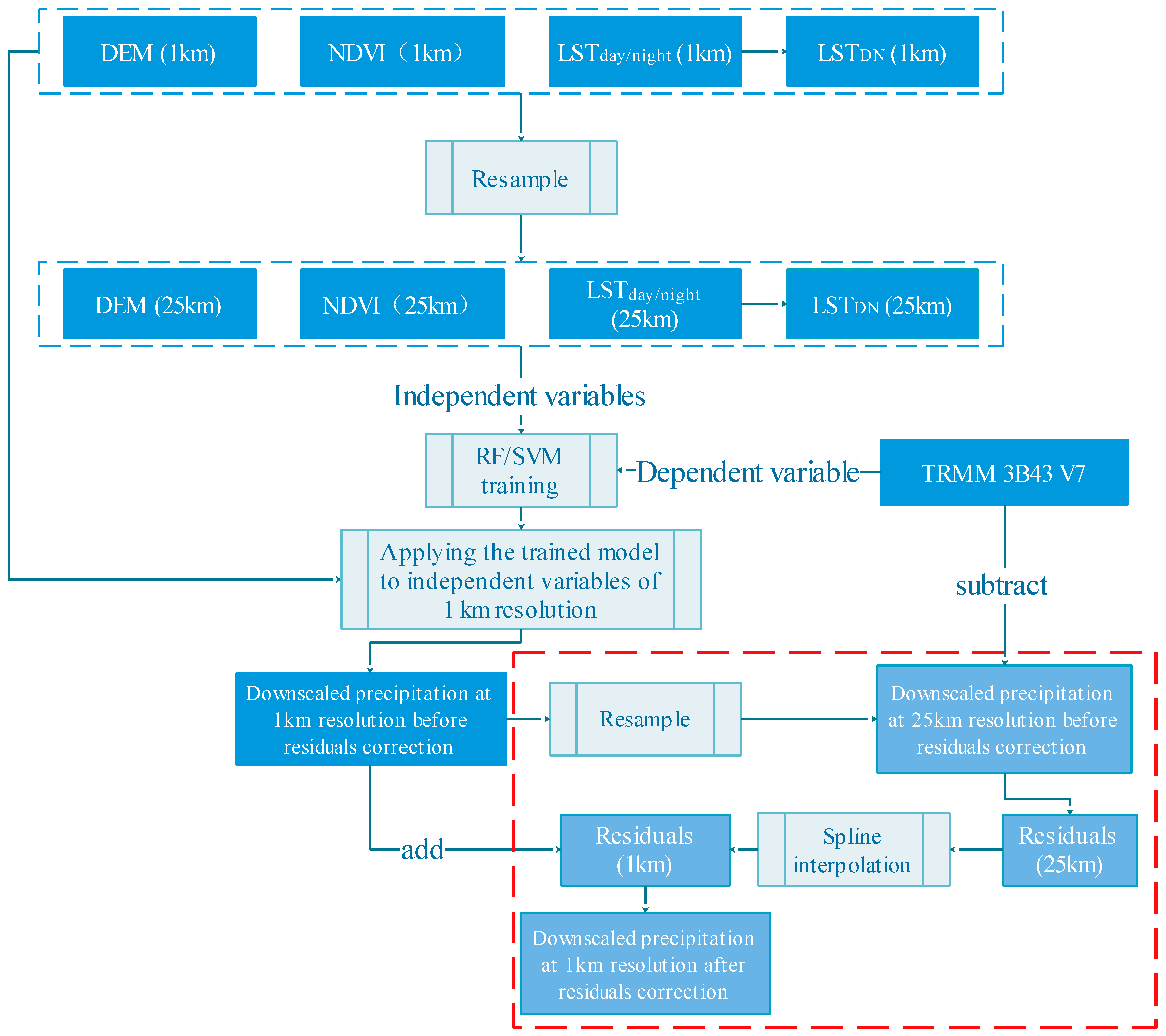
In regions with snow, water bodies, and desert cover, the NDVI values are usually constant under 0.0. To eliminate the influences of snow and water bodies, the threshold NDVI < 0.0 was used to distinguish and remove the snow and water body pixels from the original monthly NDVI images. Then, the average annual NDVI was calculated by averaging the monthly NDVI from January to December.

(2)

The LST_DN is calculated by subtracting LST_night from LST_day. NDVI_1km, DEM_1km, LST_day-1km, LST_night-1km, and LST_DN-1km are resampled to 25-km resolution by averaging all 1-km pixel values in each 25-km pixel. We used the average algorithm because the average value represents the overall situation within each 25-km pixel, and can reduce the influence of the outliers among the 1-km pixels.

(3)

The relationship between re-sampled independent variables and TRMM 3B43 V7 precipitation data is established by using the SVM and RF algorithms. The RF and SVM algorithms are implemented in scikit-learn, which is a Python package integrating a wide range of state-of-the-art machine learning algorithms for medium-scale supervised and unsupervised problems [29].

(4)

High spatial resolution (1 km) variables are input into the models established in Step (3). Downscaled precipitation at 1 km resolution (PRE_1km) is then achieved.

(5)

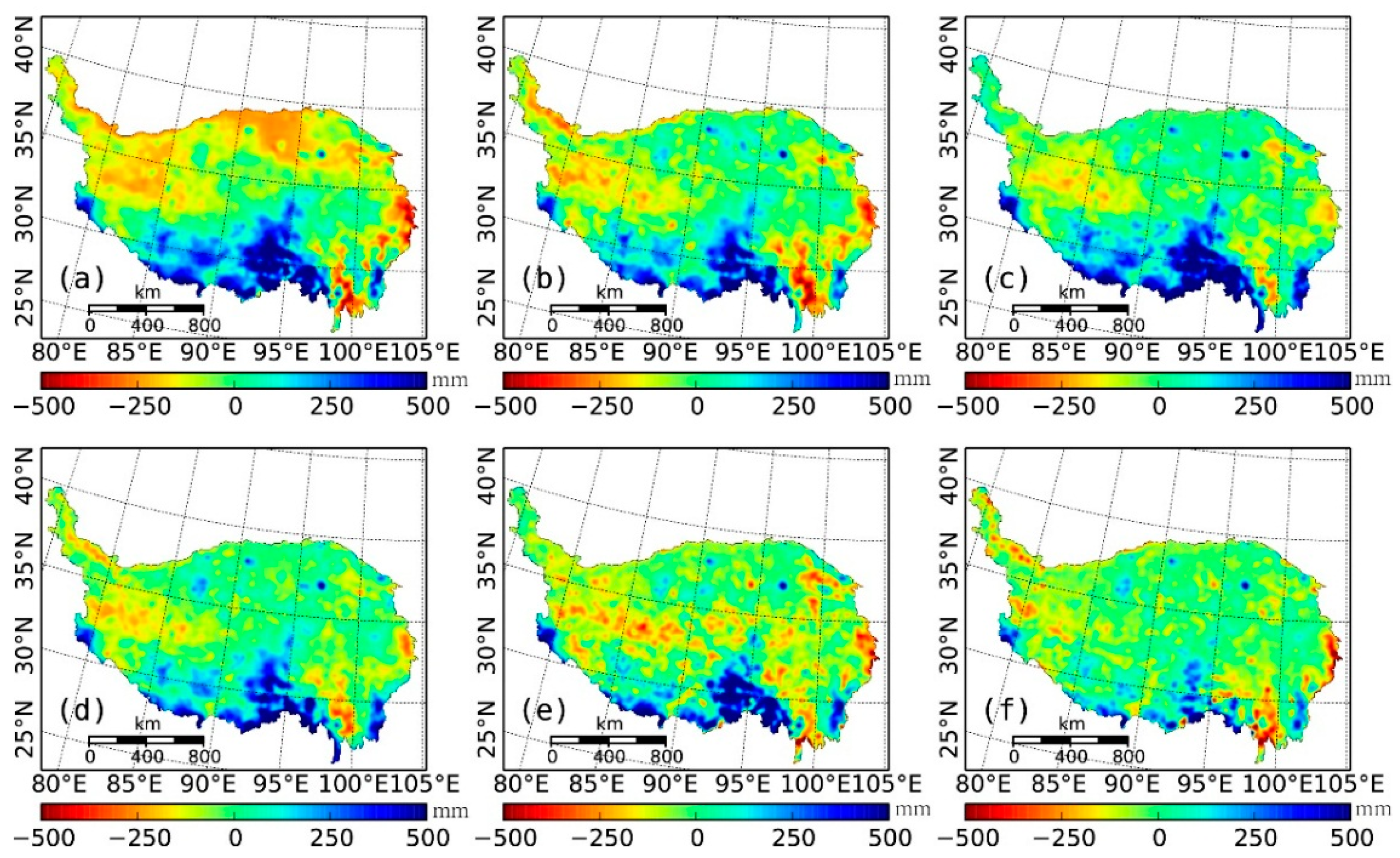
Residual correction is an essential step for the downscaling method based on statistical algorithms that can correct the precipitation that could not be predicted by the models. The PRE_1km are resampled to 25 km by averaging all 1-km pixel values in each 25-km pixel. Then the residuals of the models are calculated by subtracting the resampled PRE_1km from the original TRMM data.

(6)

The residuals are interpolated by using a simple spline tension interpolator to 1 km spatial resolution. Splining is a deterministic technique to represent two-dimensional curves on three-dimensional surfaces. It assumes smoothness of variation, and is typically used for regularly-spaced data [14,15]. The corrected downscaled precipitation results (PRE_C-1km) are then obtained by adding the interpolated residual to PRE_1km.

In this section, a flowchart was provided to illustrate the main steps of the downscaling algorithm (Figure 2). It should be noted that NDVI_1km, DEM_1km, and LST_1km have been pre-processed according to Steps (1) and (2). The steps in the red rectangle are the residual correction described in Steps (5) and (6).

3.2. Brief Description of Support Vector Machine

Support Vector Machine (SVM) is an outstanding machine learning algorithm for classification and regression problems and has been successfully applied in different fields such as soil moisture estimation [4], impervious surface estimation [30], and biophysical parameter estimation from remote sensing data [31]. The original SVM algorithm was invented by Vladimir Vapnik and his co-workers in the early 1990s for classification problems, and then was extended to the case of regression [32,33]. The basic concept of the SVM algorithm is derived from optimization theory, which uses a hyperplane to classify the input variables into an m-dimensional feature space with maximal margin. The maximal margin is derived by solving a constrained quadratic problem:

$$\text{Maximize W}\left(\mathsf{\alpha }\right)={\displaystyle \sum }_{i=1}^n{\mathsf{\alpha }}_i-\frac{1}{2}{\displaystyle \sum }_{i=1}^n{\displaystyle \sum }_{j=1}^n{\mathsf{\alpha }}_i{\mathsf{\alpha }}_j{y}_i{y}_{j}K\left(x_i,x_j\right)$$

(1)

$$\text{Subject to }\left\{{{\displaystyle \sum }}_{i=1}^n{\mathsf{\alpha }}_i{y}_i=0 and 0\le {\mathsf{\alpha }}_i \le C for i=1, 2, \dots n\right\},$$

(2)

where $x_i\in R_d$ are the training sample vectors, and $K\left(x_i,x_j\right)$ is the kernel function.

$$f\left(x,\mathsf{\omega }\right)= {{\displaystyle \sum }}_{j=1}^m{\mathsf{\omega }}_j{g}_j\left(x\right)+b,$$

(3)

where $g_j\left(x\right)$, j = 1, 2, …, m denotes a set of nonlinear transformations, and b is the “bias” term.

3.3. Brief Description of Random Forests

Random Forests (RF), a non-parameter and ensemble learning algorithm for regression and classification, has been increasingly applied because it yields high accuracy and is robust to outliers [21]. RF, which was proposed by Breiman [34], is a combination of tree predictors such that each tree depends on the values of a randomly chosen subset of input variables vectors sampled independently and with the same distribution for all trees in the forests [34]. The tree predictor is based on the classification and regression trees (CART) algorithm [35], in which the basic concept is to construct a tree-like graph or model of decisions and their possible consequences by generating relative homogeneous subgroups by recursively partitioning the training dataset to the maximum variance between groups of independent variables and dependent variables in each of the terminal nodes of the tree. A simple and accurate model is built to explain the relationship of independent and dependent variables. The RF regression algorithm process can be briefly described as follows:

(1)

The ntree (number of trees) samples set is randomly drawn from the original training sample set with replacement. Each sample set is a bootstrap sample, and the elements that are not included in the bootstrap are termed out-of-bag data (OOB) for that bootstrap sample.

(2)

For each bootstrap sample, an un-pruned regression tree is grown with the modification that, at each node, a random subset of the variables is selected from which the best variables are split.

(3)

Predictions for new samples can be made by averaging the predictions from all the individual regression trees:

$$f= \frac{1}{N} {{\displaystyle \sum }}_{i=1}^N{f}_i\left(x\right),$$

(4)

where N is the number of trees and $f_i\left(x\right)$ is the prediction from each individual regression tree.

The ranking of variable importance is an important issue in the RF algorithm. During the fitting process, the prediction error for each out-of-bag (OOB) sample is recorded and averaged over the forest. To measure the importance of the i-th variable, the values of that variable are permuted while keeping the values of other independent variables unchanged. Then the OOB error is again computed on this perturbed dataset. The importance score for the i-th variable is computed by averaging the difference in out-of-bag (OOB) error before and after the permutation over all trees. These variable importance values are then used to rank the order of those independent variables in terms of their contributions to the regression model.

3.4. Exponential Regression (ER) and Multiple Linear Regression (MLR) Models

The exponential regression (ER) model proposed by Immerzeel et al. [14] and multiple linear regression (MLR) model proposed by Jia et al. [15] were also used for downscaling the TRMM 3B43 V7 data. These algorithms can be briefly described as follows:

(1)

Exponential regression (ER) model:

The exponential regression (ER) model [14] is based on the vegetative response to TRMM precipitation. An exponential regression is performed between NDVI and the TRMM 3B43 V7 data as shown in Equation (1):

$$\mathrm{P}=\mathrm{a}\ast e^{\mathrm{b}\ast \mathrm{NDVI}},$$

(5)

where P is the TRMM precipitation, and a and b are the fitting coefficients of the exponential regression model.

(2)

Multiple linear regression (MLR) model:

Jia et al. [15] used an MLR model for fitting the relationships of TRMM precipitation with NDVI and elevation, downscaling the TRMM precipitation data to a fine spatial resolution. In this study, we constructed the MLR model with NDVI, DEM, and LSTs as independent variables:

$$\mathrm{P}=a_1\ast \mathrm{NDVI}+ a_2\ast \mathrm{DEM}+a_3{\mathrm{LST}}_{day}+a_4{\mathrm{LST}}_{night}+ a_5{\mathrm{LST}}_{DN}+\mathrm{c},$$

(6)

where $a_1$, $a_2$, …, $a_n$ are the slopes of each independent variable, and c is the intercept of the regression function.

3.5. Validation

Validation of the downscaled results is based on the ground observation from 93 independent meteorological stations distributed over the study area. First, three comparison criteria were calculated, the coefficient of determination (R²), the mean absolute error (MAE), and the root mean squared error (RMSE), which are expressed as:

$$R^2=\frac{\left\{{{\displaystyle \sum }}_{k=1}^n\left[\left(Y_k-\overline{Y}\right)\left(O_k-\overline{O}\right)\right]\right\}}{\sqrt{\left[{{\displaystyle \sum }}_{k=1}^n{\left(Y_k-\overline{Y}\right)}^2\right]}\sqrt{\left[{{\displaystyle \sum }}_{k=1}^n{\left(O_k-\overline{O}\right)}^2\right]}}$$

(7)

$$\text{MAE}={\displaystyle \sum }_{k=1}^n\left|\left(Y_k-O_k\right)\right|/n$$

(8)

$$\text{RMSE}= \sqrt{{{\displaystyle \sum }}_{k=1}^n{\left(Y_k-O_k\right)}^2/n},$$

(9)

where $Y_k$ is the observation measured by station k, $O_k$ is the precipitation estimated by a model at the location of station k, $\overline{Y}$ is the mean value of all station observations, and $\overline{O}$ is the mean value of the estimated precipitation at all the locations with stations.

In addition, we also compared the cumulative distribution function (CDF) curve of the downscaled results derived at the locations of stations with observations measured by the stations. The CDF represents the distribution as the percentage of occurrences of each value, expressed as:

$$\mathrm{Pr}\left(\mathrm{X}<x^{\prime }\right)=F\left(x^{\prime }\right)={{\displaystyle \sum }}_{k=1}^{n}f\left(x_k\right)$$

(10)

where $x_k$ is the largest discrete value of $X$ less than or equal to $x^{\prime }$.

4. Results and Analysis

The TRMM 3B43 V7 data from 2001 to 2010 over the Tibetan Plateau were downscaled from 0.25° to 1 km using algorithms proposed by Immerzeel et al. [14] and Jia et al. [15] and the algorithm based on SVM and RF. In this study, we introduced land surface temperature as an independent variable to investigate whether these factors are beneficial for downscaling algorithms. The SVM- and RF-based downscaling algorithms were performed with only the combination of NDVI and DEM and the combination of NDVI, DEM, and LSTs (daytime, nighttime, and day–night difference), respectively. The algorithms proposed by Immerzeel et al. [15] and Jia et al. [15] were termed as ER and MLR, whereas the SVM- and RF-based algorithms with NDVI and DEM and with a combination of NDVI, DEM, and LST were termed SVMND, SVMNDL, RFND, and RFNDL, respectively.

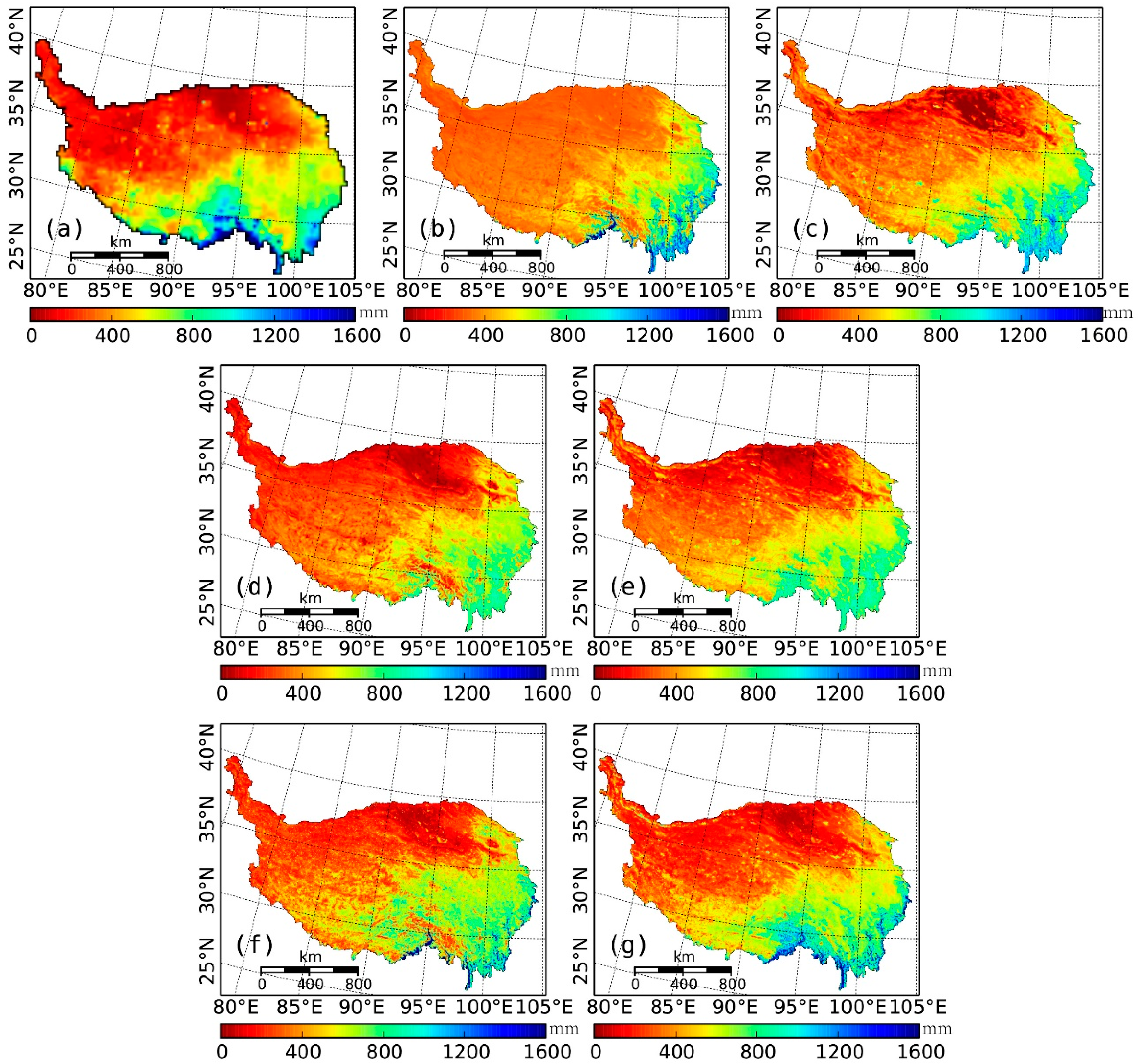
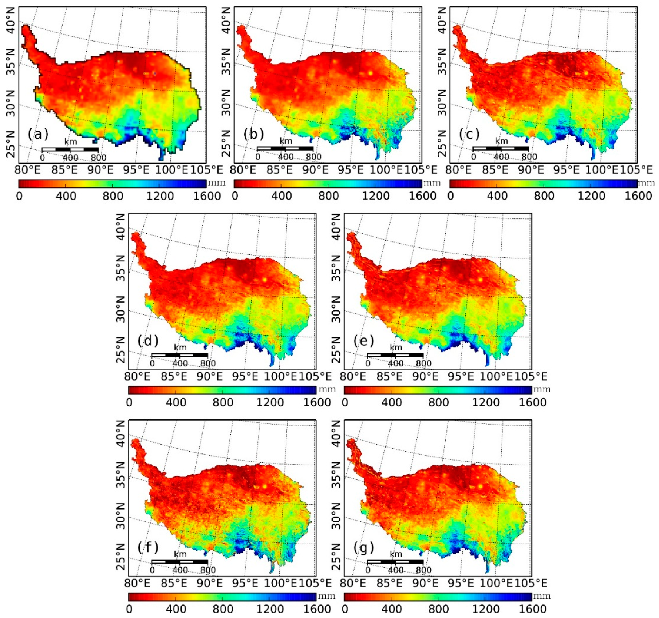
4.1. Downscaled Results

The establishment of the RF- and SVM-based models depended largely on certain parameterizations. The choice of optimal parameters is significant. In practice, we conducted experiments to cover a majority range of parameter combinations for each algorithm (

Table 1. Parameter combinations for each algorithm.

Algorithm	Abbreviation	Parameter Type	Parameter Set
Random Forests	RF	NumTrees	20, 40, 60, 80, 100,120, 140, 160, 180, 200, 220, 240, 260, 280, 300
Support Vector Machine	SVM	kernelType	Radial basis function
		Cost	10, 20, 30, 40, 50, 60, 70, 80, 90, 100
		gamma	2−4, 2−3, 2−2, 2−1, 1, 21, 22, 23, 24

), and a grid search algorithm was implemented to find the optimal parameters for each algorithm. It should be noted that the NDVI, DEM, and LSTs were all input into the MLR model as independent variables, and a stepwise regression was used for establishment of that model.

Figure 3 presents the R², MAE, and RMSE estimated by model for each year. It should be noted that a grid search was conducted to find the optimal parameters for each year. In general, the RF-based model produced the highest R² and the lowest MAE and RMSE, followed the SVMDNL model. However, the RFNDL and SVMNDL simulated a higher R² and a lower MAE and RMSE than RFND and SVMND, respectively. This indicates that the inclusion of LSTs is beneficial for increasing model accuracy.

Figure 4 shows the TRMM 3B43 V7 product over the Tibetan Plateau in 2008 (Figure 4a) and the downscaled results using the ER, MLR, SVMND, SVMNDL, RFND, and RFNDL before residual correction. The results of ER before residual correction show a significantly different spatial distribution pattern compared with the original TRMM 3B43 V7, whereas the downscaled results of MLR, RFND, RFNDL, SVMND, and SVMNDL have spatial distribution patterns similar to those of TRMM 3B43 V7.

The residuals of the ER, MLR, SVM, and RF were calculated using the approach described above. Figure 5 shows the residuals interpolated by using the spline tension interpolator. The spatial distribution of the residual of ER model indicated that it tends to underestimate the TRMM 3B43 V7 precipitation over the southern part of the Tibetan Plateau and overestimate values over most of the other parts of the study area. The MLR tended to underestimate the southern part and overestimate the eastern and western parts of the area. The residuals of SVMND and SVMDNL present a spatial distribution pattern similar to that of MLR. In contrast, the residual of the RFNDL presents an irregular spatial distribution pattern.

Figure 6 shows the downscaled precipitation data after residual correction. Compared with the downscaled results without residual correction (Figure 4), the downscaled result of the ER model after residual correction are more likely to show the similar spatial distribution pattern of the original TRMM 3B43 V7. The downscaled results of the MLR, SVMND, and SVMNDL after residual correction tended to be higher over the southeast Tibetan Plateau, which agreed with the original TRMM 3B43 V7. In contrast, the downscaled result of the RFNDL after residual correction showed little change compared with that before residual correction.

4.2. Validation and Error Analysis

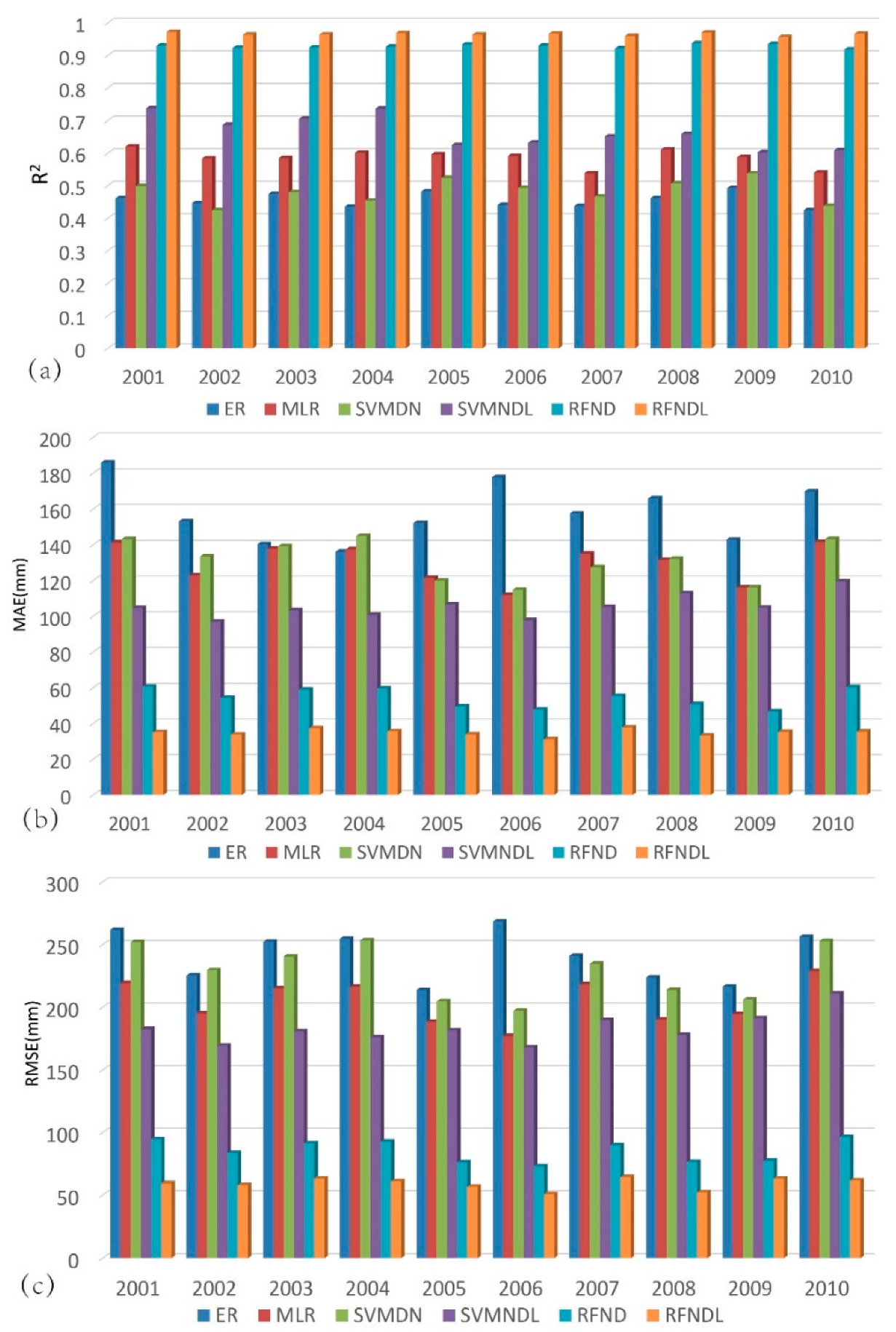
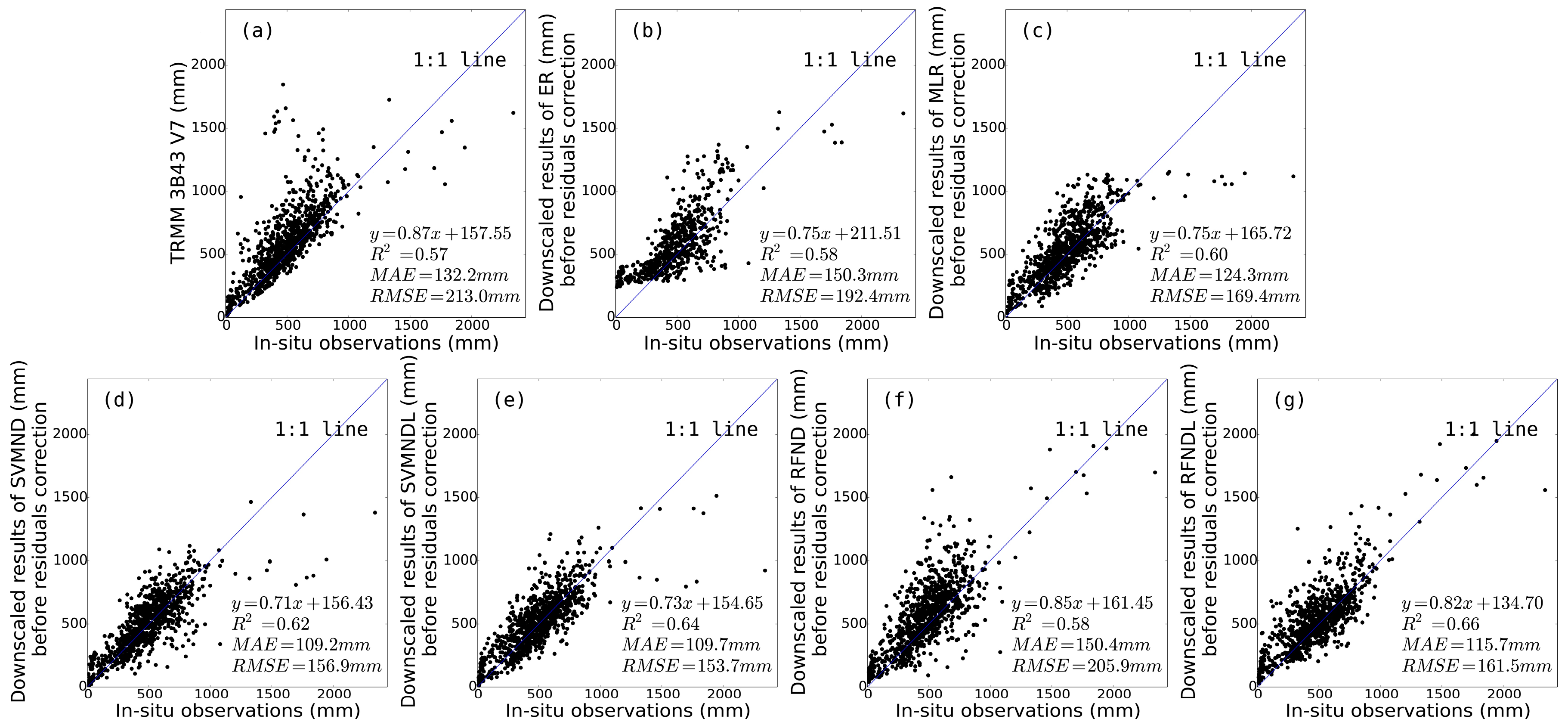
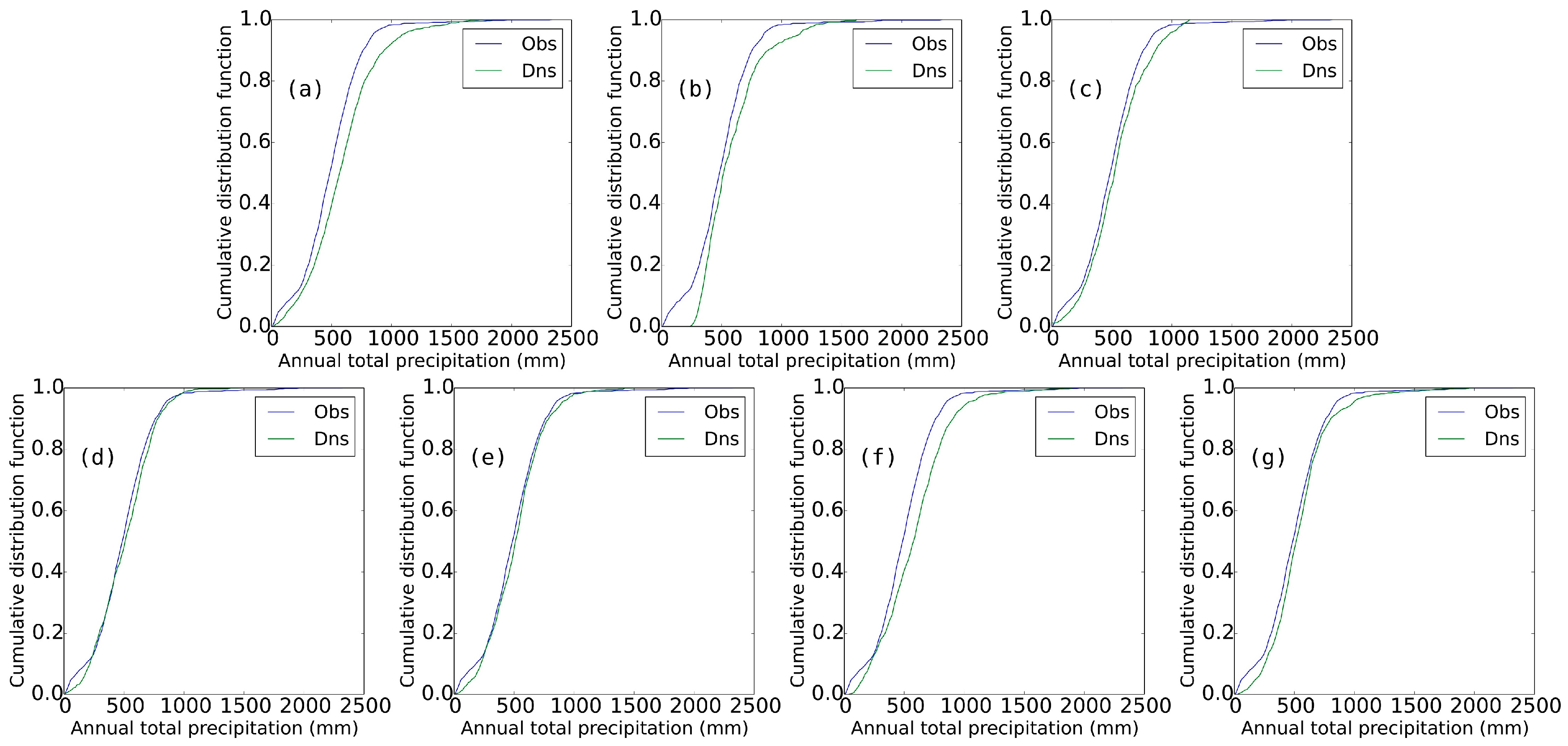
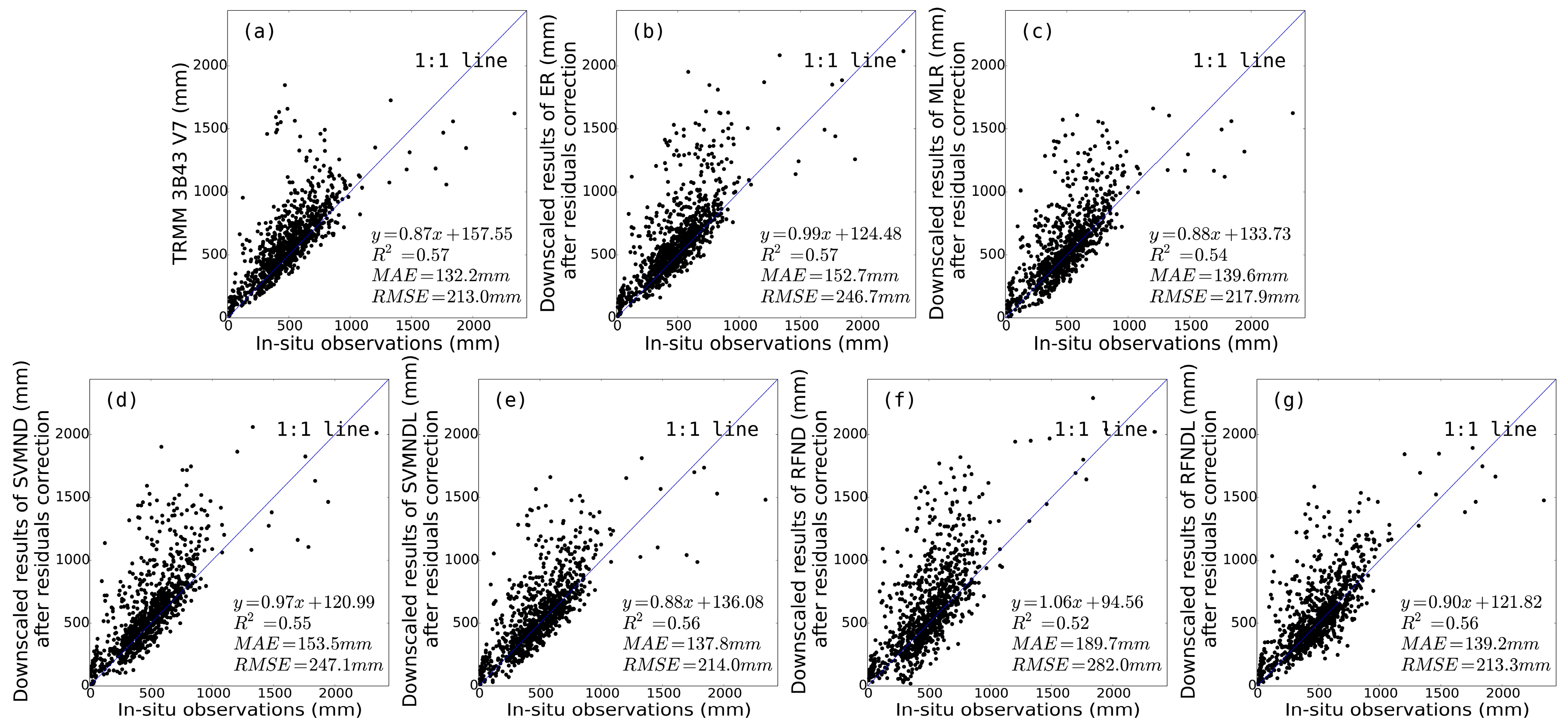
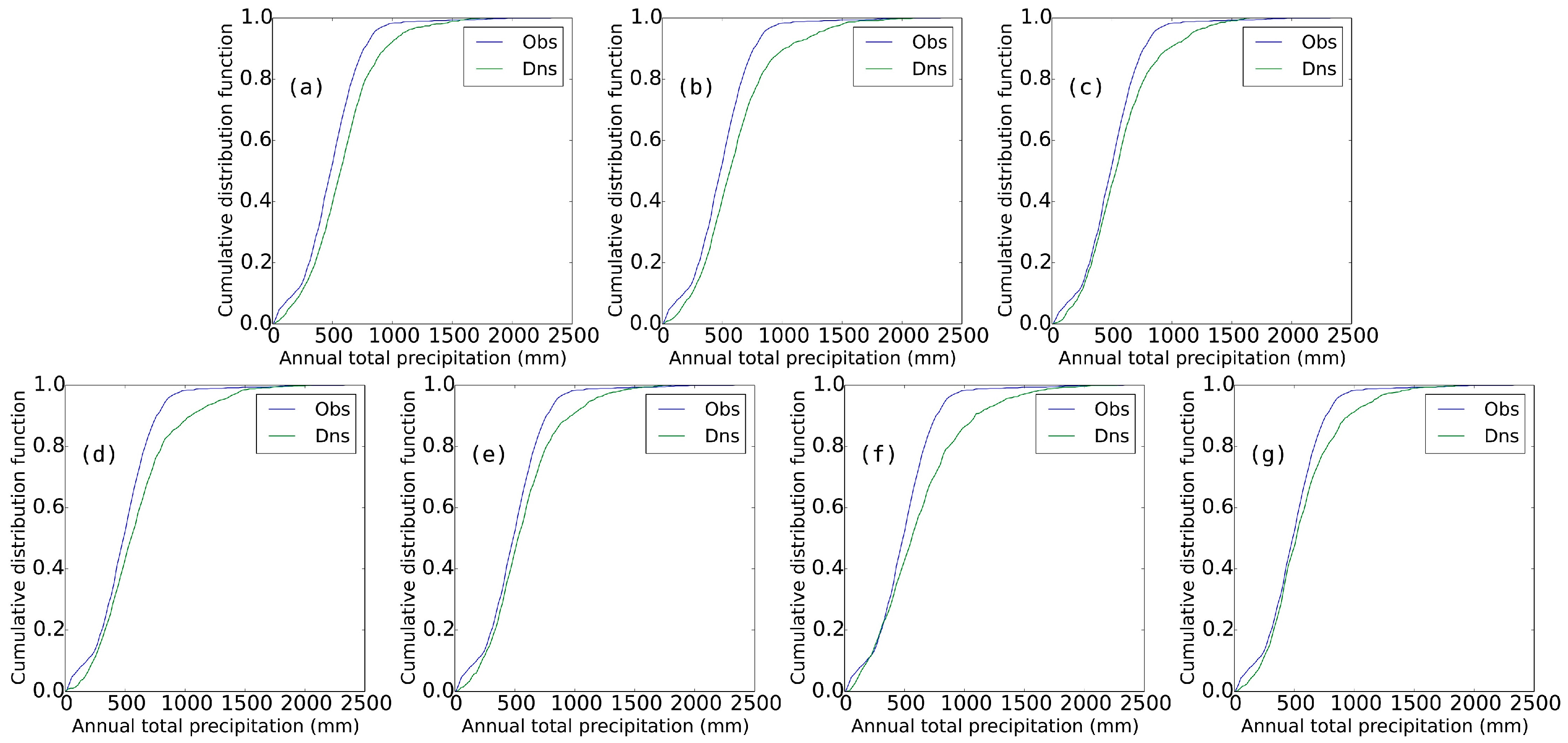
4.2.1. Validation with Rain Gauge Observations

The downscaled results of each algorithm were validated by using the observation records from 94 rain gauges over the Tibetan Plateau from 2001 to 2010, and were compared with the original TRMM 3B43 V7 data. The downscaled results before and after residual correction were all validated to assess the effects of residual correction. Figure 7a presents the scatter plot between TRMM 3B43 V7 and the observation records. Figure 7b–e shows the scatter plots between observation records and downscaled results of ER, MLR, SVMND, SVMNDL, RFND, and RFNDL before residual correction. Figure 8a–e shows the cumulative distribution function (CDF) of observations measured by stations compared with TRMM 3B43 V7 and downscaled results before residual correction derived from different algorithms. The original TRMM 3B43 V7 data was able to estimate the precipitation over the Tibetan Plateau with R² = 0.57, MAE = 132.2 mm and RMSE = 213 mm. The R² of the ER model increased marginally to 0.58; the MAE decreased to 150.3 mm; and the RMSE increased to 192.4 mm. The MLR model produced more accurate estimations than those of the ER and the original TRMM precipitation data with R² = 0.60, MAE = 124.3 mm and RMSE = 169.4 mm. RFNDL and SVMNDL estimated the similar accuracy with R² = 0.64 and 0.66, respectively, whereas MAE and RMSE of SVMNDL were marginally lower compared with RFNDL. However, the CDF comparison indicated that the downscaled results of SVM-based models showed minimum deviations from the CDF calculated from observations. Moreover, RFNDL exhibited worse results in capturing extreme precipitation (maximum and minimum) than SVM-based models.

For RF and SVM-based models, the performances of SVMNDL and RFNDL were better than those of SVMND and RFND, indicating that models including the combination of NDVI, DEM, and LSTs can provide more accurate downscaled results. Moreover, RFND produced much worse accuracy than SVMND. This indicates that the RF algorithm is more sensitive than SVM to LSTs when downscaling TRMM 3B43 V7 precipitation data over the Tibetan Plateau.

Figure 9a presents the scatter plot between TRMM 3B43 V7 and the observation records. Figure 9b–e shows the scatter plot between the observation records and downscaled results of ER, MLR, RFND, RFNDL, SVMND, and SVMNDL after residual correction. Compared with the downscaled results before residual correction, no obvious improvements of accuracy were produced by the residual correction. Figure 10a–e shows the cumulative distribution function (CDF) of observations measured by stations compared with TRMM 3B43 V7 and the downscaled results after residual correction derived from different algorithms. The CDFs of the downscaled results after residual correction presented greater deviation from the CDF calculated from observations than those before residual correction.

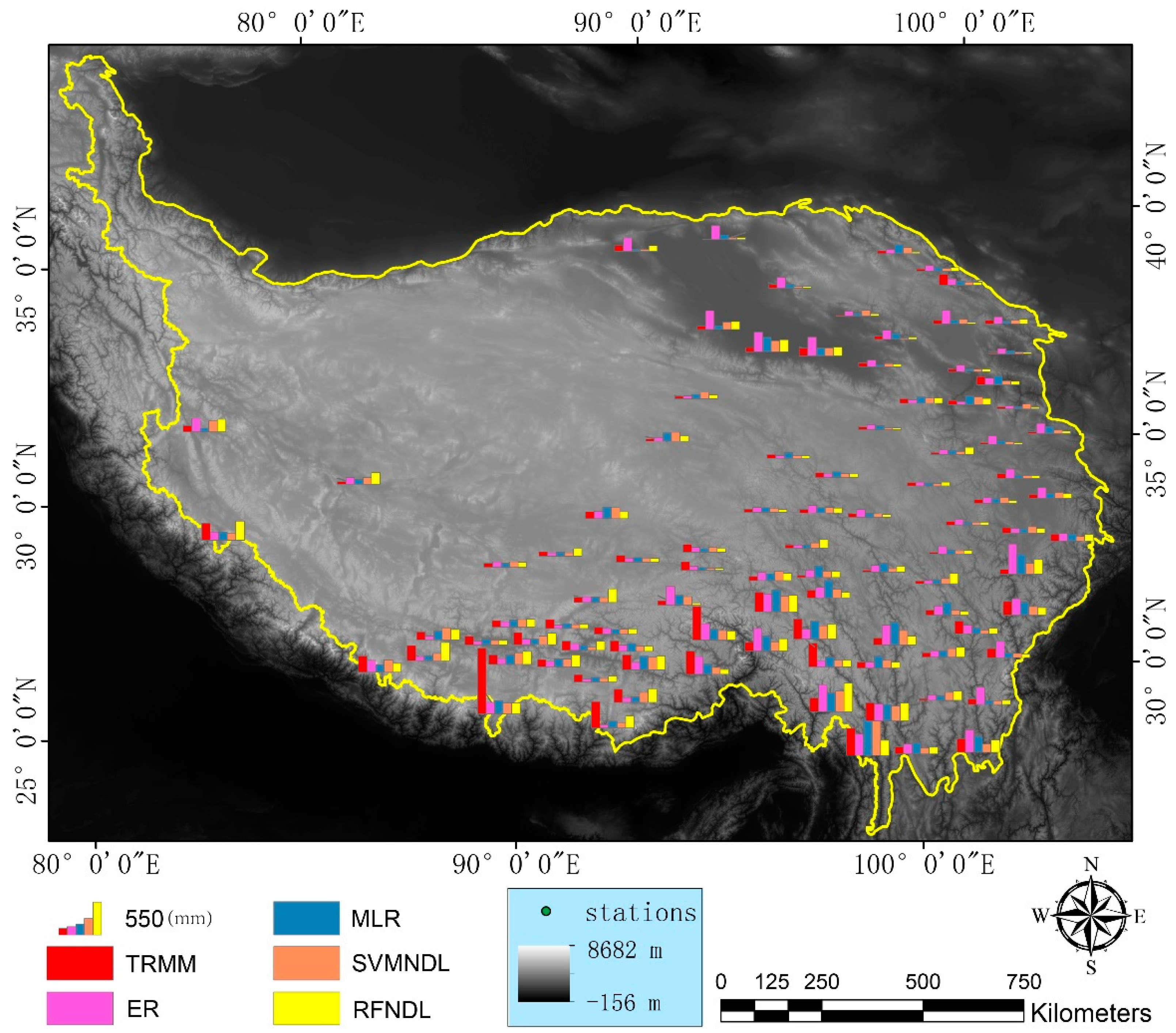
4.2.2. Spatial Distribution of Errors

To investigate the spatial distribution of the estimation errors, the MAE from 2001 to 2010 of the 93 rain gauges was calculated. Figure 11 presents the MAE of the original TRMM 3B43 V7 data and the downscaled results with ER, MLR, SVMNDL, and RFNDL before residual correction. In general, the MAEs tended to be higher in the southern part and lower over most others parts of the study area because the rainfall in that area is higher towards the south.

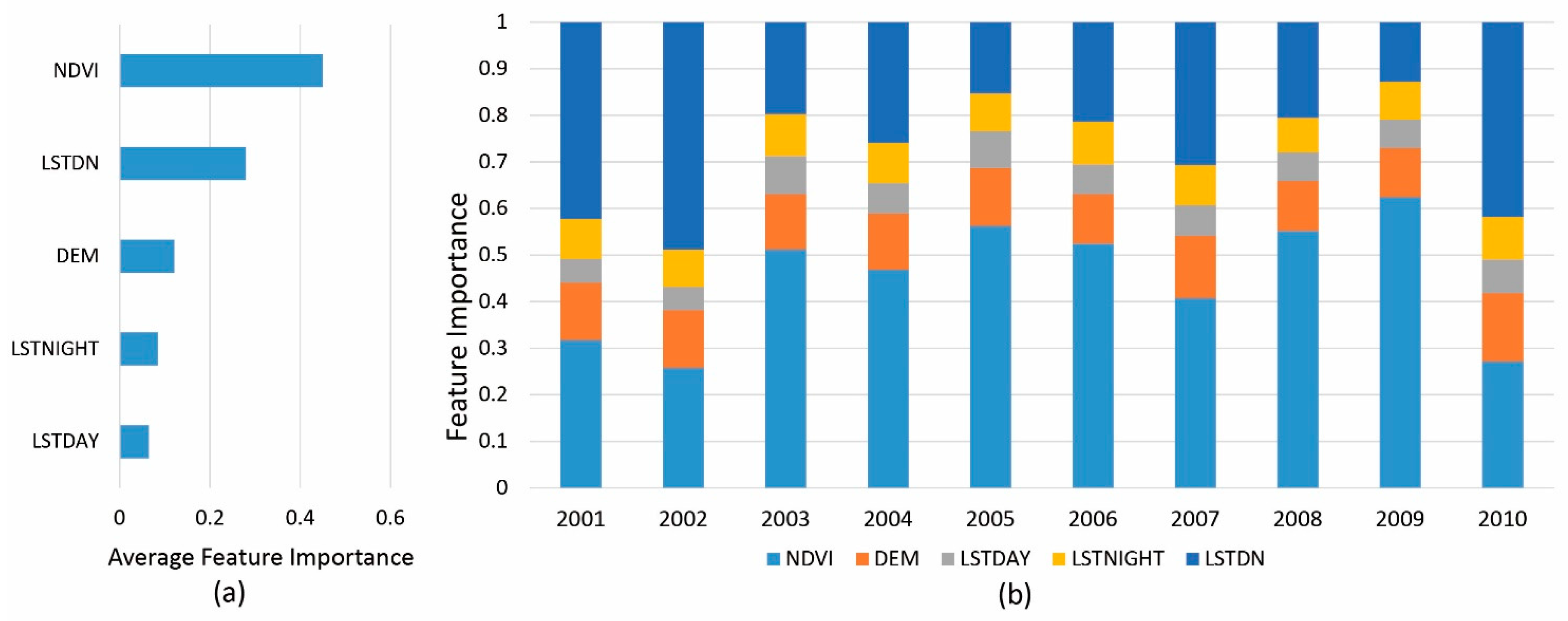
4.2.3. Variable Importance of the Random Forests Model

The RF algorithm provides measurements of variable importance. The resultant values are then used to rank the orderings of those independent variables in terms of their contribution to the regression model. The variable importance values were derived to quantify the usability of inclusion of land surface temperature features. Figure 12a shows the average variable importance of each variable from 2001 to 2010, termed as VI_NDVI, VI_DEM, VI_LSTDAY, VI_LSTNIGHT, and VI_LSTDN, and Figure 12b shows the importance of each variable for every individual year from 2001 to 2010. On average, VI_NDVI was the highest, followed by VI_LSTDN, VI_DEM, VI_LSTNIGHT, and VI_LSTDAY. This indicates that NDVI was the most significant variable when downscaling TRMM 3B43 V7 precipitation data over the Tibetan Plateau and that the day–night land surface temperature difference ranked second, highlighting the contribution of the land surface temperature feature to the downscaling model. Figure 12b shows that the VI_DEM, VI_LSTDAY, and VI_LSTNIGHT tended to be stable over each year and that VI_NDVI and VI_LSTDN were higher and more fluctuating than the other three independent variables.

5. Discussion

5.1. Value of Spatial Downscaling

Precipitation is the most active flux and greatest input to near surface hydrological system and thus strongly influences hydrological states and fluxes. Quantification of the spatial distribution of precipitation is thus significant to quantify these states and fluxes. Good estimates of the spatial variability of precipitation is especially crucial for accurate prediction of runoff response [36]. However, spatially continuous precipitation fields of fine resolution (e.g., 1 km) for regional hydrological and environmental studies are often not available, especially over sparsely gauged regions. Environmental monitoring of Earth from space has provided invaluable information for precipitation mapping. However, the use of satellite-based precipitation observations in hydrological and environmental applications is often limited by coarse spatial resolutions. Various downscaling models have been developed for mapping precipitation with fine resolution from satellite-based precipitation datasets [14,15,16,17,18,36,37,38]. In this study, we downscaled the annual total TRMM 3B43 V7 precipitation from the 25-km scale to 1-km spatial resolution over the Tibetan Plateau with integration of MODIS NDVI, LST, and DEM data using machine learning algorithms. Figure 13 shows a comparison of the TRMM precipitation of 2009 and the downscaled results using the RF model, zooming in on the mountainous (Figure 13d–e) and basin areas (Figure 13b,c) over the study region. It can be inferred from Figure 13 that the downscaled results at 1-km spatial resolution provide more detailed information and variations of the precipitation spatial distribution of the precipitation within each 25 km × 25 km grid cell. Precipitation data of fine spatial resolution can improve the characterization of the spatial variability of the precipitation and are useful for filling the gap between remotely-sensed spatial precipitation fields of low resolution and regional hydrologic and environment studies.

5.2. Usability of NDVI, DEM, and LST for Downscaling Precipitation Datasets

The response of vegetation to precipitation is widely acknowledged [39,40,41,42]. Moreover, vegetation type properties exert a strong influence on fluxes of sensible and latent heat into the atmosphere, directly affecting the humidity of the lower atmosphere and further influencing the development of moist convection, both locally and on atmospheric circulations on scales of tens to thousands of kilometers [2,5]. Thus, the precipitation–NDVI relationship is commonly used for downscaling the satellite-based precipitation dataset [14,15,18]. Figure 12 implies that the variable importance values of NDVI are higher than other variables. However, the precipitation–NDVI relationship is susceptible to several human and natural factors, which can limit the use of NDVI in downscaling satellite-based precipitation dataset over some regions [17]. For example, because almost no vegetation is present over barren regions such as deserts, precipitation has no influence on the NDVI over those regions.

The ability of DEM to downscale TRMM 3B43 has also been widely investigated over mountainous regions. Topography could influence the regional atmospheric circulation and the spatial pattern of precipitation through its thermal and dynamic forcing mechanisms [36,43]. In theory, the increase in elevation could increase the relative humidity of the air masses through expansion and cooling of the rising air masses, resulting in precipitation [44]. Therefore, the effect of topography on precipitation is much more direct and instantaneous over mountainous regions. However, the relationship is largely dependent on fluctuation of the terrain; precipitation tends to be unaffected by flat topography.

In this paper, we introduced land surface temperature as factors for downscaling TRMM 3B43 data. Co-variability of surface temperature and precipitation is observed globally [19]. As pointed out by Lemone et al. [45] and Trenberth et al. [19], if the ground is wet, more energy is likely to evaporate at the expense of sensible heating so that moisture acts as an “air conditioner.” Moreover, if the ground is wet from precipitation, the associated clouds likely block the sun, initially providing less energy and further reducing the temperature. In addition, high rates of evaporation could occur directly from bare soil after periods of rain, further suppressing sensible heat and surface temperature [20,46]. Thus the relationship of surface temperature–precipitation is more robust than those of NDVI–precipitation and topography–precipitation over sparsely vegetated regions such as deserts and barren land. In this study the land surface temperature in both daytime and nighttime were included for downscaling TRMM 3B43 V7 precipitation datasets. Moreover, the day–night temperature difference was calculated and included as an independent variable. The validation results demonstrate that models including LSTs produced higher accuracy. It can be inferred from Figure 12 that the variable importance values of LST_DN ranked second after the NDVI. Moreover, VI_DEM, VI_LSTDAY, and VI_LSTNIGHT tended to be stable over different years, and VI_NDVI and VI_LSTDN fluctuated more than the other three independent variables. This indicates that the contributions of DEM, LST_DAY, and LST_NIGHT to the RF model tend to be stable; the coupling relationship of precipitation–NDVI–LST_DN is more complicated and requires further research for improving the downscaling algorithm.

5.3. Residual Correction of Downscaled Results

Another issue that needs to be discussed is the fact that the downscaled results after residual correction showed worse accuracy than those before residual correction. In this study, we used a simple spline tension interpolator to interpolate the residual at coarse resolution to 1 km resolution. According to previous downscaling algorithms studies, the residual of the models represented the precipitation that could not be estimated by the models, and the spline tension interpolator [47] was widely used for acquiring interpolated residuals in previous downscaling models [14,15,17,18]. However, residual correction did not improve the accuracy of the downscaled results in this study. First, the residuals were interpolated only in two dimensions, without consideration of the errors resulting from topography; thus, incorporation of the impact of topography may be beneficial for improving the residual correction accuracy. Second, although the spline interpolation method is typically used for regularly spaced data, the performances of other interpolation algorithms (e.g., Kriging) need to be further evaluated. In addition, it is necessary to determine whether residual correction is necessary if the precipitation can be effectively predicted by the models and variables [17].

6. Conclusions

In this study, two machine learning algorithms, Random Forest (RF) and support vector machine (SVM), were used to downscale the yearly TRMM 3B43 V7 precipitation data from 25 km to 1 km. Moreover, daytime land surface temperature, nighttime land surface temperature, and day–night land surface temperature differences were introduced as new variables in addition to NDVI and DEM. A case study was conducted over the Tibetan Plateau area; downscaled results were validated based on the basis of meteorological stations and were compared with the algorithms proposed by Immerzeel et al. and Jia et al. [14,15].

The validation results showed that the RF and SVM-based models produced higher accuracy than the exponential regression (ER) and multiple linear regression (MLR) models. Furthermore, the RFNDL and SVMNDL showed better performance than the RFND and SVMND. When downscaling the precipitation only with NDVI and DEM, SVM performed much better than RF, indicating the significance of considering the relationship between land surface temperature and precipitation. The influence of the LSTs upon the accuracy of the RF model was greater than that for the SVM model.

According to the variable importance measurements of the RF, NDVI is the most significant variable, followed by LST_DN, DEM, LST_DAY, and LST_NIGHT. Moreover, the variable importance values of NDVI and LST_DN fluctuated more in different years than the other three independent variables. The downscaled results after residual correction showed worse accuracy than those before residual correction. Although residual correction may be unnecessary for the downscaled results when the precipitation could be effectively predicted by the models [17], the influence of different interpolation algorithms upon the results requires additional research and further examination.

In the future, other land surface features related to precipitation (such as soil moisture, slopes, and aspects) could be introduced to investigate whether these features are beneficial for downscaling satellite precipitation datasets. Moreover, further research will be undertaken to investigate algorithms for downscaling monthly or weekly precipitation datasets, which will hold great significance for hydrological, environmental, and ecological research.

References

1. Sapiano, M.R.P.; Arkin, P.A. An intercomparison and validation of high-resolution satellite precipitation estimates with 3-hourly gauge data. J. Hydrometeorol. 2009, 10, 149–166. [Google Scholar] [CrossRef]
2. Taylor, C.M.; de Jeu, R.A.M.; Guichard, F.; Harris, P.P.; Dorigo, W.A. Afternoon rain more likely over drier soils. Nature 2012, 489, 423–426. [Google Scholar] [CrossRef] [PubMed] [Green Version]
3. Goodrich, D.C.; Faurès, J.-M.; Woolhiser, D.A.; Lane, L.J.; Sorooshian, S. Measurement and analysis of small-scale convective storm rainfall variability. J. Hydrol. 1995, 173, 283–308. [Google Scholar] [CrossRef]
4. Ahmad, S.; Kalra, A.; Stephen, H. Estimating soil moisture using remote sensing data: A machine learning approach. Adv. Water Resour. 2010, 33, 69–80. [Google Scholar] [CrossRef]
5. Spracklen, D.V.; Arnold, S.R.; Taylor, C.M. Observations of increased tropical rainfall preceded by air passage over forests. Nature 2012, 489, 282–285. [Google Scholar] [CrossRef] [PubMed]
6. Song, Y.; Liu, H.; Wang, X.; Zhang, N.; Sun, J. Numerical simulation of the impact of urban non-uniformity on precipitation. Adv. Atmos. Sci. 2016, 33, 783–793. [Google Scholar] [CrossRef]
7. Xie, P.; Xiong, A.-Y. A conceptual model for constructing high-resolution gauge-satellite merged precipitation analyses. J. Geophys. Res. 2011. [Google Scholar] [CrossRef]
8. Morrissey, M.L.; Maliekal, J.A.; Greene, J.S.; Wang, J. The uncertainty of simple spatial averages using rain gauge networks. Water Resour. Res. 1995, 31, 2011–2017. [Google Scholar] [CrossRef]
9. Villarini, G.; Krajewski, W.F. Empirically-based modeling of spatial sampling uncertainties associated with rainfall measurements by rain gauges. Adv. Water Resour. 2008, 31, 1015–1023. [Google Scholar] [CrossRef]
10. Aghakouchak, A.; Mehran, A.; Norouzi, H.; Behrangi, A. Systematic and random error components in satellite precipitation data sets. Geophys. Res. Lett. 2012. [Google Scholar] [CrossRef]
11. Hsu, K.-L.; Gao, X.; Sorooshian, S.; Gupta, H.V. Precipitation estimation from remotely sensed information using artificial neural networks. J. Appl. Meteorol. 1997, 36, 1176–1190. [Google Scholar] [CrossRef]
12. Huffman, G.J.; Adler, R.F.; Arkin, P.; Chang, A.; Ferraro, R.; Gruber, A.; Janowiak, J.; Mcnab, A.; Rudolf, B.; Schneider, U. The global precipitation climatology project (GPCP) combined precipitation dataset. Bull. Am. Meteorol. Soc. 1997, 78, 5–20. [Google Scholar] [CrossRef]
13. Huffman, G.J.; Bolvin, D.T.; Nelkin, E.J.; Wolff, D.B.; Adler, R.F.; Gu, G.; Hong, Y.; Bowman, K.P.; Stocker, E.F. The TRMM multisatellite precipitation analysis (TMPA): Quasi-global, multiyear, combined-sensor precipitation estimates at fine scales. J. Hydrometeorol. 2007, 8, 38–55. [Google Scholar] [CrossRef]
14. Immerzeel, W.W.; Rutten, M.M.; Droogers, P. Spatial downscaling of TRMM precipitation using vegetative response on the Iberian Peninsula. Remote Sens. Environ. 2009, 113, 362–370. [Google Scholar] [CrossRef]
15. Jia, S.; Zhu, W.; Lű, A.; Yan, T. A statistical spatial downscaling algorithm of TRMM precipitation based on NDVI and DEM in the qaidam basin of china. Remote Sens. Environ. 2011, 115, 3069–3079. [Google Scholar] [CrossRef]
16. Chen, C.; Zhao, S.; Duan, Z.; Qin, Z. An improved spatial downscaling procedure for trmm 3b43 precipitation product using geographically weighted regression. IEEE J. Sel. Top. Appl. Earth Obs. Remote Sens. 2015, 8, 4592–4604. [Google Scholar] [CrossRef]
17. Xu, S.; Wu, C.; Wang, L.; Gonsamo, A.; Shen, Y.; Niu, Z. A new satellite-based monthly precipitation downscaling algorithm with non-stationary relationship between precipitation and land surface characteristics. Remote Sens. Environ. 2015, 162, 119–140. [Google Scholar] [CrossRef]
18. Shi, Y.; Song, L.; Xia, Z.; Lin, Y.; Myneni, R.; Choi, S.; Wang, L.; Ni, X.; Lao, C.; Yang, F. Mapping annual precipitation across mainland china in the period 2001–2010 from trmm 3b43 product using spatial downscaling approach. Remote Sens. 2015, 7, 5849–5878. [Google Scholar] [CrossRef]
19. Trenberth, K.E.; Shea, D.J. Relationships between precipitation and surface temperature. Geophys. Res. Lett. 2005. [Google Scholar] [CrossRef]
20. De Kauwe, M.G.; Taylor, C.M.; Harris, P.P.; Weedon, G.P.; Ellis, R.J. Quantifying land surface temperature variability for two sahelian mesoscale regions during the wet season. J. Hydrometeorol. 2013, 14, 1605–1619. [Google Scholar] [CrossRef]
21. Gislason, P.O.; Benediktsson, J.A.; Sveinsson, J.R. Random forests for land cover classification. Pattern Recognit. Lett. 2006, 27, 294–300. [Google Scholar] [CrossRef]
22. Shao, Y.; Lunetta, R.S. Comparison of support vector machine, neural network, and cart algorithms for the land-cover classification using limited training data points. ISPRS J. Photogramm. Remote Sens. 2012, 70, 78–87. [Google Scholar] [CrossRef]
23. Lary, D.J.; Alavi, A.H.; Gandomi, A.H.; Walker, A.L. Machine learning in geosciences and remote sensing. Geosci. Front. 2016, 7, 3–10. [Google Scholar] [CrossRef]
24. Zhang, Y.; Li, B.; Zheng, D. A discussion on the boundary and area of the Tibetan Plateau in China. Geogr. Res. 2002, 21, 1–8. [Google Scholar]
25. The National Meteorological Information Center. Available online: http://data.cma.cn/site/index.html (accessed on 11 August 2014).
26. The National Aeronautics and Space Administration (NASA) Precipitation Measurement Missions (PMM). Available online: http://pmm.nasa.gov/TRMM/trmm-instruments (accessed on 11 August 2014).
27. The NASA Land Processes Distributed Active Archive Center (LP DAAC). Available online: https://lpdaac.usgs.gov/ (accessed on 11 August 2014).
28. Jarvis, A.; Reuter, H.I.; Nelson, A.; Guevara, E. Hole-Filled SRTM for the Globe Version 4. Available online: http://Srtm.Csi.Cgiar.Org (accessed on 31 January 2016).
29. Pedregosa, F.; Varoquaux, G.; Gramfort, A.; Michel, V.; Thirion, B.; Grisel, O.; Blondel, M.; Prettenhofer, P.; Weiss, R.; Dubourg, V.; et al. Scikit-learn: Machine learning in python. J. Mach. Learn. Res. 2011, 12, 2825–2830. [Google Scholar]
30. Weng, Q. Remote sensing of impervious surfaces in the urban areas: Requirements, methods, and trends. Remote Sens. Environ. 2012, 117, 34–49. [Google Scholar] [CrossRef]
31. Mountrakis, G.; Im, J.; Ogole, C. Support vector machines in remote sensing: A review. ISPRS J. Photogramm. Remote Sens. 2011, 66, 247–259. [Google Scholar] [CrossRef]
32. Vapnik, V. The Nature of Statistical Learning Theory; Springer: New York, NY, USA, 1995. [Google Scholar]
33. Vapnik, V. Statistical Learning Theory; Wiley: New York, NY, USA, 1998. [Google Scholar]
34. Breiman, L. Random forests. Mach. Learn. 2001, 45, 5–32. [Google Scholar] [CrossRef]
35. Breiman, L.; Friedman, J.H.; Olshen, R.A.; Stone, C.J. Classification and Regression Trees; Chapman and Hall/CRC: Boca Raton, FL, USA, 1984. [Google Scholar]
36. Guan, H.; Wilson, J.L.; Xie, H. A cluster-optimizing regression-based approach for precipitation spatial downscaling in Mountainous Terrain. J. Hydrol. 2009, 375, 578–588. [Google Scholar] [CrossRef]
37. Xu, G.; Xu, X.; Liu, M.; Sun, A.; Wang, K. Spatial downscaling of TRMM precipitation product using a combined multifractal and regression approach: Demonstration for South China. Water 2015, 7, 3083–3102. [Google Scholar] [CrossRef]
38. Chen, F.; Liu, Y.; Liu, Q.; Li, X. Spatial downscaling of TRMM 3B43 precipitation considering spatial heterogeneity. Int. J. Remote Sens. 2014, 35, 3074–3093. [Google Scholar] [CrossRef]
39. Zhang, X.; Friedl, M.A.; Schaaf, C.B.; Strahler, A.H.; Liu, Z. Monitoring the response of vegetation phenology to precipitation in africa by coupling modis and trmm instruments. J. Geophys. Res. Atmos. 2005, 110. [Google Scholar] [CrossRef]
40. Wang, J.; Price, K.P.; Rich, P.M. Spatial patterns of NDVI in response to precipitation and temperature in the central great plains. Int. J. Remote Sens. 2001, 22, 3827–3844. [Google Scholar] [CrossRef]
41. Vicente-Serrano, S.M.; Gouveia, C.; Camarero, J.J.; Beguería, S.; Trigo, R.; López-Moreno, J.I.; Azorín-Molina, C.; Pasho, E.; Lorenzo-Lacruz, J.; Revuelto, J.; et al. Response of vegetation to drought time-scales across global land biomes. Proc. Natl. Acad. Sci. USA 2013, 110, 52–57. [Google Scholar] [CrossRef] [PubMed] [Green Version]
42. Zhong, L.; Ma, Y.; Salama, M.S.; Su, Z. Assessment of vegetation dynamics and their response to variations in precipitation and temperature in the Tibetan Plateau. Clim. Chang. 2010, 103, 519–535. [Google Scholar] [CrossRef]
43. Yin, Z.-Y.; Zhang, X.; Liu, X.; Colella, M.; Chen, X. An assessment of the biases of satellite rainfall estimates over the Tibetan Plateau and correction methods based on topographic analysis. J. Hydrometeorol. 2008, 9, 301–326. [Google Scholar] [CrossRef]
44. Sokol, Z.; Bližňák, V. Areal distribution and precipitation-altitude relationship of heavy short-term precipitation in the Czech Republic in the warm part of the year. Atmos. Res. 2009, 94, 652–662. [Google Scholar] [CrossRef]
45. Lemone, M.A.; Grossman, R.L.; Chen, F.; Ikeda, K.; Yates, D. Choosing the averaging interval for comparison of observed and modeled fluxes along aircraft transects over a heterogeneous surface. J. Hydrometeorol. 2003, 4, 179–195. [Google Scholar] [CrossRef]
46. Wallace, J.S.; Holwill, C.J. Soil evaporation from tiger-bush in South-West Niger. J. Hydrol. 1997, 188–189, 426–442. [Google Scholar] [CrossRef]
47. Franke, R. Smooth interpolation of scattered data by local thin plate splines. Comput. Math. Appl. 1982, 8, 273–281. [Google Scholar] [CrossRef]
Figure 1. The topography of the Tibetan Plateau and spatial distributions of the rain gauge stations.
Remotesensing 08 00655 g001
Figure 2. Flowchart of the downscaling algorithm used in this study.
Remotesensing 08 00655 g002
Figure 3. (a) Coefficients of determination (R2); (b) mean absolute error (MAE); and (c) root mean squared error (RMSE) of the simulated values using different algorithms compared with the original Tropical Rainfall Measuring Mission (TRMM) 3B43 V7 data from 2001 to 2010.
Remotesensing 08 00655 g003
Figure 4. (a) TRMM 3B43 V7 precipitation data and downscaled results before residual correction of (b) ER; (c) MLR; (d) SVMND; (e) SVMNDL; (f) RFND; (g) RFNDL in 2008.
Remotesensing 08 00655 g004
Figure 5. Interpolated residual of downscaling models in 2008: (a) ER; (b) MLR; (c) SVMND; (d) SVMNDL; (e) RFND; (f) RFNDL.
Remotesensing 08 00655 g005
Figure 6. (a) TRMM 3B43 V7 precipitation data and downscaled results after residual correction of (b) ER; (c) MLR; (d) SVMND; (e) SVMNDL; (f) RFND; (g) RFNDL in 2008.
Remotesensing 08 00655 g006
Figure 7. Scatter plot between the observations and (a) TRMM 3B43 V7 precipitation data and downscaled results before residual correction using (b) ER; (c) MLR; (d) SVMND; (e) SVMNDL; (f) RFND; and (g) RFNDL of 2001–2010.
Remotesensing 08 00655 g007
Figure 8. Cumulative distribution function (CDF) of the observations and (a) TRMM 3B43 V7 precipitation data and downscaled results before residual correction using (b) ER; (c) MLR; (d) SVMND; (e) SVMNDL; (f) RFND; and (g) RFNDL of 2001–2010.
Remotesensing 08 00655 g008
Figure 9. Scatter plot between the observations and (a) TRMM 3B43 V7 precipitation data and downscaled results after residual correction using (b) ER; (c) MLR; (d) SVMND; (e) SVMNDL; (f) RFND; and (g) RFNDL of 2001–2010.
Remotesensing 08 00655 g009
Figure 10. Cumulative distribution function (CDF) of the observations and (a) TRMM 3B43 V7 precipitation data and downscaled results after residual correction using (b) ER; (c) MLR; (d) SVMND; (e) SVMNDL; (f) RFND; and (g) RFNDL of 2001–2010.
Remotesensing 08 00655 g010
Figure 11. Spatial distribution of mean absolute error (MAE) of original TRMM 3B43 V7 data and downscaled results before residual correction using ER, MLR, SVMNDL, and RFNDL compared to observations.
Remotesensing 08 00655 g011
Figure 12. (a) Average variable importance from 2001 to 2010; (b) variable importance of each year.
Remotesensing 08 00655 g012
Figure 13. (a) Elevation of the Tibetan Plateau and the indictor boxes for basin area and mountainous area; (b) TRMM 3B43 annual total precipitation map of the basin area of 2009; (c) downscaled annual total precipitation map of the basin area of 2009; (d) TRMM 3B43 annual total precipitation map of the mountainous area of 2009; (e) downscaled annual total precipitation map of the mountainous area of 2009.
Remotesensing 08 00655 g013