Improving Land Use/Cover Classification with a Multiple Classifier System Using AdaBoost Integration Technique


1
School of Geography and Planning, Sun Yat-sen University, No. 135 Xinggangxi Road, Guangzhou 510275, China
2
Department of Geography, Florida State University, Tallahassee, FL 32306-2190, USA
*
Author to whom correspondence should be addressed.
Remote Sens. 2017, 9(10), 1055; https://0-doi-org.brum.beds.ac.uk/10.3390/rs9101055
Submission received: 19 August 2017
/
Revised: 21 September 2017
/
Accepted: 10 October 2017
/
Published: 17 October 2017
Abstract
:Guangzhou has experienced a rapid urbanization since 1978 when China initiated the economic reform, resulting in significant land use/cover changes (LUC). To produce a time series of accurate LUC dataset that can be used to study urbanization and its impacts, Landsat imagery was used to map LUC changes in Guangzhou from 1987 to 2015 at a three-year interval using a multiple classifier system (MCS). The system was based on a weighted vector to combine base classifiers of different classification algorithms, and was improved using the AdaBoost technique. The new classification method used support vector machines (SVM), C4.5 decision tree, and neural networks (ANN) as the training algorithms of the base classifiers, and produced higher overall classification accuracy (88.12%) and Kappa coefficient (0.87) than each base classifier did. The results of the experiment showed that, based on the accuracy improvement of each class, the overall accuracy was improved effectively, which combined advantages from each base classifier. The new method is of high robustness and low risk of overfitting, and is reliable and accurate, and could be used for analyzing urbanization processes and its impacts.
1. Introduction
Land use/cover (LUC) has been changed drastically due to urbanization in the past decades [1,2], and more built area has appeared to provide space for development. Such changes also caused a series of negative effects on human society, such as increasing flood risk [3], deteriorating environment [4], degrading ecosystem [5], and so on. To better understand these impacts, LUC changes (LUCC) caused by urbanization need to be quantified accurately. Remote sensing is the latest technique that has been used to estimate LUCC [6,7,8,9], and the Landsat imagery acquired by MSS, TM, ETM+ and OLI sensors have been widely used for such a purpose [10] due to its long records and free availability [11,12].
Quantitative LUCC estimation has mainly been driven from remotely sensed imagery using various classification algorithms [13,14], which can be divided into supervised algorithms and unsupervised algorithm [15]. Decision trees, support vector machines (SVM), artificial neural networks (ANN) and maximum likelihood classifier are supervised classification algorithms [16,17,18], and K-means algorithm, fuzzy c-means algorithm and AP cluster algorithm are typical unsupervised classification algorithms [19,20,21,22]. These algorithms have been widely used in estimating LUCC with satellite remote sensing. For example, Pal and Mather [23] used SVM to classify land cover with Landsat ETM+ images, and Tong et al. [24] detected urban land changes of Shanghai in 1990, 2000 and 2006 by using artificial backpropagation neural network (BPN) with Landsat TM images.
Different classification algorithms have been found to have different advantages in classifying different LUC categories; however, none could produce perfect classification accuracy to all LUC categories [25,26]. One classification algorithm may have pretty good performance to a specific LUC category, but may have some disadvantages on other LUC categories [27]. For example, SVM with RBF (radial basis function) kernel has been found could have an accuracy of 95% to grassland, but only have a low accuracy of 60.3% to houses [28]; maximum likelihood classifier performed better for bare soil with a high accuracy (98.01%), but not for built-up area with only a much lower accuracy (75%) [26]; and, with k-NN (k-Nearest Neighbor), the classification accuracy of continuous urban fabric reached 97%, but that for cultivated soil was only 49% [29].
There is requirement for higher classifying accuracy in studying the impact of LUC changes on flooding, particularly in large scale watershed [30]. Multiple classifier systems (MCS) are a newly emerged classification algorithm that combines the classification results from several different classification algorithms. The purpose of MCS is to achieve a better classification result than that acquired by using only one classifier [31,32,33,34,35,36]. MCSs can be divided into two categories according to specific methods for combining the classification results. The first one is called multiple algorithm MCS, and the final result is generated by combining the classification results from a group of specific classifiers as base or component classifiers with identical training samples. The second one is called as single algorithm MCS, and the final result is generated from a single base algorithm. The core of MCS is to combine the results provided by different base classifiers, and the earliest method for combination was through the majority voting. By now, some more approaches have been proposed for classifier combination, such as Bayes approach, Dempster-Shafer theory, fuzzy integral, and so on [37,38,39,40]. Previous studies have shown that MCS are effective for LUC classification. For example, Dai and Liu [41] constructed a MCS with six base classifiers, i.e., maximum likelihood classifier (ML), support vector machines (SVM), artificial neural networks (ANN), spectral angle mapper (SAM), minimum distance classifier (MD) and decision tree classifier (DTC), and the classifier combination was through voting strategy. Their results showed that MCS obtained higher accuracy than those achieved by its base classifiers. Zhao and Song [42] proposed a weighted multiple classifiers fusion method to classify TM images, and their results showed that a higher classification accuracy has been achieved by MCS. Based on different guiding rules of GNN (granular neural networks), Kumar and Meher [43] proposed an efficient MCS framework with improved performance for LUC classification.
For an improved performance, a base classifier to be included in a multiple classifier system (MCS) should be more accurate in at least one category than other classifiers, suggesting that base classifiers should be selected from diverse families of pattern recognizers [44]. For a MCS using different classifiers, the diversity is measured by the difference among the base classifier’s pattern recognition algorithms [45]. We generally prefer to combine the advantages of different algorithms based on priori-knowledge. However, there is a need to train a few different classification algorithms, and they could be easily over-fitted without sufficient priori-knowledge [34,46,47,48,49]. Moreover, because the algorithms currently developed for land use/cover classification are relatively limited, the diversity of MCS can be low, which can further affect its performance. For a MCS based on one classification algorithm, classification accuracy can be improved by combining many diverse classifiers [50,51], which can be easily produced with plenty of sample sets. Disadvantage of this type of MCS is that the base classifiers are based on one classification algorithm, the difference among various classification algorithms is not considered.
Popular MCS combination techniques include Bagging, Boosting, random forests, and AdaBoost with iterative and convergent nature [46,52,53,54,55,56]. To obtain more base classifiers with differences, Ghimire and Rogan [54] performed land use/cover classification in a heterogeneous landscape in Massachusetts by comparing three combining techniques, i.e., bagging, boosting, and random, with decision tree algorithm, and their results showed that the MCS performed better than the decision tree classifier. Based on SVM, Khosravi and Beigi [55] used bagging and AdaBoost to combine a MCS to classify a hyperspectral dataset, and their work has showed a high capability of MCS in classifying high dimensionality data.
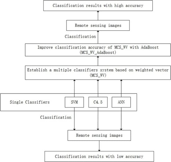
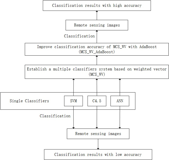
In this paper, a method was proposed, which can help improve the combination for multiple classifiers systems and thus increase land use/cover classification accuracy. It is called as MCS_WV_AdaBoost, which can combine the advantages of the multiple classifier systems based on a single classification algorithm and on multiple algorithms. In this method, a MCS based on weighted vector combination (called as MCS_WV) was established, which can combine decisions of component classifiers trained by different algorithms, and then the AdaBoost method was employed to boost the classification accuracy of MCS_WV (MCS_WV improved by AdaBoost, called as MCS_WV_AdaBoost). MCS_WV_AdaBoost inherits the benefits of MCS_WV which combines the advantages from different classification algorithms and reduces overfitting, resulting in more stable classification performance. In addition, MCS_WV_AdaBoost exhibits more component classifiers with diversity, resulting in larger improvement in classification accuracy. The proposed method was further used to produce a time series of land cover maps from Landsat images for a highly dynamic, large metropolitan area. The proposed method was found to be effective and can help improve land use/cover classification results.
2. Study Area and Data
2.1. Study Area
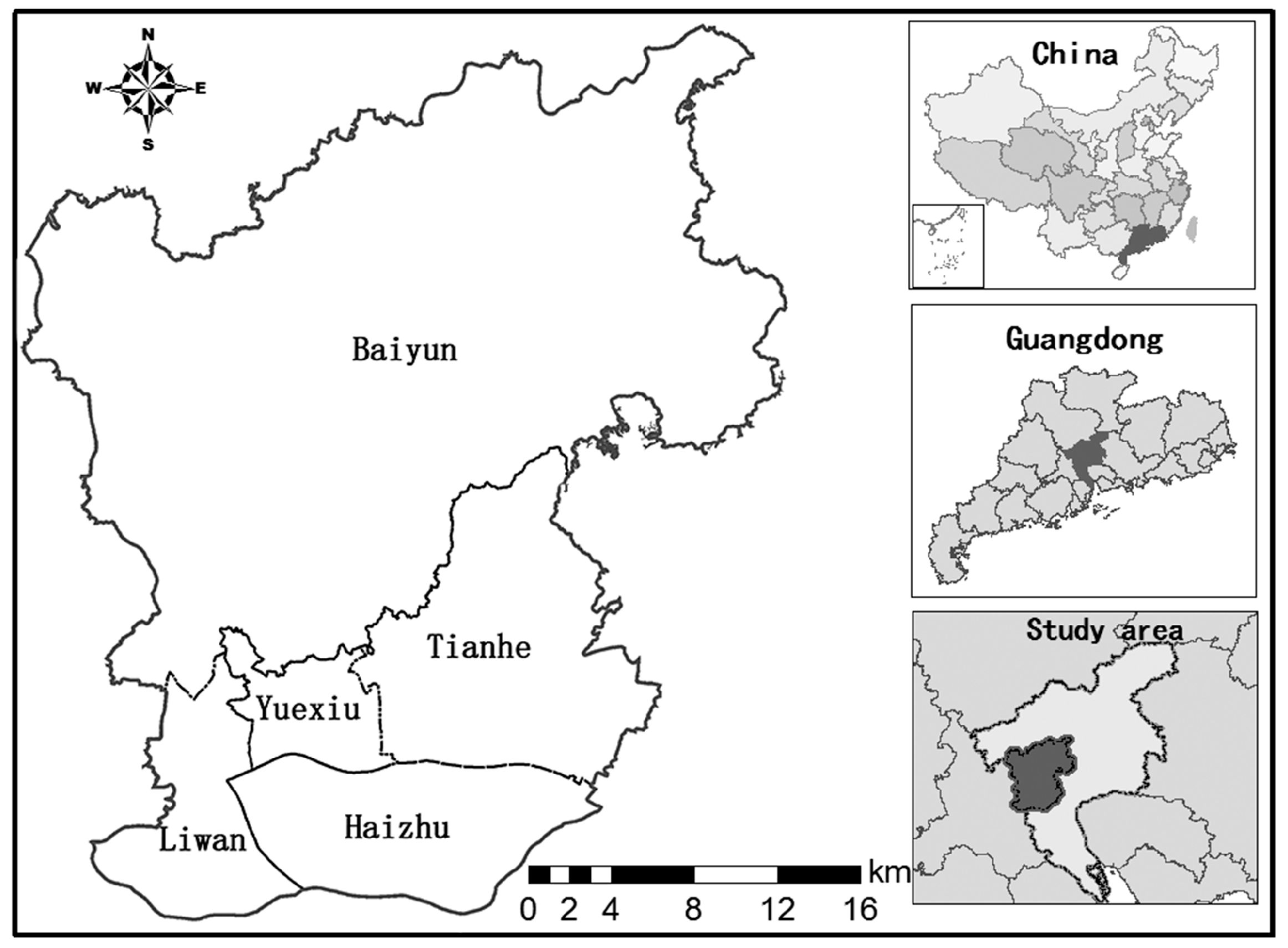
Guangzhou, the capital city of Guangdong province in southern China, is located at the confluence of East River, West River and North River. It is not only the political, economic and cultural center of Guangdong province, but also the most densely populated region in the province. Guangzhou has been a forerunning city since 1978 when China opened its door to the western world and initiated its economic transformation. Guangzhou has experienced dramatic economic development and rapid urbanization, which have prompted dramatic changes in land use/cover. Therefore, it is of great importance to develop a robust and good classification scheme to map the LUC in this region. The study area covers the major urban area of Guangzhou City, including five districts, namely, Liwan, Yuexiu, Haizhu, Tianhe and Baiyun, with a total area of 7434.4 km2 (Figure 1).
2.2. Data and Pre-Processing
The primary data used in this study are a time series of cloud-free Landsat images with WRS Path 121 and Row 44 acquired by Landsat-5 Thematic Mapper (TM), Landsat-7 ETM+ (Enhanced Thematic Mapper Plus) and Landsat-8 Operational Land Imager (OLI) sensors. We used images from different time periods, mainly to prove the generalization of the proposed method. All images were acquired from US Geological Survey (USGS) EROS Data Center. All images were acquired during a dry season including the months of January, February, November and December when clouds are scarce and surface features rarely change. The thermal band (Band 6) of Landsat TM and ETM+ contains little information of surface radiation that is not quite valuable for land use/cover classification. Thus, only Bands 1–5 and Band 7 of TM and ETM+ were actually used in this study. Landsat-8 OLI has nine bands including all ETM+ bands, and, to avoid atmospheric absorption, only Bands 2–7 were used. In total, 11 Landsat images from 1987 to 2015 were acquired, with an interval of 2–4 years. Table 1 provides brief information on the Landsat images used in this study. The FLAASH model in ENVI was used for the atmospheric correction of Landsat images for more clearly features recognizing. The selected images were geometrically registered to an aerial photograph with Universal Transverse Mercator (UTM) projection (zone 49 N), and the geometric error was less than 1 pixel (30 m). Then, the images were clipped by a mask of the study area.
3. Methods
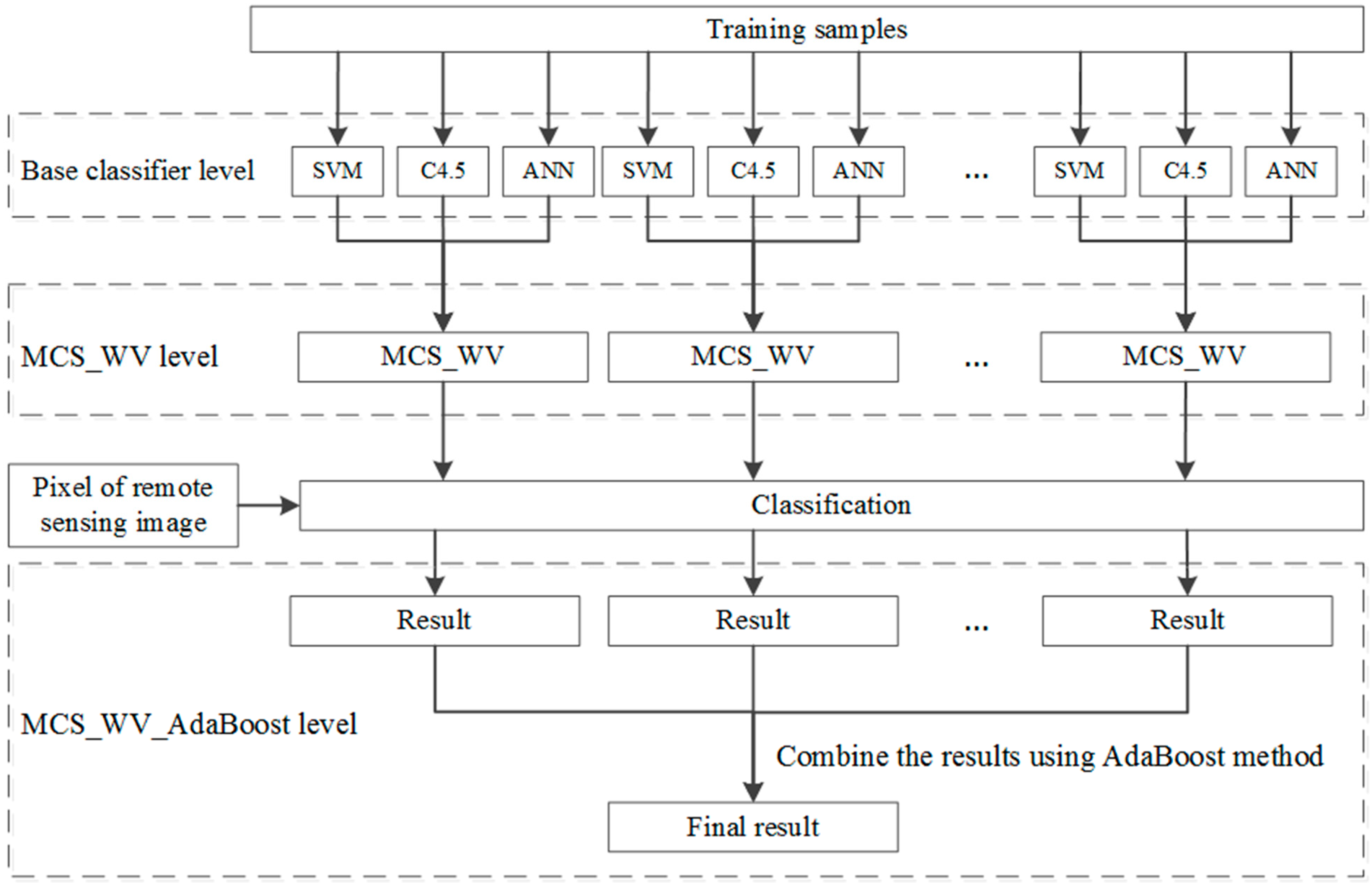
Figure 2 illustrates the classification method of this study. The process can be divided into three levels. The first level is called “Base classifier level”, providing the base classifiers using different classification algorithms. The second level is called “MCS_WV level”, which produces many MCS_WVs with AdaBoost iterative and convergent nature. MCS_WV is a composed classifier combining the base classifier’s decision with a weight vector. The third level is “MCS_WV_AdaBoost level”. At this level, the classification results of MCS_WVs are combined with AdaBoost method and a more accurate classification is produced.
3.1. Training Algorithms for Base Classifiers
Utilizing the advantage of each base classifier to improve the classification accuracy is the core of MCS [56]. For better combination, the algorithms for base classifier training should be complementary to each other [57,58,59]. Support vector machine (SVM), C4.5 decision tree and artificial neural network (ANN) are among the most used remote sensing image classification algorithms, and are also quite different in land cover classification, thus have diversities [59,60,61,62,63]. For this reason, they are selected as the base classifiers here.
3.1.1. Support Vector Machine
Support Vector Machine (SVM) is a machine learning method proposed by Vapnik in the 1990s [62]. The training data were mapped to a higher dimension to find an optimal hyperplane to separate the tuples tagged the same class from others. The algorithm is quite robust and would not be affected by adding or removing samples for support vectors. It can generate high accuracy for modeling complex nonlinear decision boundaries and is not easy to be over fitting. In fact, it is one of the most ideal algorithms for remote sensing classification [63].
3.1.2. C4.5 Decision Tree
C4.5 is a decision tree proposed by Quinlan based on the ID3 algorithm. In this algorithm, the decision tree is built by dividing the sample set layer-by-layer, where the split property is the one which has the highest information gain ratio with the sample set and the optimal threshold under the split property obtained by information entropy calculating [64]. C4.5 decision tree has advantages of strong logicality, its rules are simple and easy to be understood, and thus is perfect for noise suppressing. It is suitable for more complex multi-source or multi-scale data, and is also an excellent classifier for remote sensing image classification.
3.1.3. Artificial Neural Network
Artificial neural networks ANN is an algorithm that simulates the function of human brain based on a neural network composed by an input layer, hidden layers and an output layer [65]. Its best-known architecture, namely back-propagation artificial neural network (BPANN), was used for classification in this study. Through the input layer, sample information forwards propagation and the errors back propagation, the weights of path between neurons in different layers are adjusted constantly to determine which class the input sample possibly should be, until the error of the output of the network is small enough or the times of learning reaching its upper limit [66]. It is a strong adaptive and self-learning algorithm that can consider many kinds of factors and uncertain information. ANN can adapt to the rich texture and high spectrum confusion of remote sensing, especially by setting the nodes in hidden layers, the problem of “homogeneous spectrum” and “foreign matter” can be solved perfectly in the process of remote sensing classification [67].
3.2. Multiple Classifiers System Based on Weight Vector and Its Improved Version Using AdaBoost
3.2.1. Multiple Classifiers System Based on Weight Vector
The sensitivities of classifiers vary by classes. The difference between base classifiers is critical to build a multiple classifiers system [68]. In this paper, the sensitivity of each base classifier with respect to different classes is represented by weight vectors. Firstly, the training samples (the samples with known labels) are grouped into the training and validation parts and then assume M as a base classifier set, M = {M1, M2, M3, …, MK}, K is the count of base classifiers; X as the sample set, X = {X1, X2, X3, …, XN}, N is the count of samples sets; Ω as classes set, Ω = {ω1, ω2, ω3, …, ωC}, C is the total number of classes. Then, suppose the weight vector of classifier Mi (i = 1, 2, 3, …, K) is Wi, tij is the count of the validation samples which were classified as class ωj by classifier Mi, eij reflects the count of samples error recognized as class ωj by classifier Mi, the weight classifier Mi to class ωj , Wij , can be expressed as Equation (1):
Thus, the weight vector of classifier Mi voting for the class of validation samples is
Finally, the classification result of an instance x can be calculated via weighted voting with Equation (4):
where M(x) means x is classified by Mi.
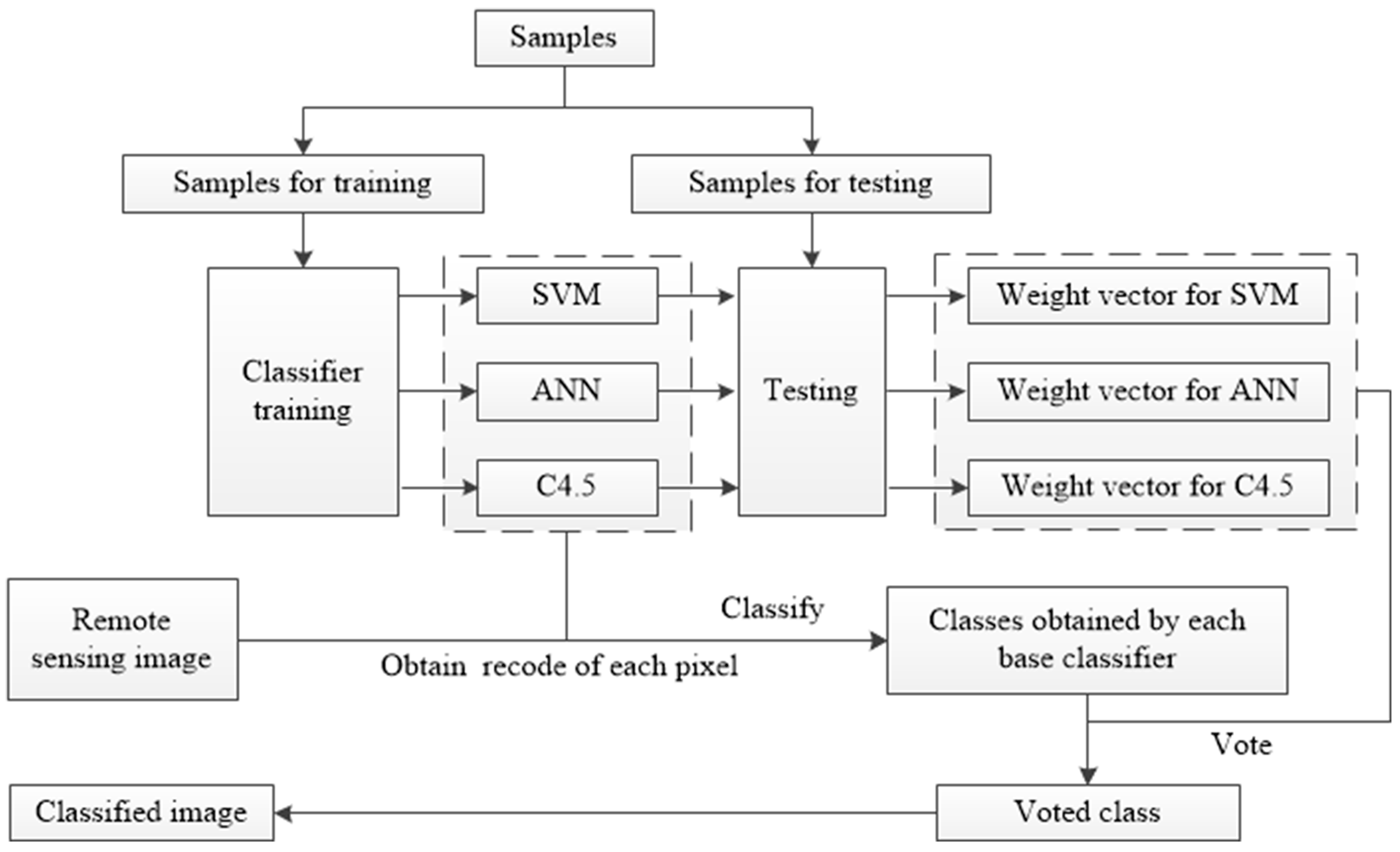
Figure 3 illustrates the flow chart of the MCS_WV classification. First, the samples were divided into two parts with one part as the training subset and the other part as the validation subset. For each pixel in each base, the classifier generated a classification, and, using the weight vector of each base classifier, the final class label was determined by weighted voting.
3.2.2. AdaBoost
AdaBoost (Adaptive Boosting) is an algorithm which can be used to boost the performance of a classification algorithm [69,70]. First, entrusts with the same weight to each sample, and then train a new classifier with the sample set which obtained by using the method of sampling with replacement. Classify the samples in the set, and give higher weight to the misclassified samples and lower weight to the correctly classified ones. The weight decides the chance of being used to train classifier in the next iteration. Thus, the new classifier focuses more on the misclassified samples in the previous iteration. More than one classifiers are trained with the sample sets obtained from the reweighed samples [71,72]. After all iterations, the final hypothetic class is calculated using weighted voting.
3.2.3. Multiple Classifiers System Based on Weight Vector Improved by AdaBoost
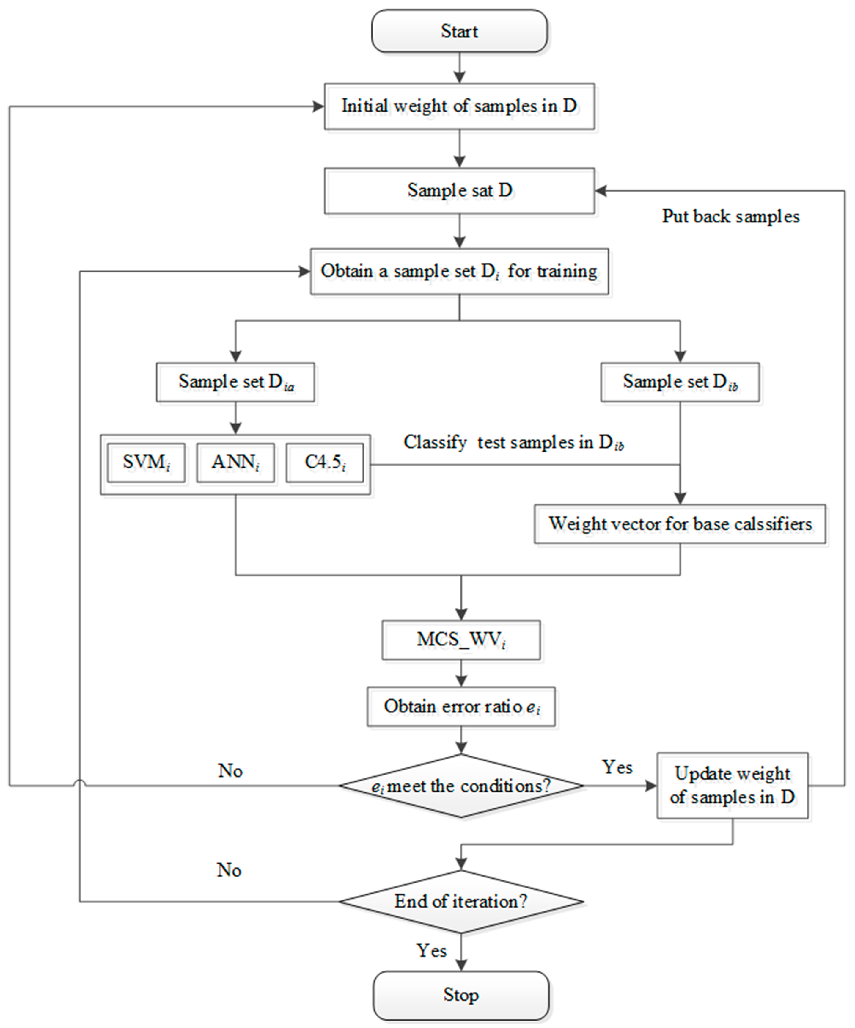
The MCS_WV has strong relationship with the priori knowledge, and its performance may be limited if the validation sample set is inadequately representative. To make MCS_WV classification model stable with high accuracy, AdaBoost algorithm is used to help improve the performance. As shown in Figure 4, first, initial the weights of samples in sample set D, and then extract a sample set Di by sampling with replacement. Di was divided into two parts: Dia for base classifier (SVMi, ANNi, and C4.5i) training, and Dib for creating weight vectors. With the base classifier and weight vectors, a composite classifier MCS_WVi was generated. The error ratio is calculated by classifying the samples in D, and the misclassified samples are given higher weight for next iteration. In each iteration, the weight of each sample is adjusted to make MCS_WV classifiers focus on the hard classified samples until the end. Finally, a classifier set of MCS_WV is produced, and the category of pixels of RS image can be diagnosed by MCS_WV classifiers which improved by AdaBoost algorithm (MCS_WV_AdaBoost).
3.3. Base Classifier Contribution Calculate Method
In this study, we used the weight of each single classifier to calculate its contribution in classification. The contribution can be calculated using Equations (5) and (6):
where, i and j denote a sample and classifier, respectively; n is the total number of samples; m is number of classifiers; Cij is contribution of classifier j to decide sample i; wij is the weight of classifier j to classify i; and Cj indicates the contribution of classifier j in classification.
4. Results
4.1. Train Sample Selection
To analyze land use/cover distribution in Guangzhou, six LUC types were identified, including forest (FO), grassland (GR), bare land (BL), built-up area (BA), cultivated land (CL) and waters (WA). Because the combination of bands 3–5 of TM/ETM+ or bands 3, 5 and 6 of OLI has a better visual effect, an image interpretation key for various land use/cover types was established for sample selection.
In this study, samples were categorized into reference sample set and training sample set. A grid with resolution of 5 km was used to control the distribution of training samples. For each LUC class, about 200 pure pixels distributed uniformly in the grid cells that contain the current LUC type were selected for classifier training. The number of samples contained in each class in the training sets is shown in Table 2. In each grid cell, about 50 points were generated randomly, and then labeled each point with LUC type using the Landsat image. Finally, 2135 points were used as the reference to verify the classification performance.
4.2. Classification and Accuracy Analysis
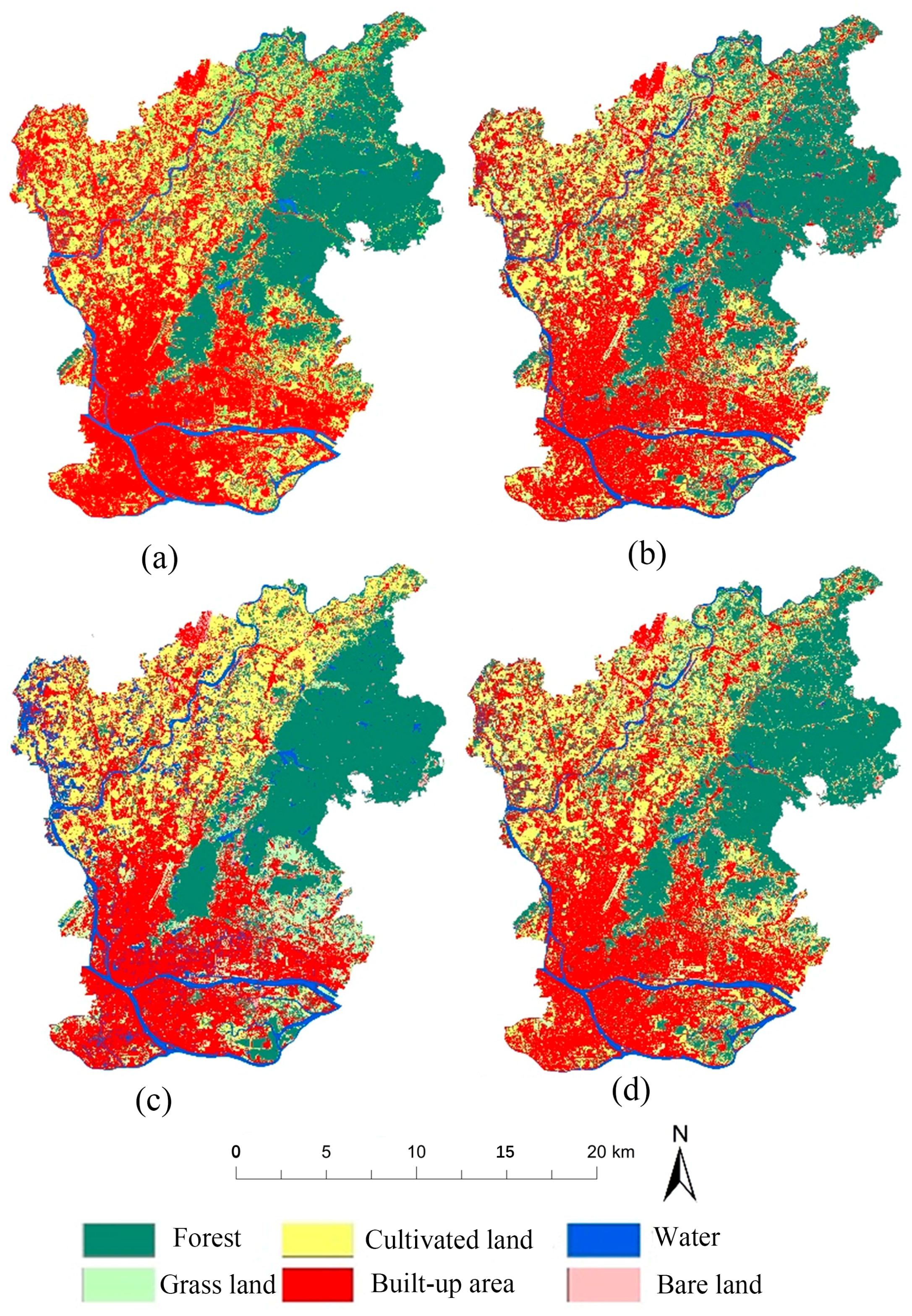
Using SVM (RBF is used as the kernel function), ANN (it is composed of one input layer, one hidden layer, and one output layer) and C4.5 (the tree height is 7), 11 land use/cover maps were generated from Landsat images spanning the period of 1987 to 2015 (see Table 1). The MCS_WV_AdaBoost algorithm proposed here was used to help improve classification accuracy. Figure 5 illustrates the classification results for 2001 that were generated by the three classifiers.
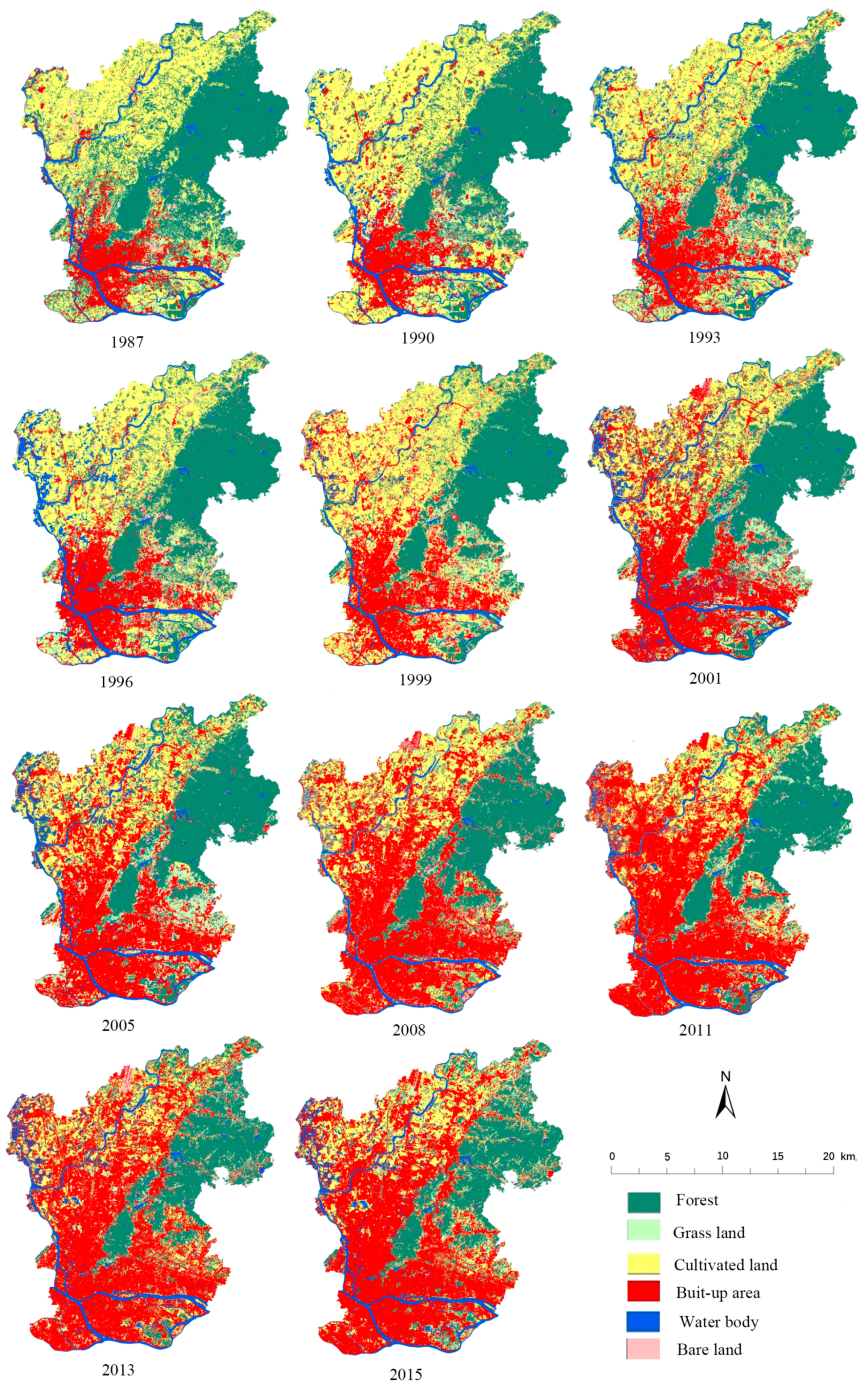
Thematic mapping accuracy by each classifier was assessed, as summarized in Table 3. SVM generated the highest average overall accuracy of 82.85% and its average overall kappa coefficient is 0.817. ANN took the second place with the average overall accuracy of 81.77% and the average overall kappa coefficient of 0.807. The classification accuracy by C4.5 was the lowest among the three classifiers considered, with the average overall accuracy of 80.20% and the average overall kappa coefficient of 0.792. The accuracy by MCS_WV_AdaBoost classifier was improved obviously when compared with the three base classifiers, with the average overall accuracy of 88.12% and the average overall kappa coefficient of 0.868. Clearly, the MCS_WV_AdaBoost classifier integrating multiple classifiers generated higher accuracy than any base classifier considered, and the results from the MCS_WV_AdaBoost classifier were reasonable and reliable. The final LUC classification results were shown in Figure 6.
5. Discussion
5.1. Base Classifier Performance Comparison
The average overall classification accuracies, producer’s accuracies, and user’s accuracies, by different classifiers, are summarized in Table 4 and Table 5. Clearly, there is no significant difference in the average overall mapping accuracy between the base classifiers considered. However, there are significant differences at the categorical level, which were also noted by some other studies [73,74]. For example, SVM generated the highest average overall classification accuracy of 82.85% among the three base classifiers considered, but with a relatively lower accuracy for the built-up land (producer’s accuracy is 78.81%; user’s accuracy is 77.33%). SVM outperformed the other two classifiers in mapping forest (producer’s accuracy is 88.24%; user’s accuracy is 87.29%) and cultivated land (producer’s accuracy is 85.17%; user’s accuracy is 84.02%). C4.5 produced relatively lower average overall accuracy (80.20%) than SVM, but performed better in classifying built-up land (producer’s accuracy is 88.99%; user’s accuracy is 89.12%). Compared with the other two classifiers, ANN performed better in mapping grassland (producer’s accuracy is 85.18%; user’s accuracy is 86.09%) and bare land (producer’s accuracy is 84.37%; user’s accuracy is 85.23%). Waters had some unique spectral characteristics, and thus all classifiers had a strong performance with the average accuracy of more than 90%. Obviously, there are considerable differences in the classification accuracies of various classes under various classifiers, as these classifiers are diverse. Different classifiers have different advantages in classifying LUC classes; one classifier may outperform other classifiers in classifying specific classes. That is to say, classifiers with different algorithms sometimes disagree in different parts of the input space, they are complementary, and the feature of diverse can be used for combination to achieve more accurate classification.
5.2. Performance of Multiple Classifiers System Based on Weight Vector
With MCS_WV, the average overall classification accuracy reaches 83.67%, which is 3.47%, 0.82% and 1.9% better than C4.5, SVM and ANN, respectively (see Table 4). While the average overall classification accuracy by MCS_WV seems to be quite good, it does not show any significant improvement over SVM. As shown in Figure 6, for most time periods, MCS_WV generated an improved mapping accuracy over any base classifiers. This is because that with the weight vector, which represents a classifier’s recognition power for different classes, the decision of multiple classifiers is combined accurately. The weight vector provides an approach assigning a self-adapting weight to a base classifier so that the multiple classifier system (MCS_WV) can take the advantage from the base classifier in generating better classification accuracy for certain classes. Applying the contribution calculate method at the class level, the base classifier contribution in MCS_WV is shown in Table 6. It can be seen that C4.5 had a higher (0.421) contribution in classifying the built-up land (BA). The contribution from each base classifier in classifying waters (WB) was almost the same (C4.5: 0.329, SVM: 0.330, and ANN: 0.341). SVM contributed more in classifying grassland (GR) and cultivated land (CL) (GR: 0.434 and CL: 0.428). ANN contributed the most in classifying forest (FO) with coefficient of 0.535 that is higher than that from C4.5 (0.202) and ANN (0.263). This suggests that in MCS_WV a base classifier can self-adapt to specific classes that can help improve classification accuracy for these classes.
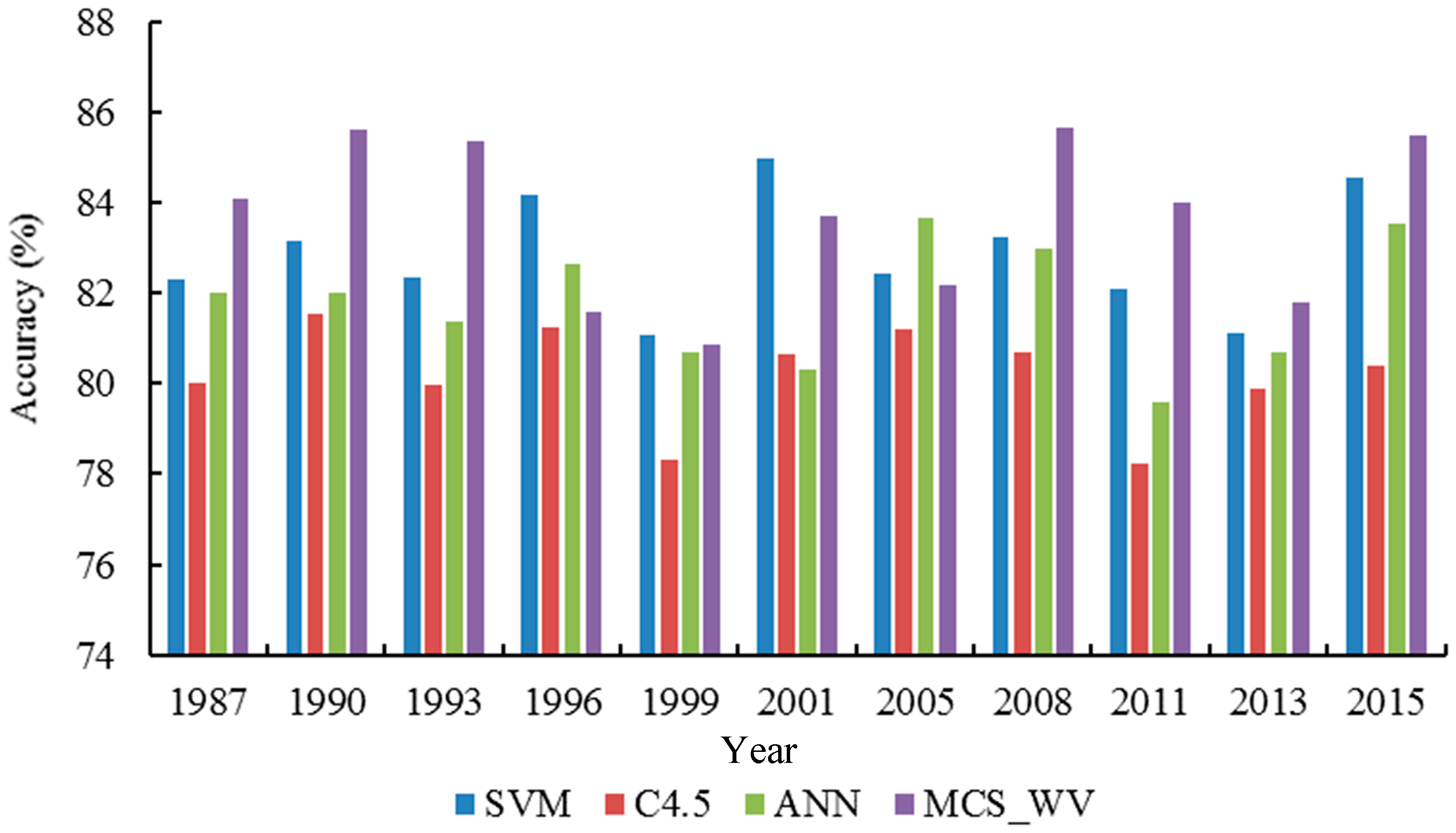
Although MCS_WV can obtain a higher classification accuracy over each base classifier, this boost may not applied to all cases, because the accuracies by MCS_WV for the 1996, 2001, 2005 and 2013 maps are lower than the highest accuracy by a base classifier (see Figure 7). This observation suggests that certain unstable factors may exist in the MCS_WV classification model. Presumably, the weight vector used in MCS_WV should be based on a large amount of a priori knowledge in calculating the recognition power for different base classifier. The higher representation of the training samples is, the better performance of MCS_WV could be. However, the objects on remote sensing images are so complexed that training samples may not represent the entire dataset well, which may lead the MCS_WV classifier to over fit. This further suggests that MCS_WV may lack robustness as its stability can be affected by less representative samples.
To analyze the classification performance of MCS_WV with two base classifiers, the average overall classification accuracies from three combinations are shown in Table 7. Based on Table 7, we can see that there is no significant improvement when MCS_WV was built upon the use of two base classifiers. This suggests that, if the number of base classifier is too small, the classification accuracy improvement by MCS_WV can be quite limited.
5.3. Performance of MCS_WV Improved by AdaBoost
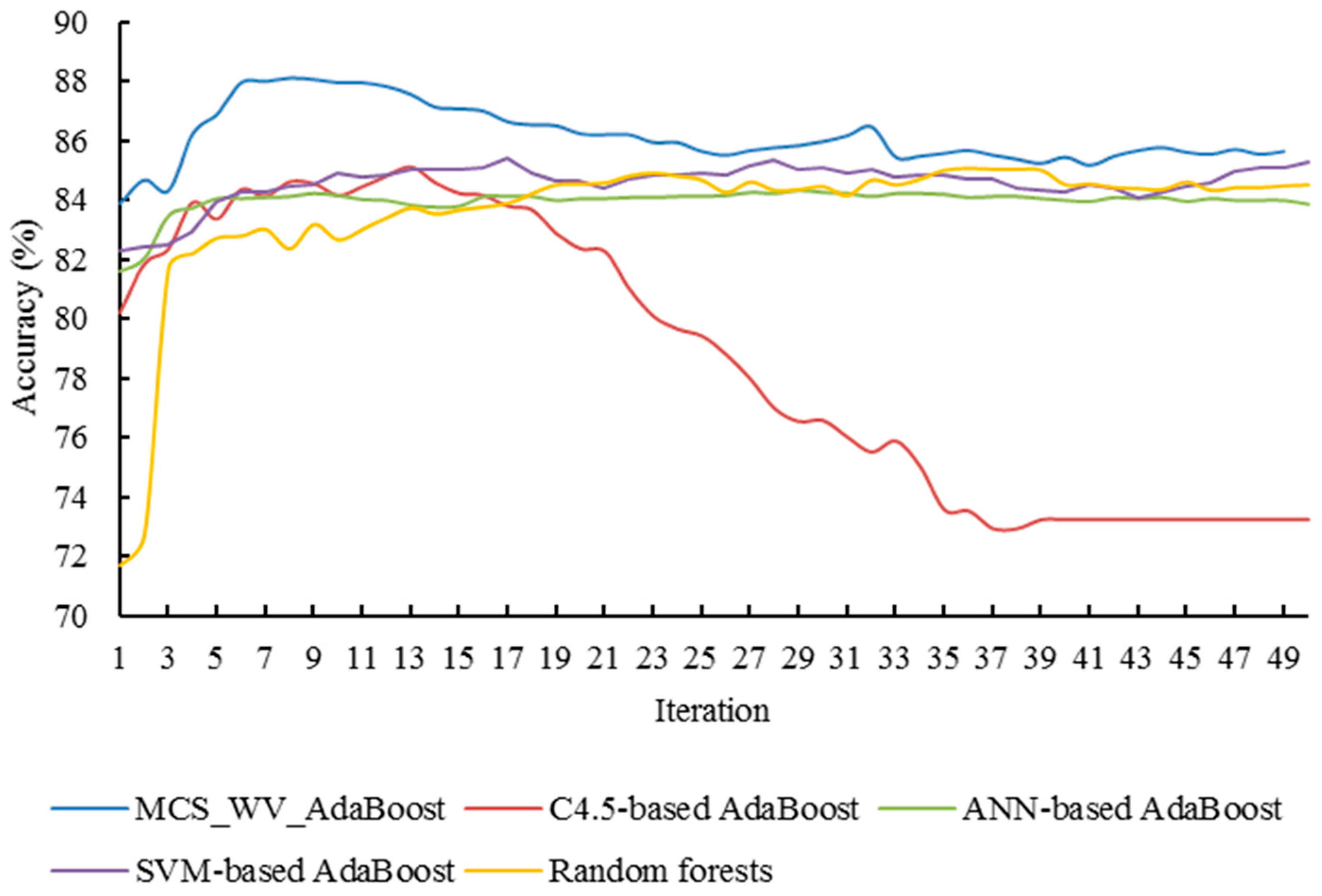
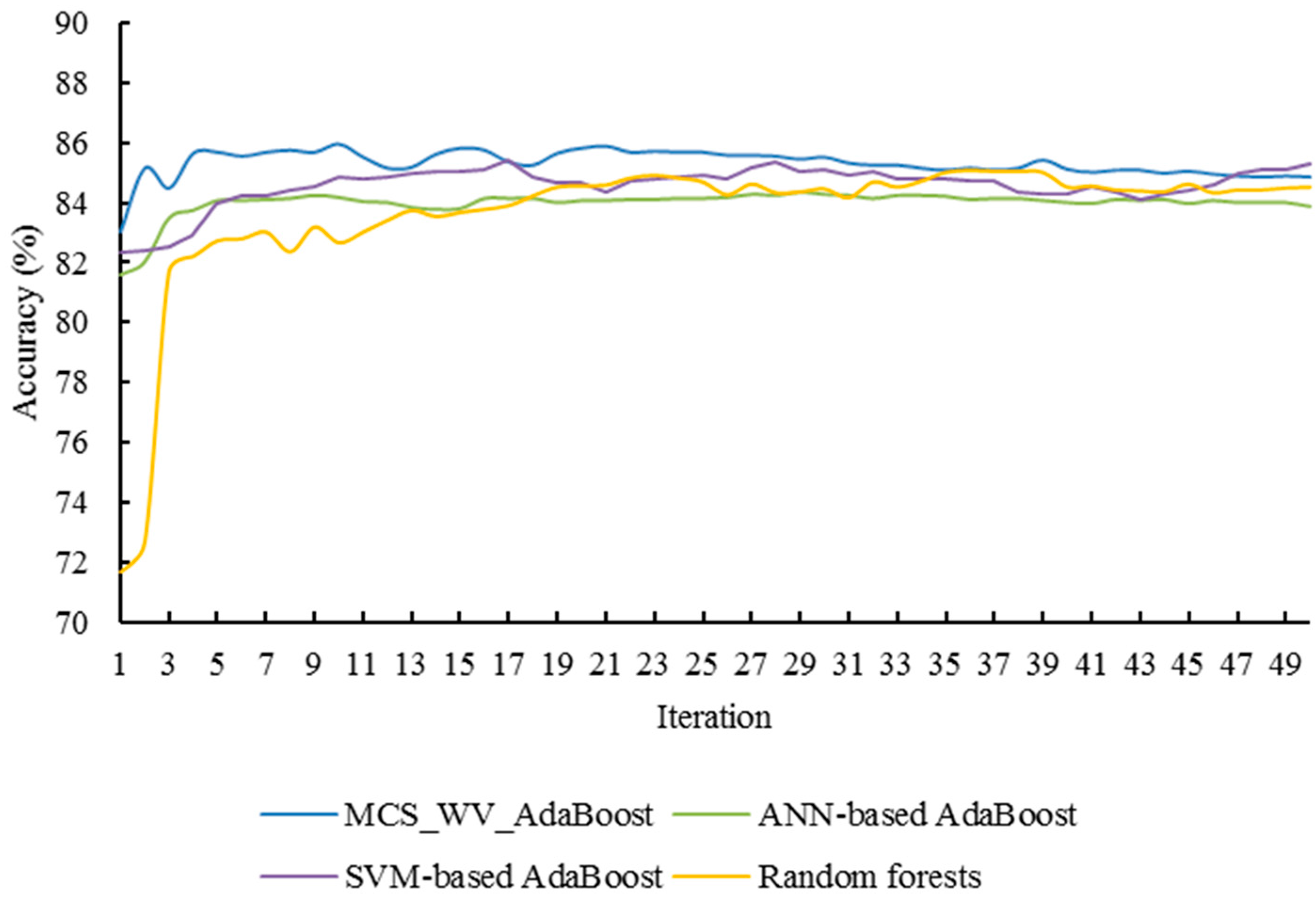
Setting the iterations of AdaBoost as 50, the relationship between the classification accuracy and the iteration number is illustrated in Figure 8, and the classification improvements of different AdaBoosts are also compared with the random forest (the maximum depth of each decision tree is 7, and the minimum simple count is 50; the total number of trees in a random forest is 50). Under eight iterations, MCS_WV_AdaBoost reached the highest classification accuracy (88.12%), which is 4.45% higher than single MCS_WV (83.67%). It is clear that MCS_WV performance boosting gradually increased as the iteration times increased, but the accuracy reached a ceiling point. When applying AdaBoost on C4.5, SVM or ANN, classification performance was also improved under several interactions. With C4.5-based AdaBoost, classification accuracy improved from 80.20 to 85% under 13 iterations. SVM-based AdaBoost increased classification accuracy from 82.85 to 85.41% with 17 iterations. Under 29 iterations, ANN-based AdaBoost improved classification accuracy from 81.77 to 84.34%. Clearly, MCS_WV_AdaBoost outperformed C4.5-, SVM-, and ANN-based AdaBoost, and needed fewer iterations to reach the highest classification accuracy.
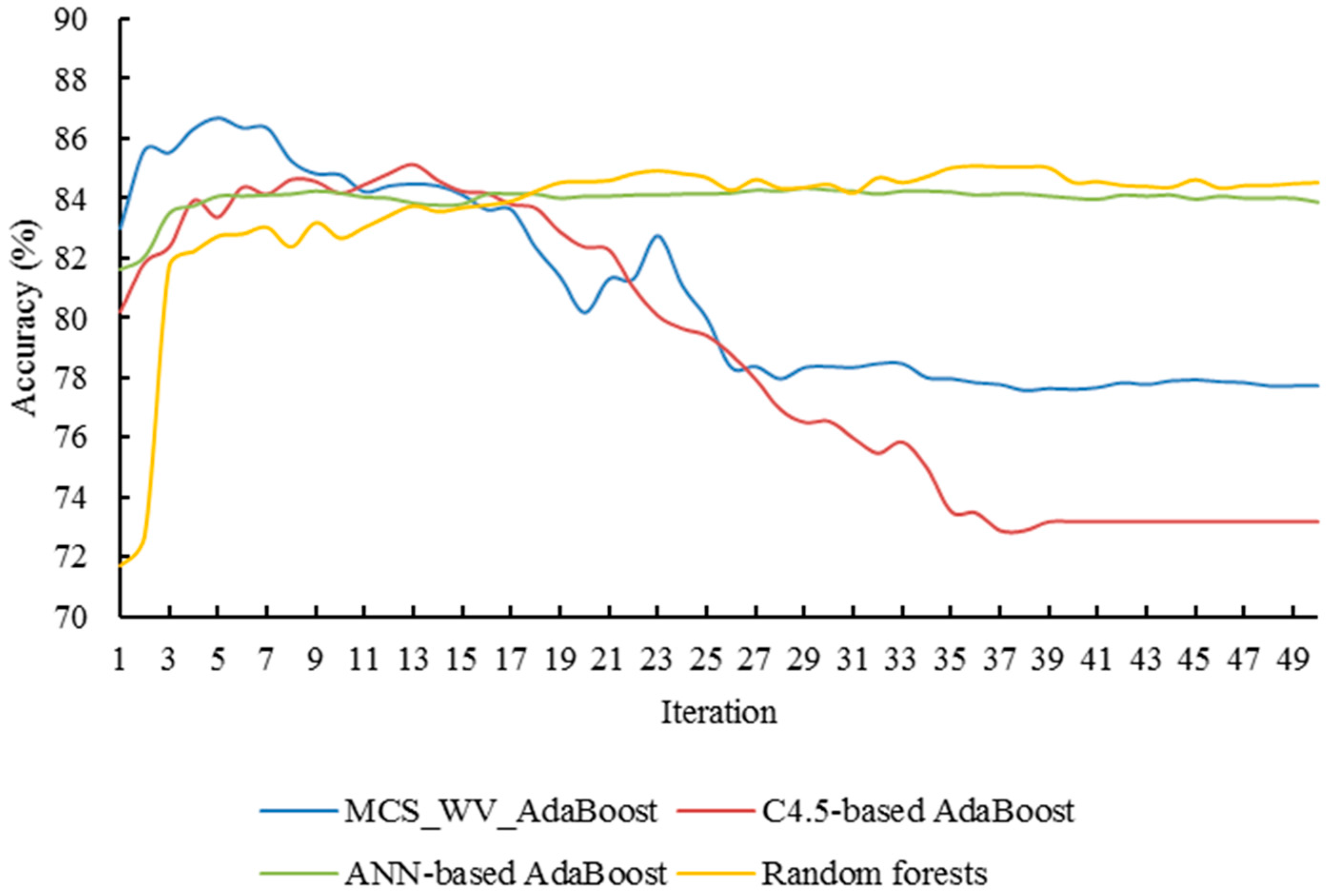
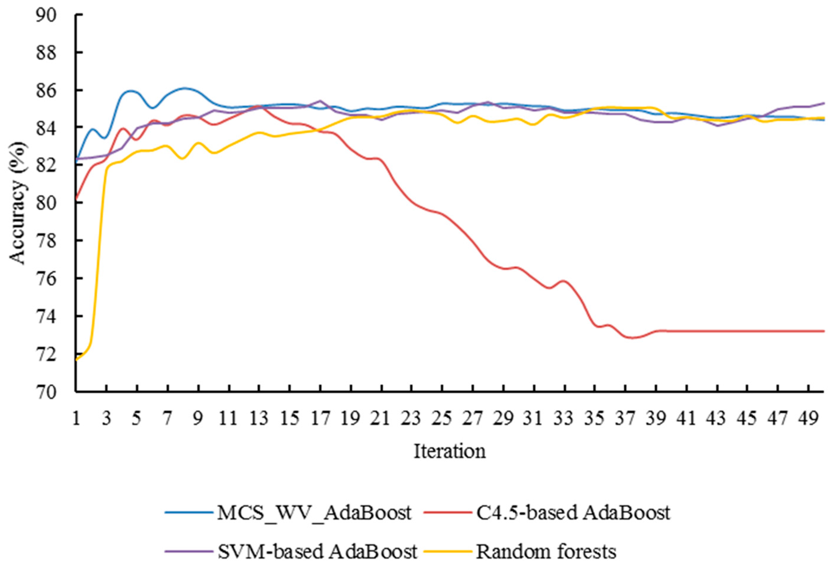
Figure 9, Figure 10 and Figure 11 show the performance of MCS_WV_AdaBoosts with two component classification algorithms. MCS_WV_AdaBoost with C4.5 and ANN improved the classification accuracy from 83.01 to 86.68% under eight iterations. MCS_WV_AdaBoost with C4.5 and SVM improved the classification accuracy from 82.98 to 86.08% under eight iterations. MCS_WV_AdaBoost with ANN and SVM boosted the classification accuracy from 82.11 to 85.97% under 10 iterations. While all these improvements are quite encouraging, MCS_WV_AdaBoost with C4.5, ANN, and SVM performed the best. It indicates that MCS_WV_AdaBoost can improve MCS_WV classification performance effectively and that the number of classifiers included in MCS_WV also affected the performance of MCS_WV_AdaBoost.
As shown in Figure 8, Figure 9, Figure 10 and Figure 11, MCS_WV_AdaBoost can reach its highest classification accuracy under few iterations. Random forest also achieves good classification performance. However, its highest accuracy, 85.0%, appears at the 39th iteration, which is lower than that of MCS_WV_AdaBoost. Compared with random forest, MCS_WV_AdaBoost cannot remain stable in its later iterations, because the overfitting nature of AdaBoost in later iterations has influenced classification accuracy improvement. This feature indicates that MCS_WV_AdaBoost is a classification algorithm which can work effectively in the early iterations.
Table 8 lists the computation time costs of different MCS_WV_AdaBoosts and the random forest. It indicates that MCS_WV_AdaBoosts cost more time for training than random forest within 50 iterations. When it comes to the highest classification accuracy, the number of iterations of MCS_WV_AdaBoost is smaller than that of random forests, but MCS_WV_AdaBoosts still show a feature of time-consuming. The time cost of MCS_WV_AdaBooost mainly depends on the learning algorithms of the base classifiers. As ANN and SVM require an excessive amount of time for training, MCS_WV_AdaBoosts that contain ANN and SVM are more time-consuming.
MCS_WV_AdaBoost perfectly inherited the benefits from MCS_WV and AdaBoost. First, with the weighted samples, MCS_WV in each subsequent iteration focused more on the samples being difficult to classify in the prior iteration. As a result, all MCS_WV classifiers are diverse in MCS_WV_AdaBoost. With weighted voting, the decisions of MCS_WV classifiers were combined and compared with any single MCS_WV classifier a more accurate result was generated. Second, under several iterations of MCS_WV_AdaBoost, overfitting of MCS_WV classifier that often caused by poor representation of training sample set was minimized. By combining a set of MCS_WV classifiers, MCS_WV_AdaBoost generated very strong performance. Because MCS_WV classifiers in MCS_WV_AdaBoost had a strong adaptive ability to the samples which are difficult to classify, they are focused on these specific samples rather than the whole sample set. In addition, due to MCS_WV, the advantages of SVM, C4.5 and ANN are complemented in MCS_WV_AdaBoost, which generated higher classification accuracy than any single classifiers. It can be explained that, for different classes, the sensitivity of different algorithms are different. With weight vectors, MCS_WV took the full use of the advantages from different classifiers, and these features were inherited by MCS_WV_AdaBoost successfully. In MCS_WV_AdaBoost, AdaBoost provided a classification accuracy boost mechanism for MCS_WV, and therefore, the advantages of MCS_WV were not affected but enhanced through combining various MCS_WVs decisions due to this mechanism. For example, built-up area (BA) and bare land (BL) were classified with lower accuracies by using SVM, C4.5 or ANN, but with MCS_WV_AdaBoost, the mapping accuracy of built-up area and bare land reached 92.99% and 88.11%, respectively, which are higher than those by any single classifiers (see Table 4). Accuracies of grassland (GR) and cultivated land (CL) were significantly improved. Comparing with the highest accuracy by single classifiers, using MCS_WV_AdaBoost classifier, the mapping accuracy of grassland (GR) and cultivated land (CL) was improved 6.1% and 5.9%, respectively. Obviously, MCS_WV_AdaBoost performed better for these classes with similar spectral characteristics. The improvement made for individual classes eventually helped improve the overall classification accuracy by MCS_WV_AdaBoost.
6. Conclusions
In this paper, a multiple classifiers system using SVM, C4.5 and ANN as base classifier and AdaBoost as the combination strategy, namely MCS_WV_AdaBoost, was proposed to derive land use/cover information from a time series of remote sensor images spanning a period from 1987 to 2015, with an average interval of three years. In total, 11 land use/cover maps were produced. The following conclusions have been made.
For the three base classifiers considered, SVM generated the highest average overall classification (82.85), followed by ANN (81.77%) and C4.5 decision tree (80.20%). These classifiers had their own advantages in mapping different LUC types. C4.5 outperformed the other two base classifiers in mapping built-up land. ANN generated the highest classification accuracy for grassland. SVM performed the best in classifying forest and cultivated land. All classifiers did well in mapping waters due to their unique spectral characteristics. Using C4.5 or ANN, built-up land and bare land can be clearly separated. These advantages by different classifiers for different classes were critical for MCS to generate improved classification accuracy.
The MCS_WV classifier was quite efficient in combining the results from different classifiers but its ensemble results can be affected by the representative of the training samples. If the representative is weak, the MCS_WV classifier could be overfitting. The AdaBoost algorithm can overcome this shortage by training more than one MCS_WV classifier. Compared with the individual MCS_WV classifier, MCS_WV_AdaBoost was more robust with higher classification accuracy.
With MCS_WV_AdaBoost, the classification accuracy was improved for each map, with the average overall accuracy higher than that from any base classifiers, which was due to the combined advantages from each base classifier. Based on the accuracy improvement of each class, the overall accuracy was improved by MCS_WV_AdaBoost. MCS_WV_AdaBoost generated higher classification accuracy, especially for those classes with similar spectral characteristics, such as built-up area and bare land, and cultivated land and grassland.
MCS_WV_AdaBoost inherited most benefits from MCS_WV and AdaBoost. However, it also suffers from some disadvantages. For example, it reduces but does not eliminate the overfitting inherited from AdaBoost; if noise exists in the samples, it has a tendency to overfit. In this paper, three classification algorithms were used to train base classifiers of MCS_WV, the performance of MCS_WV_AdaBoost worked on more classification algorithms still needs further study. In summary, with MCS_WV_AdaBoost, a reliable and accurate LUC data set of Guangzhou city was obtained, and could be used analyzing urban characteristics and urbanization effects upon the environment and ecosystem in the future studies.
Acknowledgments
This study is supported by the Natural Science Foundation of China (NSFC) (Funding No. 51379222), the National Science & Technology Pillar Program during the Twentieth Five-year Plan Period (Funding No. 2015BAK11B02) and the Science and Technology Program of Guangdong Province (Funding No. 2014A050503031).
Author Contributions
Yangbo Chen conceived this article; Peng Dou designed the methodologies, performed the algorithm programing, and analyzed the data and results; and Xiaojun Yang provided the necessary advice.
Conflicts of Interest
The authors declare no conflict of interest. The founding sponsors had no role in the design of the study; in the collection, analyses, or interpretation of data; in the writing of the manuscript, and in the decision to publish the results.
References
- Stow, D.A.; Chen, D.M. Sensitivity of multitemporal NOAA AVHRR data of an urbanizing region to land-use/land-cover changes and misregistration. Remote Sens. Environ. 2003, 80, 297–307. [Google Scholar] [CrossRef]
- Cofie, O. Dynamics of land-use and land-cover change in Freetown, Sierra Leone and its effects on urban and peri-urban agriculture—A remote sensing approach. Int. J. Remote Sens. 2011, 32, 1017–1037. [Google Scholar]
- Kaźmierczak, A.; Cavan, G. Surface water flooding risk to urban communities: Analysis of vulnerability, hazard and exposure. Landsc. Urban Plan. 2001, 11, 185–197. [Google Scholar] [CrossRef]
- Huang, J.L.; Klemas, V. Using remote sensing of land cover change in coastal watersheds to predict downstream water quality. J. Coast. Res. 2012, 28, 930–944. [Google Scholar] [CrossRef]
- Bateni, F.; Fakheran, S.; Soffianian, A. Assessment of land cover changes & water quality changes in the Zayandehroud River Basin between 1997–2008. Environ. Monit. Assess. 2013, 185, 105–119. [Google Scholar]
- Treitz, P.M.; Howard, P.J.; Gong, P. Application of satellite and GIS technologies for land-cover and land use mapping at the rural-urban fringe: A case study. Photogramm. Eng. Remote Sens. 1992, 58, 439–448. [Google Scholar]
- Mohan, M.; Kikegawa, Y.; Gurjar, B.R.; Bhati, S.; Kolli, N.R. Assessment of urban heat island effect for different land use–land cover from micrometeorological measurements and remote sensing data for megacity Delhi. Theor. Appl. Climatol. 2013, 112, 647–658. [Google Scholar] [CrossRef]
- Usman, M.; Liedel, R.; Shahid, M.A.; Abbas, A. Land use/land cover classification and its change detection using multi-temporal MODIS NDVI data. J. Geogr. Sci. 2015, 25, 1479–1506. [Google Scholar] [CrossRef]
- Boori, M.S.; Voženílek, V.; Choudhary, K. Land use/cover disturbance due to tourism in Jeseníky Mountain, Czech Republic: A remote sensing and GIS based approach. Egypt. J. Remote Sens. 2014, 23, 17–26. [Google Scholar] [CrossRef]
- Chander, G.; Markham, B.L.; Helder, D.L. Summary of current radiometric calibration coefficients for Landsat MSS, TM, ETM+, and EO-1 ALI sensors. Remote Sens. Environ. 2009, 113, 893–903. [Google Scholar] [CrossRef]
- Badreldin, N.; Goossens, R. Monitoring land use/land cover change using multi-temporal Landsat satellite images in an arid environment: A case study of El-Arish, Egypt. Arab. J. Geosci. 2014, 7, 1671–1681. [Google Scholar] [CrossRef]
- Nutini, F.; Boschetti, M.; Brivio, P.A.; Bocchi, S.; Antoninetti, M. Land-use and land-cover change detection in a semi-arid area of Niger using multi-temporal analysis of Landsat images. Int. J. Remote Sens. 2013, 34, 4769–4790. [Google Scholar] [CrossRef]
- Xia, J.S.; Mura, M.D.; Chanussot, J.; Du, P.; He, X. Random subspace ensembles for hyperspectral image classification with extended morphological attribute profiles. IEEE Trans. Geosci. Remote Sens. 2015, 53, 4768–4786. [Google Scholar] [CrossRef]
- Duro, D.C.; Franklin, S.E.; Dubé, M.G. A comparison of pixel-based and object-based image analysis with selected machine learning algorithms for the classification of agricultural landscapes using SPOT-5 HRG imagery. Remote Sens. Environ. 2012, 118, 259–272. [Google Scholar] [CrossRef]
- Ghosh, A.A.; Ghosh, S. Supervised and unsupervised land-use map generation from remotely sensed images using ant based systems. Appl. Soft Comput. 2011, 11, 5770–5781. [Google Scholar]
- Waske, B.; Linden, S.V.D.; Benediktsson, J.A.; Rabe, A.; Hostert, P. Sensitivity of support vector machines to random feature selection in classification of hyperspectral data. IEEE Trans. Geosci. Remote Sens. 2010, 7, 2880–2889. [Google Scholar] [CrossRef]
- Mazzoni, D.; Garay, M.J.; Davies, R.; Nelson, D. An operational MISR pixel classifier using support vector machines. Remote Sens. Environ. 2007, 107, 149–158. [Google Scholar] [CrossRef]
- Gomez-Chova, L.; Camps-Valls, G. Semi supervised image classification with Laplacian support vector machines. IEEE Geosci. Remote Sens. 2008, 5, 336–340. [Google Scholar] [CrossRef]
- Ding, Z.J.; Yu, J.; Zhang, Y. A new improved k-means algorithm with penalized term. In Proceedings of the IEEE International Conference on Granular Computing, Fremont, CA, USA, 2–4 November 2007; pp. 313–317. [Google Scholar]
- Thitimajshima, P. A new modified fuzzy c-means algorithm for multispectral satellite images segmentation. In Proceedings of the IEEE 2000 International Geoscience and Remote Sensing Symposium, Honolulu, HI, USA, 24–28 July 2000; pp. 1684–1686. [Google Scholar]
- Yang, C.; Bruzzone, L.; Sun, F.Y.; Liang, Y. A fuzzy-statistics-based affinity propagation technique for clustering in multispectral images. IEEE Trans. Geosci. Remote Sens. 2010, 48, 2647–2659. [Google Scholar] [CrossRef]
- Shahshahani, B.; Landgrebe, D. The effect of unlabeled sample in reducing the small sample size problem and mitigating the Hughes phenomenon. IEEE Trans. Geosci. Remote Sens. 1994, 32, 1087–1095. [Google Scholar] [CrossRef]
- Pal, M.; Mather, P.M. Support vector machines for classification in remote sensing. Int. J. Remote Sens. 2005, 26, 1007–1011. [Google Scholar] [CrossRef]
- Tong, X.; Zhang, X.; Liu, M. Detection of urban sprawl using a genetic algorithm-evolved artificial neural network classification in remote sensing: A case study in Jiading and Putuo districts of Shanghai, China. Int. J. Remote Sens. 2010, 31, 1485–1504. [Google Scholar] [CrossRef]
- Giacinto, G.; Roli, F.; Vernazza, G. Comparison and combination of statistical and neural network algorithms for remote-sensing image classification. In Neurocomputation in Remote Sensing Data Analysis; Springer: Berlin/Heidelberg, Germany, 1997; pp. 117–124. [Google Scholar]
- Du, P.; Xia, J.S.; Zhang, W.; Tan, K.; Liu, Y. Multiple classifier system for remote sensing image classification: An review. Sensors 2012, 26, 4764–4792. [Google Scholar] [CrossRef] [PubMed]
- Biggio, B.; Fumera, G.; Roli, F. Multiple classifier systems for robust classifier design in adversarial environments. Int. J. Mach. Learn. Cybern. 2010, 1, 27–41. [Google Scholar] [CrossRef]
- Xiao, H.; Zhang, X. Comparison studies on classification for remote sensing image based on data mining method. WSEAS Trans. Comput. 2008, 7, 552–558. [Google Scholar]
- Debeir, O.; Latinne, P.; Steen, I.V.D. Remote sensing classification of spectral, spatial and contextual data using multiple classifier systems. In Proceedings of the 8th ECS and Image Analysis, Bordeaux, France, 4–7 September 2001; pp. 584–589. [Google Scholar]
- Nie, W.; Yuan, Y.; Kepner, W.G.; Nash, M.; Jackson, M.; Torkildson, C. Assessing impacts of landuse and landcover changes on hydrology for the Upper San Pedro Watershed. J. Hydrol. 2011, 407, 105–114. [Google Scholar]
- Windeatt, T. Diversity measures for multiple classifier system analysis and design. Inf. Fusion 2005, 6, 21–36. [Google Scholar] [CrossRef]
- Tan, K.; Jin, X.; Plaza, A.; Wang, X.; Xiao, L. Automatic change detection in high-resolution remote sensing images by using a multiple classifier system and spectral–spatial Features. IEEE J. Sel. Top. Appl. Earth Obs. Remote Sens. 2016, 9, 3439–3451. [Google Scholar] [CrossRef]
- Du, P.; Samat, A.; Waske, B.; Liu, S.; Li, Z. Random Forest and Rotation Forest for fully polarized SAR image classification using polarimetric and spatial features. ISPRS J. Photogramm. Remote Sens. 2015, 105, 38–53. [Google Scholar] [CrossRef]
- Foody, G.M.; Boyd, D.S.; Sanchez-Hernandez, C. Mapping a specific class with an ensemble of classifiers. Int. J. Remote Sens. 2007, 28, 1733–1746. [Google Scholar] [CrossRef]
- Maulik, U.; Chakraborty, D. A robust multiple classifier system for pixel classification of remote sensing images. Fund. Inform. 2010, 101, 286–304. [Google Scholar]
- Li, F.; Xu, L.; Siva, P.; Wong, A.; Clausi, D.A. Hyperspectral image classification with limited labeled training samples using enhanced ensemble learning and conditional random fields. IEEE J. Sel. Top. Appl. Earth Obs. Remote Sens. 2015, 8, 2427–2438. [Google Scholar] [CrossRef]
- Fersini, E.; Messina, E.; Pozzi, F.A. Sentiment analysis: Bayesian ensemble learning. Decis. Support Syst. 2014, 68, 26–38. [Google Scholar] [CrossRef]
- Naeini, M.P.; Moshiri, B.; Araabi, B.N.; Sadeghi, M. Learning by abstraction: Hierarchical classification model using evidential theoretic approach and Bayesian ensemble model. Neurocomputing 2014, 130, 73–82. [Google Scholar] [CrossRef]
- Papageorgiou, E.I.; Kannappan, A. Fuzzy cognitive map ensemble learning paradigm to solve classification problems: Application to autism identification. Appl. Soft Comput. 2013, 12, 3798–3809. [Google Scholar] [CrossRef]
- Li, M.; Zhou, Z.H. Improve computer-aided diagnosis with machine learning techniques using undiagnosed samples. IEEE Trans. Syst. Man Cybern. Part A Syst. Hum. 2007, 37, 1088–1098. [Google Scholar] [CrossRef]
- Dai, L.; Liu, C. Multiple classifier combination for land cover classification of remote sensing image. In Proceedings of the 2010 2nd International Conference on Information Science and Engineering (ICISE), Hangzhou, China, 4–6 December 2010; pp. 3835–3839. [Google Scholar]
- Zhao, Q.; Song, W. Remote sensing image classification based on multiple classifiers fusion. In Proceedings of the 2010 3rd International Congress on Image and Signal Processing (CISP), Yantai, China, 16–18 October 2010; pp. 1927–1931. [Google Scholar]
- Kumar, D.A.; Meher, S.K. Multiple classifiers systems with granular neural networks. In Proceedings of the 2013 IEEE International Conference on Signal Processing, Computing and Control (ISPCC), Solan, India, 26–28 September 2013; pp. 1–5. [Google Scholar]
- Ceamanos, X.; Waske, B.; Benediktsson, J.A.; Chanussot, J.; Fauvel, M.; Sveinsson, J.R. A classifier ensemble based on fusion of support vector machines for classifying hyperspectral data. Int. J. Image Data Fusion 2010, 1, 293–307. [Google Scholar] [CrossRef] [Green Version]
- Kuncheva, L.I. Diversity in multiple classifier systems. Inf. Fusion 2005, 6, 3–4. [Google Scholar] [CrossRef]
- Chan, C.W.; Paelinckx, D. Evaluation of random forest and Adaboost tree-based ensemble classification and spectral band selection for ecotope mapping using airborne hyperspectral imagery. Remote Sens. Environ. 2008, 112, 2999–3011. [Google Scholar] [CrossRef]
- Huang, J.; Wang, M.; Gu, B.; Chen, Z.; Huang, J. Multiple classifiers combination based on interval-valued fuzzy permutation. J. Comput. Inf. Syst. 2010, 6, 1759–1768. [Google Scholar]
- Tai, F.; Pan, W. Incorporating prior knowledge of predictors into penalized classifiers with multiple penalty terms. Bioinformatics 2007, 23, 1775–1782. [Google Scholar] [CrossRef] [PubMed]
- Vuolo, F.; Atzberger, C. Exploiting the classification performance of support vector machines with multi-temporal Moderate-Resolution Imaging Spectroradiometer (MODIS) Data in areas of agreement and disagreement of existing land cover products. Remote Sens. 2012, 4, 3143–3167. [Google Scholar] [CrossRef]
- Kavzoglu, T.; Colkesen, I.; Yomralioglu, T. Object-based classification with rotation forest ensemble learning algorithm using very-high-resolution WorldView-2 image. Remote Sens. Lett. 2015, 6, 838–843. [Google Scholar] [CrossRef]
- Nowakowski, A. Remote sensing data binary classification using Boosting with simple classifiers. Acta Geophys. 2015, 63, 1447–1462. [Google Scholar] [CrossRef]
- Kawaguchi, S.; Nishii, R. Hyperspectral image classification by bootstrap AdaBoost with random decision stumps. IEEE Trans. Geosci. Remote Sens. 2007, 45, 3845–3851. [Google Scholar] [CrossRef]
- Tzeng, Y.C.; Chiu, S.H.; Chen, K.S. Improvement of remote sensing image classification accuracy by using a multiple classifiers system with modified Bagging and Boosting algorithms. In Proceedings of the IEEE International Conference on Geoscience and Remote Sensing Symposium(IGARSS), Denver, CO, USA, 31 July–4 August 2006; pp. 2769–2772. [Google Scholar]
- Ghimire, B.; Rogan, J.; Rodriguez-Galiano, V.F.R.; Panday, P.; Neeti, N. An evaluation of bagging, boosting, and random forests for land-cover classification in cape cod, Massachusetts, USA. Gisci. Remote Sens. 2012, 49, 623–643. [Google Scholar] [CrossRef]
- Khosravi, I.; Mohammad-Beigi, M. Multiple classifier systems for hyperspectral remote sensing data classification. J. Indian Soc. Remote Sens. 2014, 42, 423–428. [Google Scholar] [CrossRef]
- Xia, J.S.; Du, P.; He, X.; Chanussot, J. Hyperspectral remote sensing image classification based on rotation forest. IEEE Geosci. Remote Sens. 2014, 11, 239–243. [Google Scholar] [CrossRef]
- Briem, G.; Benediktsson, J.; Sveinsson, J. Multiple classifiers applied to multisource remote sensing data. IEEE Trans. Geosci. Remote Sens. 2002, 40, 2291–2299. [Google Scholar] [CrossRef]
- Benediktsson, J.A.; Chanussot, J.; Fauvel, M. Multiple classifier systems in remote sensing: From basics to recent developments. In Proceedings of the 7th International Workshop on Multiple Classifier Systems, Prague, Czech Republic, 23–25 May 2007; pp. 501–502. [Google Scholar]
- Sankhua, R.N.; Sharma, N.; Garg, P.K.; Pandey, A.D. Use of remote sensing and ANN in assessment of erosion activities in Majuli, the world’s largest river island. Int. J. Remote Sens. 2010, 26, 4445–4454. [Google Scholar] [CrossRef]
- Moustakidis, S.; Mallinis, G.; Koutsias, N.; Theocharis, J.B. SVM-based fuzzy decision trees for classification of high spatial resolution remote sensing images. IEEE Trans. Geosci. Remote Sens. 2012, 50, 149–169. [Google Scholar] [CrossRef]
- Jiang, L.; Wang, W.; Yang, X.; Xie, N.; Cheng, Y. Classification Methods of Remote Sensing Image Based on Decision Tree Technologies. Agric. Netw. Inf. 2009, 22, 4058–4061. [Google Scholar]
- Vapnik, V.N. Statistical learning theory. Encycl. Sci. Learn. 1999, 41, 3185. [Google Scholar]
- Buddhiraju, K.M.; Rizvi, I.A. Comparison of CBF, ANN and SVM classifiers for object based classification of high resolution satellite images. In Proceedings of the IEEE International Geoscience and Remote Sensing Symposium, Honolulu, HI, USA, 25–30 July 2010; pp. 40–43. [Google Scholar]
- Dou, P.; Zhai, L.; Sang, H.; Xie, W. Research and application of Object-oriented remote sensing image classification based on decision tree. In Proceedings of the 2013 International Conference on Remote Sensing, Environment and Transportation Engineering, Nanjing, China, 26–28 July 2013; pp. 272–275. [Google Scholar]
- Şahin, M. Modelling of air temperature using remote sensing and artificial neural network in Turkey. Adv. Space Res. 2012, 50, 973–985. [Google Scholar] [CrossRef]
- Palani, S.; Tkalich, P.; Balasubramanian, R.; Palanichamy, J. ANN application for prediction of atmospheric nitrogen deposition to aquatic ecosystems. Mar. Pollut. Bull. 2011, 62, 1198–1206. [Google Scholar] [CrossRef] [PubMed]
- Coppin, P.; Jonckheere, I.; Nackaerts, K.; Muys, B.; Lambin, E. Digital change detection methods in ecosystem monitoring: A review. Int. J. Remote Sens. 2010, 25, 1565–1596. [Google Scholar] [CrossRef]
- Fan, T.G.; Zhu, Y.; Chen, J.M. A new measure of classifier diversity in multiple classifier system. In Proceedings of the 2008 International Conference on Machine Learning and Cybernetics, Kunming, China, 12–15 July 2008; pp. 18–21. [Google Scholar]
- Freund, Y. Boosting a weak learning algorithm by majority. Inf. Comput. 1997, 21, 256–285. [Google Scholar]
- Isaac, E.; Easwarakumar, K.S.; Isaac, J. Urban landcover classification from multispectral image data using optimized AdaBoosted random forests. Remote Sens. Lett. 2017, 8, 350–359. [Google Scholar] [CrossRef]
- Owusu, E.; Zhan, Y.; Mao, Q.R. A neural-AdaBoost based facial expression recognition system. Expert Syst. Appl. 2014, 41, 3383–3390. [Google Scholar] [CrossRef]
- Ramzi, P.; Samadzadegan, F.; Reinartz, P. Classification of hyperspectral data using an AdaBoost SVM technique applied on band closers. IEEE J. Sel. Top. Appl. 2014, 7, 2066–2079. [Google Scholar]
- Damodaran, B.B.; Nidamanuri, R.R. Dynamic Linear Classifier System for Hyperspectral Image Classification for Land Cover Mapping. IEEE J. Sel. Top. Appl. Earth Obs. Remote Sens. 2014, 7, 2080–2093. [Google Scholar] [CrossRef]
- Szuster, B.; Chen, W.Q.; Borger, M. A comparison of classification techniques to support land cover and land use analysis in tropical coastal zones. Appl. Geogr. 2011, 31, 525–532. [Google Scholar] [CrossRef]
Figure 1.
Location of the study area (the geographic extent is 113°8′43″E to 113°30′39″E and 23°2′30″N to 23°25′40″N).
Figure 1.
Location of the study area (the geographic extent is 113°8′43″E to 113°30′39″E and 23°2′30″N to 23°25′40″N).

Figure 2.
Flow chart of the research procedural route.

Figure 3.
Diagram of MCS_WV (multiple classifiers system based on weight vector) classification.

Figure 4.
Diagram of MCS_WV_AdaBoost (MCS_WV improved by AdaBoost) training.

Figure 5.
Land use/cover maps for the Guangzhou metropolitan area in 2001 produced using different classifiers: (a) SVM; (b) C4.5; (c) ANN; and (d) MCS_WV AdaBoost (MCS_WV improved by AdaBoost).
Figure 5.
Land use/cover maps for the Guangzhou metropolitan area in 2001 produced using different classifiers: (a) SVM; (b) C4.5; (c) ANN; and (d) MCS_WV AdaBoost (MCS_WV improved by AdaBoost).

Figure 6.
Land use/cover maps for the Guangzhou metropolitan area from 1987 to 2015.

Figure 7.
Overall classification accuracies by SVM, C4.5, ANN and MCS_WV for different years.

Figure 8.
Classification accuracy improvements of MCS_WV_AdaBoost using three base classifier training algorithms: C4.5, ANN and SVM.
Figure 8.
Classification accuracy improvements of MCS_WV_AdaBoost using three base classifier training algorithms: C4.5, ANN and SVM.

Figure 9.
Classification accuracy improvements of MCS_WV_AdaBoost using two base classifier training algorithms: C4.5 and ANN.
Figure 9.
Classification accuracy improvements of MCS_WV_AdaBoost using two base classifier training algorithms: C4.5 and ANN.

Figure 10.
Classification accuracy improvements of MCS_WV_AdaBoost using two base classifier training algorithms: C4.5 and SVM.
Figure 10.
Classification accuracy improvements of MCS_WV_AdaBoost using two base classifier training algorithms: C4.5 and SVM.

Figure 11.
Classification accuracy improvements of MCS_WV_AdaBoost using two base classifier training algorithms: ANN and SVM.
Figure 11.
Classification accuracy improvements of MCS_WV_AdaBoost using two base classifier training algorithms: ANN and SVM.


Table 1.
Landsat images acquired.
| Platform | Sensor | Bands | Spatial Resolution (m) | Acquisition Year |
|---|---|---|---|---|
| Landsat 5 | TM | 1–5, 7 | 30 | 1987, 1990, 1993, 1996, 1999, 2005, 2008, 2011 |
| Landsat 7 | ETM+ | 1–5, 7 | 30 | 2001 |
| Landsat 8 | OLI | 2–6, 7 | 30 | 2013, 2015 |
Table 2.
Number of samples in training sets.
| Year | BA | WA | GR | FO | BL | CL | Total |
|---|---|---|---|---|---|---|---|
| 1988 | 189 | 201 | 211 | 198 | 202 | 210 | 1211 |
| 1990 | 200 | 208 | 195 | 215 | 218 | 189 | 1225 |
| 1993 | 213 | 216 | 208 | 201 | 220 | 190 | 1248 |
| 1996 | 199 | 206 | 216 | 213 | 180 | 209 | 1223 |
| 1999 | 205 | 210 | 228 | 205 | 202 | 200 | 1250 |
| 2001 | 218 | 211 | 207 | 203 | 215 | 203 | 1257 |
| 2005 | 220 | 202 | 211 | 211 | 193 | 211 | 1248 |
| 2008 | 216 | 185 | 220 | 193 | 216 | 209 | 1239 |
| 2011 | 199 | 203 | 216 | 211 | 207 | 205 | 1241 |
| 2013 | 205 | 225 | 222 | 203 | 199 | 203 | 1257 |
| 2015 | 213 | 203 | 202 | 206 | 200 | 206 | 1230 |
Table 3.
Thematic mapping accuracies by different classifiers.
| Classifiers | ||||||||
|---|---|---|---|---|---|---|---|---|
| SVM | C4.5 | ANN | MCS_WV_AdaBoost | |||||
| Year | OA (%) | Kappa | OA (%) | Kappa | OA (%) | Kappa | OA (%) | Kappa |
| 1987 | 82.32 | 0.809 | 80.03 | 0.796 | 82.01 | 0.821 | 87.33 | 0.861 |
| 1990 | 83.15 | 0.823 | 81.55 | 0.812 | 81.99 | 0.803 | 90.64 | 0.889 |
| 1993 | 82.33 | 0.812 | 79.98 | 0.791 | 81.35 | 0.801 | 87.22 | 0.869 |
| 1996 | 84.15 | 0.839 | 81.23 | 0.813 | 82.65 | 0.821 | 90.12 | 0.883 |
| 1999 | 81.07 | 0.801 | 78.33 | 0.774 | 80.69 | 0.785 | 86.55 | 0.859 |
| 2001 | 84.98 | 0.829 | 80.63 | 0.792 | 80.33 | 0.799 | 90.01 | 0.893 |
| 2005 | 82.42 | 0.802 | 81.22 | 0.805 | 83.66 | 0.830 | 86.33 | 0.852 |
| 2008 | 83.22 | 0.819 | 80.69 | 0.801 | 82.96 | 0.812 | 86.59 | 0.851 |
| 2011 | 82.09 | 0.813 | 78.23 | 0.776 | 79.58 | 0.788 | 88.01 | 0.859 |
| 2013 | 81.11 | 0.808 | 79.88 | 0.765 | 80.67 | 0.791 | 86.34 | 0.849 |
| 2015 | 84.56 | 0.832 | 80.38 | 0.788 | 83.55 | 0.829 | 90.23 | 0.888 |
| Average | 82.85 | 0.817 | 80.20 | 0.792 | 81.77 | 0.807 | 88.12 | 0.868 |
Note: OA is abbreviation of “overall accuracy”.
Table 4.
Classification average producer’s accuracy with different classification algorithms.
| Classifiers | Average Producer’s Accuracy (%) | OA (%) | |||||
|---|---|---|---|---|---|---|---|
| BA | WA | GR | FO | BL | CL | ||
| C4.5 | 88.99 | 91.89 | 77.31 | 74.51 | 83.58 | 70.32 | 80.20 |
| SVM | 78.81 | 91.40 | 80.22 | 88.24 | 79.95 | 85.17 | 82.85 |
| ANN | 80.17 | 90.20 | 85.18 | 81.38 | 84.37 | 80.57 | 81.77 |
| MCS_WV | 87.33 | 94.50 | 87.22 | 88.38 | 85.07 | 86.11 | 83.67 |
| MCS_WV_AdaBoost | 92.99 | 98.20 | 91.18 | 89.13 | 88.11 | 86.24 | 88.12 |
Note: OA is abbreviation of “overall accuracy”; BA, WA, GR, FO, BL, and CL mean built-up area, water, grassland, forest, bare land and cultivated land, respectively.
Table 5.
Classification average user’s accuracy with different classification algorithms.
| Classifiers | Average User’s Accuracy (%) | OA (%) | |||||
|---|---|---|---|---|---|---|---|
| BA | WA | GR | FO | BL | CL | ||
| C4.5 | 89.12 | 90.44 | 73.28 | 80.01 | 82.01 | 75.34 | 80.20 |
| SVM | 77.33 | 92.01 | 83.37 | 87.29 | 73.55 | 84.02 | 82.85 |
| ANN | 79.26 | 90.59 | 86.09 | 80.03 | 80.23 | 81.25 | 81.77 |
| MCS_WV | 84.17 | 93.98 | 88.33 | 86.63 | 83.59 | 86.66 | 83.67 |
| MCS_WV_AdaBoost | 93.23 | 98.76 | 90.72 | 87.84 | 89.75 | 87.89 | 88.12 |
Note: BA, WA, GR, FO, BL, and CL mean built-up area, water, grassland, forest, bare land and cultivated land respectively.
Table 6.
The average contribution by each base classifier in MCS_WV for each land use/cover class.
| Classifiers | Land Use/Cover Class | |||||
|---|---|---|---|---|---|---|
| BA | WA | GR | FO | BL | CL | |
| C4.5 | 0.421 | 0.329 | 0.255 | 0.202 | 0.358 | 0.271 |
| SVM | 0.267 | 0.330 | 0.434 | 0.263 | 0.254 | 0.428 |
| ANN | 0.312 | 0.341 | 0.311 | 0.535 | 0.388 | 0.301 |
Note: BA, WA, GR, FO, BL and CL mean built-up area, water, grassland, forest, bare land and cultivated land, respectively.
Table 7.
MCS_WV classification accuracy with two base classifiers.
| Accuracy | Base Classifiers | ||
|---|---|---|---|
| ANN, SVM | C4.5, SVM | C4.5, ANN | |
| OA (%) | 82.11 | 82.98 | 83.01 |
| Kappa | 80.88 | 0.801 | 0.815 |
Table 8.
Computation time costs of different MCS_WV_AdaBoosts and the random forest.
| Learning Algorithm | Boosting Method | NIHCA | TC_NIHCA (ms) | TC_50 (ms) |
|---|---|---|---|---|
| C4.5 | AdaBoost | 13 | 305 | 1425 |
| SVM | AdaBoost | 28 | 2878 | 5350 |
| ANN | AdaBoost | 30 | 4201 | 12,214 |
| C4.5, ANN, and SVM | MCS_WV_AdaBoost | 8 | 3525 | 18,025 |
| C4.5 and ANN | MCS_WV_AdaBoost | 5 | 1476 | 13,762 |
| C4.5 and SVM | MCS_WV_AdaBoost | 8 | 1288 | 8703 |
| ANN and SVM | MCS_WV_AdaBoost | 10 | 3016 | 14,289 |
| Radom forest | None | 36 | 1523 | 3024 |
Note: NIHCA means the number of iterations to achieve highest classification accuracy and TC_NIHCA means the corresponding time cost; TC_50 means the time cost under 50 interactions.
© 2017 by the authors. Licensee MDPI, Basel, Switzerland. This article is an open access article distributed under the terms and conditions of the Creative Commons Attribution (CC BY) license (http://creativecommons.org/licenses/by/4.0/).
Share and Cite
MDPI and ACS Style
Chen, Y.; Dou, P.; Yang, X. Improving Land Use/Cover Classification with a Multiple Classifier System Using AdaBoost Integration Technique. Remote Sens. 2017, 9, 1055. https://0-doi-org.brum.beds.ac.uk/10.3390/rs9101055
AMA Style
Chen Y, Dou P, Yang X. Improving Land Use/Cover Classification with a Multiple Classifier System Using AdaBoost Integration Technique. Remote Sensing. 2017; 9(10):1055. https://0-doi-org.brum.beds.ac.uk/10.3390/rs9101055
Chicago/Turabian StyleChen, Yangbo, Peng Dou, and Xiaojun Yang. 2017. "Improving Land Use/Cover Classification with a Multiple Classifier System Using AdaBoost Integration Technique" Remote Sensing 9, no. 10: 1055. https://0-doi-org.brum.beds.ac.uk/10.3390/rs9101055
Note that from the first issue of 2016, this journal uses article numbers instead of page numbers. See further details here.