
Hydrological Modelling using Satellite-Based Crop Coefficients: A Comparison of Methods at the Basin Scale


 ,
,
Abstract
:
1. Introduction
2. Methods
2.1. Study Area
2.2. Hydrological Model and Input Data
2.3. Crop Coefficient Parameterization Methods
2.4. Reference Model Calibration and Validation
- -
- NSE: Nash-Sutcliffe efficiency (>0.50).
- -
- PBIAS: the percent bias (<25% or >−25%),
- -
- RSR: ratio of the root mean square error to the standard deviation of measured data (<0.70)
2.5. Evaluation of Methods and Scale
3. Results
4. Discussions
4.1. Basin Response
4.2. Sub-Basin Response
5. Conclusions
Supplementary Materials
Acknowledgments
Author Contributions
Conflicts of Interest
References
- Li, S.; Kang, S.; Zhang, L.; Zhang, J.; Du, T.; Tong, L.; Ding, R. Evaluation of six potential evapotranspiration models for estimating crop potential and actual evapotranspiration in arid regions. J. Hydrol. 2016. [Google Scholar] [CrossRef]
- Ye, W.; Bates, B.C.; Viney, N.R.; Sivapalan, M.; Jakeman, A.J. Performance of conceptual rainfall-runoff models in low-yielding ephemeral catchments. Water Resour. Res. 1997, 33, 153–166. [Google Scholar] [CrossRef]
- Skaugen, T.; Peerebom, I.O.; Nilsson, A. Use of a parsimonious rainfall-run-off model for predicting hydrological response in ungauged basins. Hydrol. Process. 2015, 29, 1999–2013. [Google Scholar] [CrossRef]
- Öztürk, M.; Copty, N.K.; Saysel, A.K. Modeling the impact of land use change on the hydrology of a rural watershed. J. Hydrol. 2013, 497, 97–109. [Google Scholar] [CrossRef]
- Hughes, D.A. Monthly rainfall-runoff models applied to arid and semiarid catchments for water resource estimation purposes. Hydrol. Sci. J. 1995, 40, 751–769. [Google Scholar] [CrossRef]
- Zhang, D.; Liu, X.; Zhang, Q.; Liang, K.; Liu, C. Investigation of factors affecting intra-annual variability of evapotranspiration and streamflow under different climate conditions. J. Hydrol. 2016. [Google Scholar] [CrossRef]
- Wegehenkel, M. Modeling of vegetation dynamics in hydrological models for the assessment of the effects of climate change on evapotranspiration and groundwater recharge. Adv. Geosci. 2009, 21, 109–115. [Google Scholar] [CrossRef]
- Parr, D.; Wang, G.; Bjerklie, D.; Parr, D.; Wang, G.; Bjerklie, D. Integrating Remote Sensing Data on Evapotranspiration and Leaf Area Index with Hydrological Modeling: Impacts on Model Performance and Future Predictions. J. Hydrometeorol. 2015, 16, 2086–2100. [Google Scholar] [CrossRef]
- Wi, S.; Yang, Y.C.E.; Steinschneider, S.; Khalil, A.; Brown, C.M. Calibration approaches for distributed hydrologic models in poorly gaged basins: Implication for streamflow projections under climate change. Hydrol. Earth Syst. Sci. 2015, 19, 857–876. [Google Scholar] [CrossRef]
- Vázquez, R.F. Effect of potential evapotranspiration estimates on effective parameters and performance of the MIKE SHE-code applied to a medium-size catchment. J. Hydrol. 2003, 270, 309–327. [Google Scholar] [CrossRef]
- Alcamo, J.; Döll, P.; Henrichs, T.; Kaspar, F.; Lehner, B.; Rösch, T. Development and testing of the WaterGAP 2 global model of water use and availability. Hydrol. Sci. J. 2003, 48, 317–337. [Google Scholar] [CrossRef]
- Van Der Knijff, J.M.; Younis, J.; De Roo, A.P.J. LISFLOOD: A GIS-based distributed model for river basin scale water balance and flood simulation. Int. J. Geogr. Inf. Sci. 2010, 24, 189–212. [Google Scholar] [CrossRef]
- Yates, D.; Purkey, D.; Sieber, J.; Huber-Lee, A.; Galbraith, H.; West, J.; Herrod-Julius, S.; Young, C.; Joyce, B.; Rayej, M. Climate Driven Water Resources Model of the Sacramento Basin, California. J. Water Resour. Plan. Manag. 2009, 135, 303–313. [Google Scholar] [CrossRef]
- Meenu, R.; Rehana, S.; Mujumdar, P.P. Assessment of hydrologic impacts of climate change in Tunga-Bhadra river basin, India with HEC-HMS and SDSM. Hydrol. Process. 2013, 27, 1572–1589. [Google Scholar] [CrossRef]
- Allen, R.; Pereira, L.; Raes, D.; Smith, M. Crop Evapotranspiration - Guidelines for Computing Crop Water Requirements; FAO: Rome, Italy, 1998. [Google Scholar]
- Kiniry, J.R.; Macdonald, J.D.; Kemanian, A.R.; Watson, B.; Putz, G.; Prepas, E.E. Plant growth simulation for landscape-scale hydrological modelling. Hydrol. Sci. J. 2008, 53, 1030–1042. [Google Scholar] [CrossRef]
- Strauch, M.; Volk, M. SWAT plant growth modification for improved modeling of perennial vegetation in the tropics. Ecol. Modell. 2013, 269, 98–112. [Google Scholar] [CrossRef]
- Luo, Y.; He, C.; Sophocleous, M.; Yin, Z.; Hongrui, R.; Ouyang, Z. Assessment of crop growth and soil water modules in SWAT2000 using extensive field experiment data in an irrigation district of the Yellow River Basin. J. Hydrol. 2008, 352, 139–156. [Google Scholar] [CrossRef]
- Van Griensven, A.; Ndomba, P.; Yalew, S.; Kilonzo, F. Critical review of SWAT applications in the upper Nile basin countries. Hydrol. Earth Syst. Sci. 2012, 16, 3371–3381. [Google Scholar] [CrossRef]
- Simons, G.; Bastiaanssen, W.; Ngô, L.; Hain, C.; Anderson, M.; Senay, G. Integrating Global Satellite-Derived Data Products as a Pre-Analysis for Hydrological Modelling Studies: A Case Study for the Red River Basin. Remote Sens. 2016, 8, 279. [Google Scholar] [CrossRef]
- Mu, Q.; Zhao, M.; Running, S.W. Improvements to a MODIS global terrestrial evapotranspiration algorithm. Remote Sens. Environ. 2011, 115, 1781–1800. [Google Scholar] [CrossRef]
- Saadi, S.; Simonneaux, V.; Boulet, G.; Raimbault, B.; Mougenot, B.; Fanise, P.; Ayari, H.; Lili-Chabaane, Z. Monitoring Irrigation Consumption Using High Resolution NDVI Image Time Series: Calibration and Validation in the Kairouan Plain (Tunisia). Remote Sens. 2015, 7, 13005–13028. [Google Scholar] [CrossRef]
- Amri, R.; Zribi, M.; Lili-Chabaane, Z.; Szczypta, C.; Calvet, J.; Boulet, G. FAO-56 Dual Model Combined with Multi-Sensor Remote Sensing for Regional Evapotranspiration Estimations. Remote Sens. 2014, 6, 5387–5406. [Google Scholar] [CrossRef] [Green Version]
- Er-Raki, S.; Chehbouni, A.; Duchemin, B. Combining Satellite Remote Sensing Data with the FAO-56 Dual Approach for Water Use Mapping in Irrigated Wheat Fields of a Semi-Arid Region. Remote Sens. 2010, 2, 375–387. [Google Scholar] [CrossRef]
- Johnson, L.F.; Trout, T.J. Satellite NDVI Assisted Monitoring of Vegetable Crop Evapotranspiration in California’s San Joaquin Valley. Remote Sens. 2012, 4, 439–455. [Google Scholar] [CrossRef]
- Teixeira, A.H.C. Determining Regional Actual Evapotranspiration of Irrigated Crops and Natural Vegetation in the São Francisco River Basin (Brazil) Using Remote Sensing and Penman-Monteith Equation. Remote Sens. 2010, 2, 1287–1319. [Google Scholar] [CrossRef]
- Hunink, J.E.; Contreras, S.; Soto-García, M.; Martin-Gorriz, B.; Martinez-Álvarez, V.; Baille, A. Estimating groundwater use patterns of perennial and seasonal crops in a Mediterranean irrigation scheme, using remote sensing. Agric. Water Manag. 2015, 162, 47–56. [Google Scholar] [CrossRef]
- Pôças, I.; Paço, T.; Paredes, P.; Cunha, M.; Pereira, L. Estimation of Actual Crop Coefficients Using Remotely Sensed Vegetation Indices and Soil Water Balance Modelled Data. Remote Sens. 2015, 7, 2373–2400. [Google Scholar] [CrossRef]
- Maselli, F.; Papale, D.; Chiesi, M.; Matteucci, G.; Angeli, L.; Raschi, A.; Seufert, G. Operational monitoring of daily evapotranspiration by the combination of MODIS NDVI and ground meteorological data: Application and evaluation in Central Italy. Remote Sens. Environ. 2014, 152, 279–290. [Google Scholar] [CrossRef]
- Le Page, M.; Berjamy, B.; Fakir, Y.; Bourgin, F.; Jarlan, L.; Abourida, A.; Benrhanem, M.; Jacob, G.; Huber, M.; Sghrer, F.; Simonneaux, V.; Chehbouni, G. An Integrated DSS for Groundwater Management Based on Remote Sensing. The Case of a Semi-arid Aquifer in Morocco. Water Resour. Manag. 2012, 26, 3209–3230. [Google Scholar] [CrossRef] [Green Version]
- Milella, P.; Bisantino, T.; Gentile, F.; Iacobellis, V.; Trisorio Liuzzi, G. Diagnostic analysis of distributed input and parameter datasets in Mediterranean basin streamflow modeling. J. Hydrol. 2012, 472, 262–276. [Google Scholar] [CrossRef]
- Fatichi, S.; Vivoni, E.R.; Ogden, F.L.; Ivanov, V.Y.; Mirus, B.; Gochis, D.; Downer, C.W.; Camporese, M.; Davison, J.H.; Ebel, B.; et al. An overview of current applications, challenges, and future trends in distributed process-based models in hydrology. J. Hydrol. 2016, 537, 45–60. [Google Scholar] [CrossRef]
- Knoche, M.; Fischer, C.; Pohl, E.; Krause, P.; Merz, R. Combined uncertainty of hydrological model complexity and satellite-based forcing data evaluated in two data-scarce semi-arid catchments in Ethiopia. J. Hydrol. 2014, 519, 2049–2066. [Google Scholar] [CrossRef]
- Spies, R.R.; Franz, K.J.; Hogue, T.S.; Bowman, A.L. Distributed Hydrologic Modeling Using Satellite-Derived Potential Evapotranspiration. J. Hydrometeorol. 2015, 16, 129–146. [Google Scholar] [CrossRef]
- Blöschl, G.; Sivapalan, M.; Wagener, T.; Viglione, A.; Savenije, H. Runoff Prediction in Ungauged Basins: Synthesis Across Processes, Places and Scales; Cambridge University Press: Cambridge University, Cambridge, UK, 2013; Volume 95. [Google Scholar]
- Kunnath-Poovakka, A.; Ryu, D.; Renzullo, L.J.; George, B. The efficacy of calibrating hydrologic model using remotely sensed evapotranspiration and soil moisture for streamflow prediction. J. Hydrol. 2016, 535, 509–524. [Google Scholar] [CrossRef]
- Immerzeel, W.W.; Droogers, P. Calibration of a distributed hydrological model based on satellite evapotranspiration. J. Hydrol. 2008, 349, 411–424. [Google Scholar] [CrossRef]
- Demirel, M.C.; González, G.M.; Mai, J.; Stisen, S. Calibration of a distributed hydrologic model using observed spatial patterns from MODIS data. In Proceedings of EGU General Assembly Conference, Vienna, Austria, 17–22 April 2016.
- Rientjes, T.H.M.; Muthuwatta, L.P.; Bos, M.G.; Booij, M.J.; Bhatti, H.A. Multi-variable calibration of a semi-distributed hydrological model using streamflow data and satellite-based evapotranspiration. J. Hydrol. 2013, 505, 276–290. [Google Scholar] [CrossRef]
- Boegh, E.; Thorsen, M.; Butts, M.; Hansen, S.; Christiansen, J.; Abrahamsen, P.; Hasager, C.; Jensen, N.; van der Keur, P.; Refsgaard, J.; et al. Incorporating remote sensing data in physically based distributed agro-hydrological modelling. J. Hydrol. 2004, 287, 279–299. [Google Scholar] [CrossRef]
- Chen, J.M.; Chen, X.; Ju, W.; Geng, X. Distributed hydrological model for mapping evapotranspiration using remote sensing inputs. J. Hydrol. 2005, 305, 15–39. [Google Scholar] [CrossRef]
- Stisen, S.; Jensen, K.H.; Sandholt, I.; Grimes, D.I.F. A remote sensing driven distributed hydrological model of the Senegal River basin. J. Hydrol. 2008, 354, 131–148. [Google Scholar] [CrossRef]
- González-Dugo, M.P.; Escuin, S.; Cano, F.; Cifuentes, V.; Padilla, F.L.M.; Tirado, J.L.; Oyonarte, N.; Fernández, P.; Mateos, L. Monitoring evapotranspiration of irrigated crops using crop coefficients derived from time series of satellite images. II. Application on basin scale. Agric. Water Manag. 2013, 125, 92–104. [Google Scholar] [CrossRef]
- Contreras, S.; Alcaraz-Segura, D.; Scanlon, B.; Jobbágy, E.G. Detecting ecosytem reliance on groundwater based on satellite-derived greenness anomalies and temporal dynamics. In Earth Observation of Ecosystem Services; Alcaraz-Segura, D., di Bella, C.M., Straschnoy, J.V., Eds.; CRC Press: Boca Raton, FL, USA, 2013; pp. 283–302. [Google Scholar]
- Contreras, S.; Jobbágy, E.G.; Villagra, P.E.; Nosetto, M.D.; Puigdefábregas, J. Remote sensing estimates of supplementary water consumption by arid ecosystems of central Argentina. J. Hydrol. 2011, 397, 10–22. [Google Scholar] [CrossRef]
- Pereira, L.S.; Allen, R.G.; Smith, M.; Raes, D. Crop evapotranspiration estimation with FAO56: Past and future. Agric. Water Manag. 2015, 147, 4–20. [Google Scholar] [CrossRef]
- Terink, W.; Lutz, A.F.; Simons, G.W.H.; Immerzeel, W.W.; Droogers, P. SPHY v2.0: Spatial Processes in HYdrology. Geosci. Model Dev. 2015, 8, 2009–2034. [Google Scholar] [CrossRef]
- Lutz, A.F.; Immerzeel, W.W.; Shrestha, A.B.; Bierkens, M.F.P. Consistent increase in High Asia’s runoff due to increasing glacier melt and precipitation. Nat. Clim. Chang. 2014, 4, 587–592. [Google Scholar] [CrossRef]
- Corine Land Cover (CLC). Database. Available online: http://www.eea.europa.eu/data-and-maps/data/clc-2006-vector-data-version-3 (accessed on 4 November 2016).
- LUCDEME Soil Dataset, Spain. Available online: http://www.mapama.gob.es/es/desarrollo-rural/temas/politica-forestal/desertificacion-restauracion-forestal/lucha-contra-la-desertificacion/lch_lucdeme.aspx (accessed on 4 November 2016).
- MAGNA-IGME Geological Maps, Spain. Available online: http://info.igme.es/cartografia/magna50.asp (accessed on 4 November 2016).
- Saxton, K.E.; Rawls, W.J. Soil water characteristic estimates by texture and organic matter for hydrologic solutions. Soil Sci. Soc. Am. J. 2006, 70, 1569–1578. [Google Scholar] [CrossRef]
- Ninyerola, M.; Pons, X.; Roure, J.M. Atlas Climático Digital de la Península Ibérica. Metodología y Aplicaciones en Bioclimatología y Geobotánica; Bellaterra: Barcelona, Spain, 2005. [Google Scholar]
- Senay, G.B.; Leake, S.; Nagler, P.L.; Artan, G.; Dickinson, J.; Cordova, J.T.; Glenn, E.P. Estimating basin scale evapotranspiration (ET) by water balance and remote sensing methods. Hydrol. Process. 2011, 25, 4037–4049. [Google Scholar] [CrossRef]
- Glenn, E.P.; Neale, C.M.U.; Hunsaker, D.J.; Nagler, P.L. Vegetation index-based crop coefficients to estimate evapotranspiration by remote sensing in agricultural and natural ecosystems. Hydrol. Process. 2011, 25, 4050–4062. [Google Scholar] [CrossRef]
- Mutiibwa, D.; Irmak, S. AVHRR-NDVI-based crop coefficients for analyzing long-term trends in evapotranspiration in relation to changing climate in the U.S. High Plains. Water Resour. Res. 2013, 49, 231–244. [Google Scholar] [CrossRef]
- Kamble, B.; Irmak, A.; Hubbard, K. Estimating Crop Coefficients Using Remote Sensing-Based Vegetation Index. Remote Sens. 2013, 5, 1588–1602. [Google Scholar] [CrossRef]
- Arnell, N. A simple water balance model for the simulation of streamflow over a large geographic domain. J. Hydrol. 1999, 217, 314–335. [Google Scholar] [CrossRef]
- Doherty, J.; Brebber, L.; Whyte, P. PEST: Model-independent parameter estimation. Watermark Comput. Corinda Aust. 1994, 122. [Google Scholar]
- Conradt, T.; Koch, H.; Hattermann, F.F.; Wechsung, F. Precipitation or evapotranspiration? Bayesian analysis of potential error sources in the simulation of sub-basin discharges in the Czech Elbe River basin. Reg. Environ. Chang. 2012, 12, 649–661. [Google Scholar] [CrossRef]
- Mascaro, G.; Vivoni, E.R.; Méndez-Barroso, L.A. Hyperresolution hydrologic modeling in a regional watershed and its interpretation using empirical orthogonal functions. Adv. Water Resour. 2015, 83, 190–206. [Google Scholar] [CrossRef]
- Donohue, R.J.; Roderick, M.L.; McVicar, T.R. On the importance of including vegetation dynamics in Budyko’s hydrological model. Hydrol. Earth Syst. Sci. 2007, 11, 983–995. [Google Scholar] [CrossRef]
- Hunink, J.E.; Niadas, I.A.; Antonaropoulos, P.; Droogers, P.; de Vente, J. Targeting of intervention areas to reduce reservoir sedimentation in the Tana catchment (Kenya) using SWAT. Hydrol. Sci. J. 2013, 58, 600–614. [Google Scholar] [CrossRef]
- Robles-Morua, A.; Vivoni, E.R.; Mayer, A.S. Distributed Hydrologic Modeling in Northwest Mexico Reveals the Links between Runoff Mechanisms and Evapotranspiration. J. Hydrometeorol. 2012, 13, 785–807. [Google Scholar] [CrossRef]
- Guse, B.; Pfannerstill, M.; Strauch, M.; Reusser, D.E.; Lüdtke, S.; Volk, M.; Gupta, H.; Fohrer, N. On characterizing the temporal dominance patterns of model parameters and processes. Hydrol. Process. 2016, 30, 2255–2270. [Google Scholar] [CrossRef]
- Rees, W.G. Comparing the spatial content of thematic maps. Int. J. Remote Sens. 2008, 29, 3833–3844. [Google Scholar] [CrossRef]
- Koch, J.; Jensen, K.H.; Stisen, S. Toward a true spatial model evaluation in distributed hydrological modeling: Kappa statistics, Fuzzy theory, and EOF-analysis benchmarked by the human perception and evaluated against a modeling case study. Water Resour. Res. 2015, 51, 1225–1246. [Google Scholar] [CrossRef]


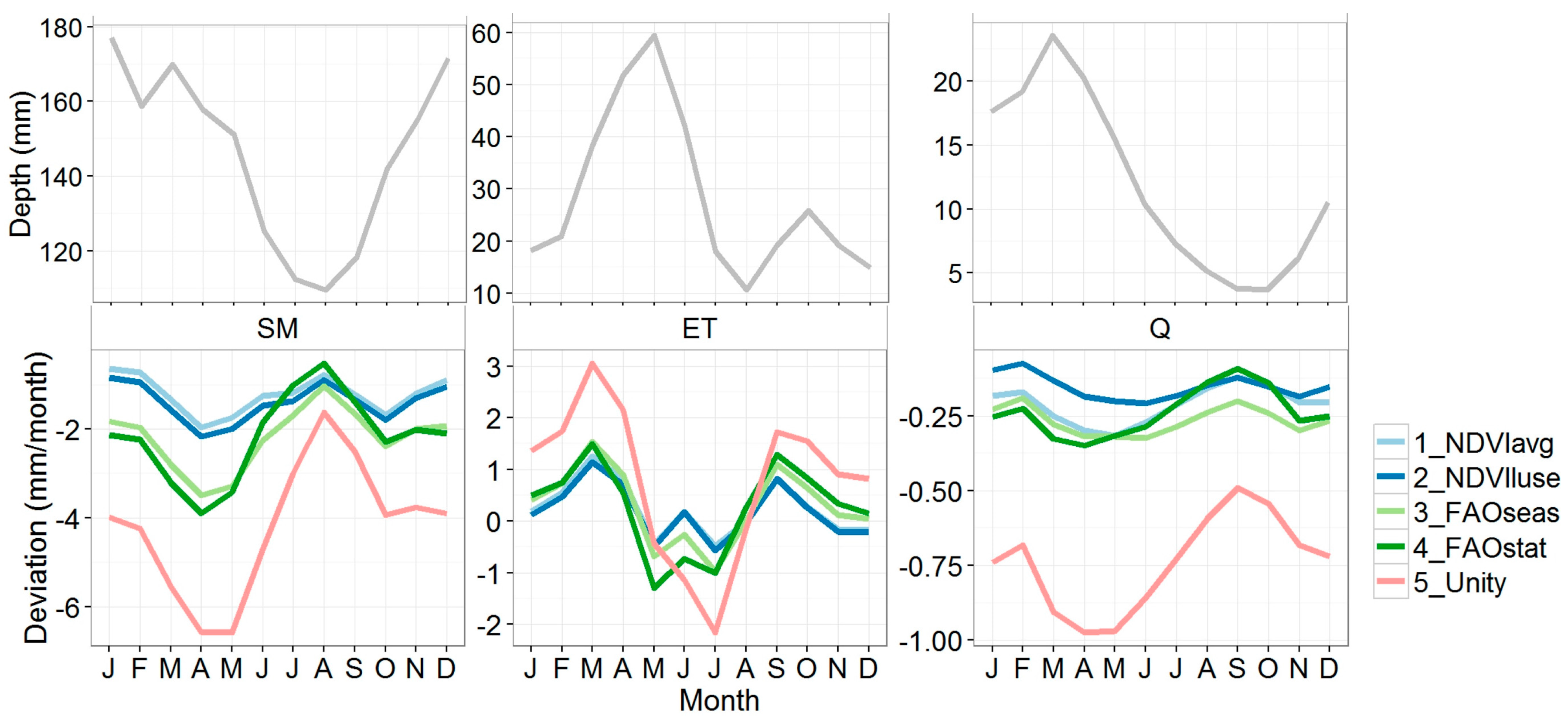
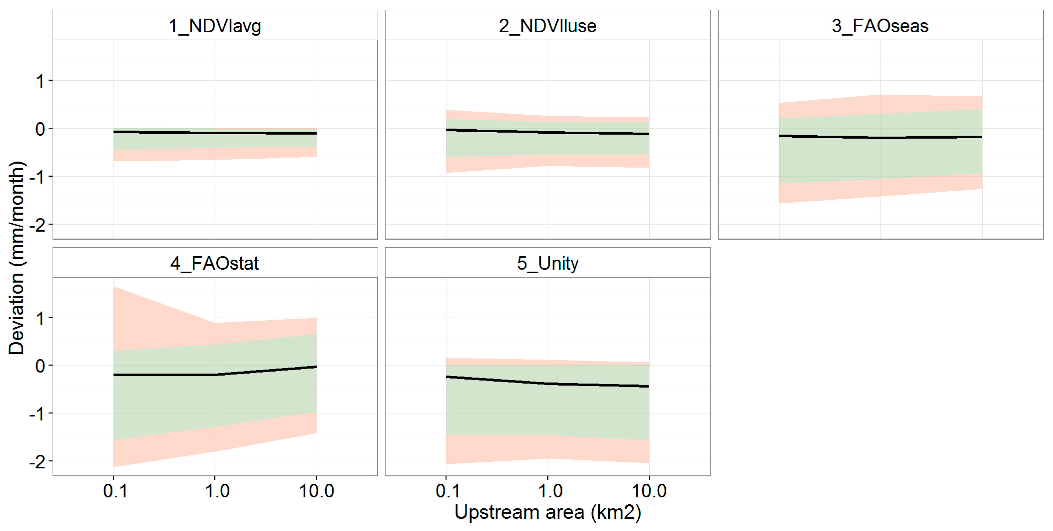
| Code | Data Source | Temporal Aggregation | Description |
|---|---|---|---|
| 0_NDVIref | NDVI (MODIS MOD13A1) | No aggregation, time series with maps each 16-days, 16 years (total 368 maps) | NDVI maps from MODIS product (gap-filled with monthly pixel mean value) |
| 1_NDVIavg | NDVI (MODIS MOD13A1) | Multi-year averages by each 16-day period (total 23 maps) | Pixel averages of 0_NDVIref, by each 16-day timestep and for 16 years |
| 2_NDVIluse | NDVI (MODIS MOD13A1), land use map | Multi-year averages by each 16-days period (total 23 maps) | Averages for each land cover type, calculated from 0_NDVIref, by each 16-day timestep for 16 years |
| 3_FAOseas | FAO-56, land use map | Monthly maps of kc per land use type (total 12 maps) | The annual kc pattern is based on standard FAO literature values per land use type. |
| 4_FAOstat | FAO-56, land use map | Constant per land use type (annual maximum) (total 1 map) | The maximum crop coefficient per land cover is assigned |
| 5_Unity | None | Crop coefficient = 1 (total 1 map) | A value of kc = 1 for entire basin |
| Period | NSE | PBIAS | RSR |
|---|---|---|---|
| Calibration (2001–2010) | 0.72 | 25 | 0.53 |
| Validation (2011–2015) | 0.63 | −20 | 0.60 |
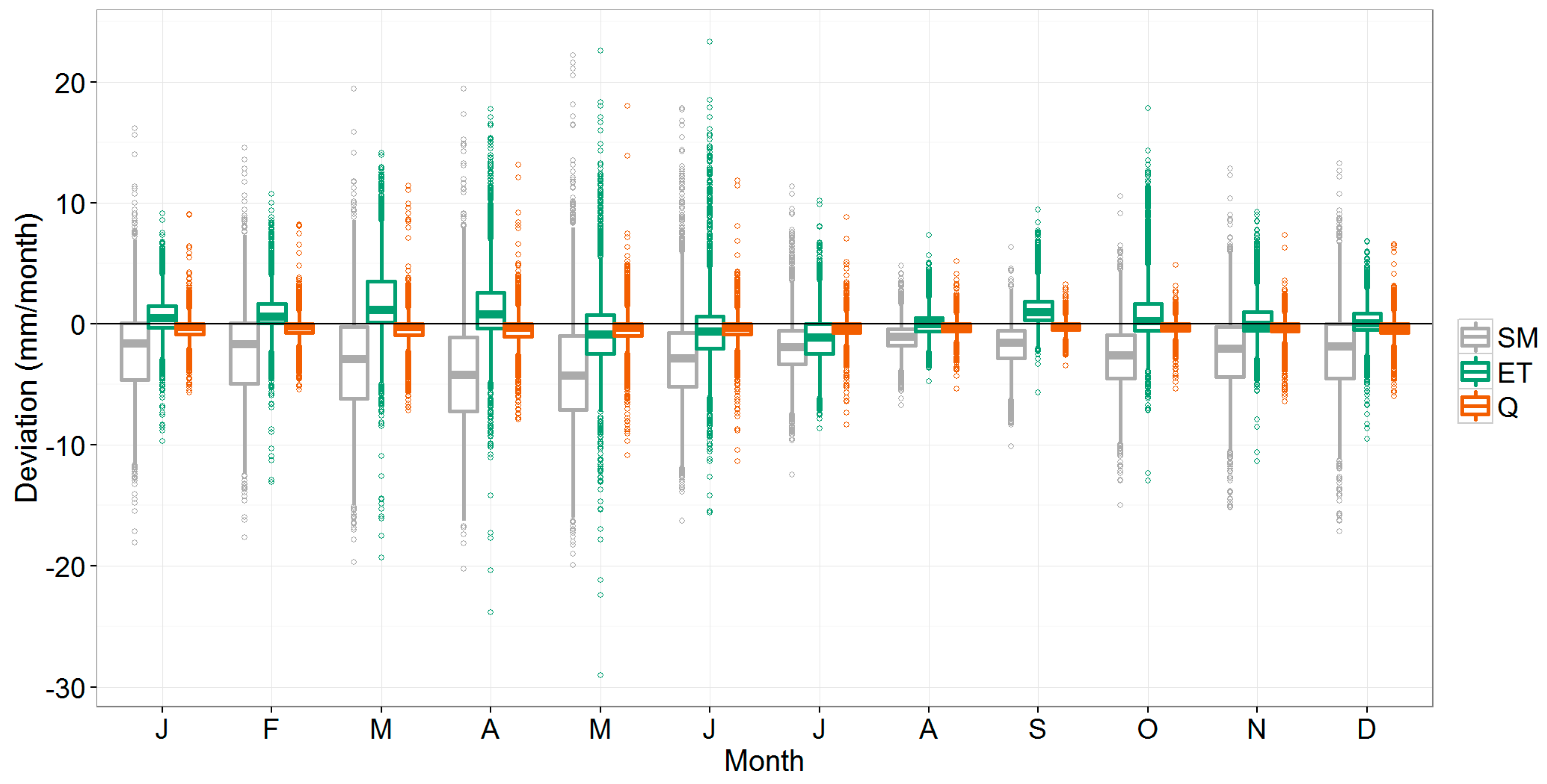
| Scale | Variable/Percentile | Absolute Deviations (mm/month) | Relative Deviations (%) | ||||
|---|---|---|---|---|---|---|---|
| 10th | 50th | 90th | 10th | 50th | 90th | ||
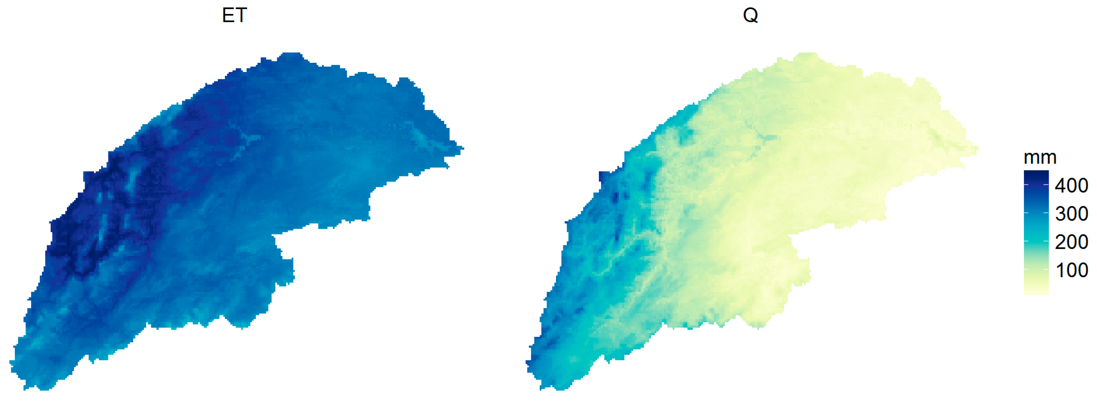
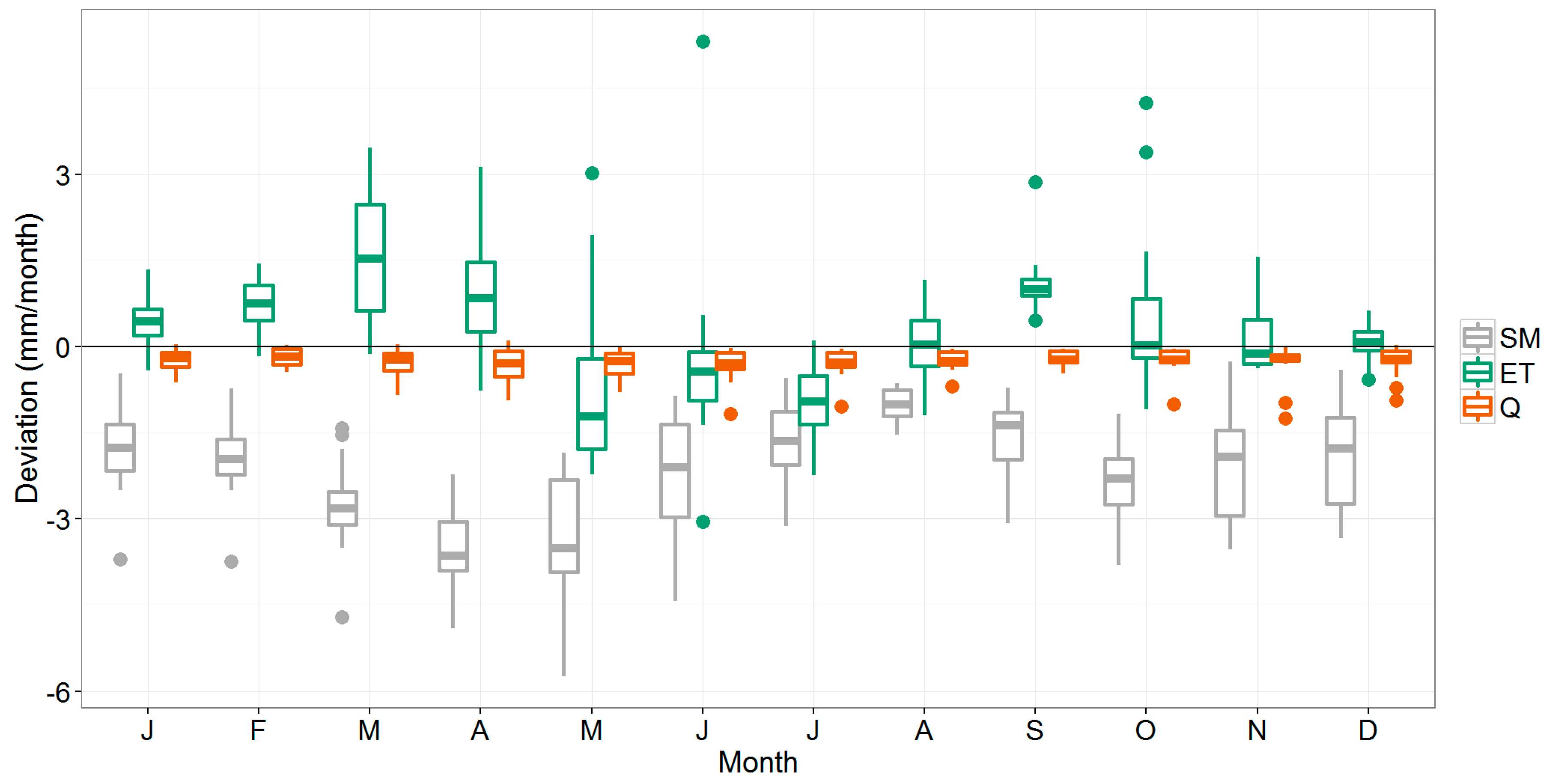
| Basin | SM | −3.6 | −2.0 | −1.0 | −2% | −1% | −1% |
| ET | −1.1 | 0.3 | 1.6 | −5% | 1% | 5% | |
| Q | −0.5 | −0.2 | 0.0 | −8% | −3% | 0% | |
| Sub-basins | SM | −7.3 | −2.1 | 1.3 | −5% | −2% | 1% |
| ET | −2.3 | 0.2 | 3.2 | −10% | 1% | 12% | |
| Q | −1.5 | −0.2 | 0.5 | −28% | −4% | 6% | |
© 2017 by the authors. Licensee MDPI, Basel, Switzerland. This article is an open access article distributed under the terms and conditions of the Creative Commons Attribution (CC BY) license ( http://creativecommons.org/licenses/by/4.0/).
Share and Cite
Hunink, J.E.; Eekhout, J.P.C.; Vente, J.D.; Contreras, S.; Droogers, P.; Baille, A. Hydrological Modelling using Satellite-Based Crop Coefficients: A Comparison of Methods at the Basin Scale. Remote Sens. 2017, 9, 174. https://0-doi-org.brum.beds.ac.uk/10.3390/rs9020174
Hunink JE, Eekhout JPC, Vente JD, Contreras S, Droogers P, Baille A. Hydrological Modelling using Satellite-Based Crop Coefficients: A Comparison of Methods at the Basin Scale. Remote Sensing. 2017; 9(2):174. https://0-doi-org.brum.beds.ac.uk/10.3390/rs9020174
Chicago/Turabian StyleHunink, Johannes E., Joris P. C. Eekhout, Joris De Vente, Sergio Contreras, Peter Droogers, and Alain Baille. 2017. "Hydrological Modelling using Satellite-Based Crop Coefficients: A Comparison of Methods at the Basin Scale" Remote Sensing 9, no. 2: 174. https://0-doi-org.brum.beds.ac.uk/10.3390/rs9020174