Wave Height Estimation from Shadowing Based on the Acquired X-Band Marine Radar Images in Coastal Area

Abstract

In this paper, the retrieving significant wave height from X-band marine radar images based on shadow statistics is investigated, since the retrieving accuracy can not be seriously affected by environmental factors and the method has the advantage of without any external reference to calibrate. However, the accuracy of the significant wave height estimated from the radar image acquired at the near-shore area is not ideal. To solve this problem, the effect of water depth is considered in the theoretical derivation of estimated wave height based on the sea surface slope. And then, an improved retrieving algorithm which is suitable for both in deep water area and shallow water area is developed. In addition, the radar data are sparsely processed in advance in order to achieve high quality edge image for the requirement of shadow statistic algorithm, since the high resolution radar images will lead to angle-blurred for the image edge detection and time-consuming in the estimation of sea surface slope. The data acquired from Pingtan Test Base in Fujian Province were used to verify the effectiveness of the proposed algorithm. The experimental results demonstrate that the improved method which takes into account the water depth is more efficient and effective and has better performance for retrieving significant wave height in the shallow water area, compared to the in situ buoy data as the ground truth and that of the existing shadow statistic method.

1. Introduction

As is well known, ocean wave is one of the most common ocean fluctuation phenomena. It is vitally important to understand the waves and their associated characteristics for ocean research and ocean exploitation [1,2,3,4]. Therefore, it is urgent to carry out all-round, multi-means and stereoscopic monitoring of the ocean. With the rapid development of computer and marine remote sensing techniques, it is becoming possibly to conduct the measurement of large area and real-time monitoring of the ocean by using X-band marine radar [5,6].

Nowadays, the X-band marine radar, which is commonly used to monitor moving vessels for its economy and popularity and has the capacity of observing the ocean surface with high spatial and temporal resolutions [5,6,7,8], also has been utilized widely to extract the wave spectrum and the variously statistical sea state parameters such as significant wave height, wave peak period, wave direction, bathymetry, sea surface elevation and sea surface currents from coastal areas or moving platforms [9,10,11,12,13,14,15,16]. The retrieving significant wave height from X-band marine radar images is one of the hot issues of ocean remote sensing in recent years. Currently, there are two different methods of extracting wave height, namely spectral analysis method and image shadow statistical method.

The basic idea of spectrum analysis method is to achieve the wavenumber energy spectrum of sea wave by using the three-dimensional discrete Fourier transform (3D DFT), and then to calculate the signal-to-noise ratio (SNR) of the wave signal. The significant wave height is estimated based on the empirical linear relationship between the significant wave height and the root mean square (RMS) of SNR. However, the coefficients of the linear relationship are closely related to radar characteristics and are commonly calibrated by using measured in situ buoy data. By taking into account the spatial and temporal variation characteristics of the sea clutter signal of X-band radar images, the 3D DFT was firstly utilized to obtain the wavenumber frequency image spectrum, which laid a foundation for using the SNR to measure wave height in practice [17]. The method to calculate the significant wave height based on SNR ratio was firstly proposed in [15] and the least squares (LS) method was used to fit the linear parameters. And the effectiveness of the method was verified compared to the in situ buoy data. An improved dispersion relation filter, which makes the wave spectrum estimated more accurate, was proposed in [18]. Meanwhile, the accuracy of the estimated wave height was improved. The geometric optics approximation principle was adopted to improve the empirical modulation transfer function (MTF) which changed the image spectrum to wave power spectrum. The accuracy of the estimated sea wave spectrum and the estimated significant wave height was further improved [19]. The spectral energy of background noise was applied to estimate the significant wave height by analyzing the definition of the SNR of sea wave [20]. The significant wave height is traditionally determined by utilizing the empirical linear relationship. However, the relationship is not completely linear, due to the effect of different calculation methods of SNR, environmental changes in the sea area, radar system differences and other factors in practice. Furthermore, an external equipment such as a buoy is demanded to calibrate the coefficients.

Fortunately, the shadow statistical method to estimate the significant wave height is not seriously affected by the above factors, and more attention has been attracted in recent years [14,21]. Moreover, this method has an enormous advantage and research value, since the external reference is not required for calibration. The physical modulation of the remote sensing image of ocean wave has significant characteristics in radar gray-level image statistic. Therefore, the significant wave height can be retrieved based on the shadow statistic of the radar image.

Assume the sea surface is a Gaussian surface, the backscattering model of the electromagnetic wave under the low incidence angle is analyzed by using the geometrical optics of the rough surface [22]. Thus, the radar image can be divided into bright and dark areas, and then, the wave height can be estimated by calculating the proportion of the bright area of the radar image. In order to solve the problem that the shadow method fails in high sea conditions, the segmenting gray-scale threshold method based on the normalized radar cross section (NRCS) was proposed [23]. The experimental results show that the modified method could improve the accuracy of the estimated wave height. With the increase of the shadow ratio under the high sea condition, Rune found that the variance of the differential gray image changes with the wave height based on the abundant experiments in [24]. Thus, the significant wave height could be determined by using this relation. In [25], the calculation deviation in [22] was analyzed by simulation experiment and the relationship between radial distance and threshold was discussed. In addition, it pointed that the gray threshold should be changed with the effective range of the radar. Under different polarizations, the dominant role of geometric and partial shadowing in shadowing modulation was discussed in [26]. The experimental results present that partial shadowing plays an important role on the shadowing modulation of sea clutter imaging, which provides the theoretical basis for retrieving the significant wave height based on the shadowing of radar images. In practice, it was difficult to distinguish whether the radar image is mainly modulated by geometric or partial shadowing, since the differences, which related to SNR, geometric factors and radar property, between the two shadowing were very small [14]. The significant wave height was achieved by combing the shadow image, which is extracted by a band-pass filter based on the edge detection, and the geometrical shadow theory of the random rough surface in [14]. The proposed algorithm successfully solved the difficult problem of shadow discrimination and could directly estimate the wave height without any external reference calibration. Due to the shadow statistical distribution of shadow images may be abrupt, a method to refine the threshold by smoothing the gray-scale intensity histogram was proposed in [21]. Moreover, the analyzing area of the radar image in the upwind direction is selected to retrieve the significant wave height. Based on the shadowing information and the support vector regression (SVR) algorithms, the significant wave height is estimated from marine radar images of the sea surface in [27]. Although the calibration is not necessary and high retrieving accuracy can be obtained, a large data set is required for training and the accuracy depends on the size of the data. According to the characteristic that the shadowing in the radar image changes with the distance from radar antenna to the sea surface, the method to estimate the significant wave height by using the visualization function was proposed in [28]. The feasibility of this method was proved by the simulated radar image. However, further research and validation are still needed in practice, since only the shadowing modulation was considered. Based on the theoretical analysis, it is found that the formula, which utilizes the wave slope to estimate the wave height in [14,21], is derived under the hypothesis of infinite deep water. For the sake of achieving more accurate wave height measurements, the strategy of a subarea selected along the upwind direction and smoothing the edge pixel intensity histogram is utilized. The experiment results show that the performance of the modified shadowing algorithm is better than the method based on SNR [29]. Commonly, the requirement of the deep water condition is not satisfied for the near-shore area. Although the significant wave height is directly estimated by using the existing wave slope formula in [14,21] from the radar images collected in the near-shore area, the performance of the retrieved wave height is not ideal, since the water depth was not considered.

In this paper, the effect of water depth is taken into account in the theoretical derivation of the retrieving formula of wave height. Our primary goal is to propose an improved algorithm, which is more suitable for estimating wave height both in the shallow water and deep water areas, based on the shadow statistics to efficiently and effectively retrieve the significant wave height. This paper is organized as follows: Section 2 presents the basic method to estimate the wave height based on the shadow statistics from the X-band radar image. The detailed theoretical derivation and the improved algorithm to retrieve significant wave height in the case of shallow water are developed in Section 3. In Section 4, the validity of the proposed method is investigated by the X-band radar images acquired. Finally, the conclusion is summarized in Section 5.

Notation: Scalars, vectors and matrices are expressed by regular, bold lowercase letters and bold uppercase letters, respectively.

2. The Estimation of Wave Height Based on the Shadow Statistics

With the development and progress of digital image processing technology, it is possible to estimate the significant wave height based on the shadow statistics of radar images when the electromagnetic wave is grazing into the sea surface. The method of shadow statistics not only successfully solves the problem of shadow discrimination, but also directly estimates the wave height without any external reference calibration [14,21]. Now we introduce the detailed description of the method for retrieving the significant wave height.

2.1. The Estimation of the Shadow Gray-Scale Threshold

Because of the modulation effect of the ocean wave imaging, the radar image is composed of bright and dark stripes. The significant wave height could be calculated based on the shadow statistics of the radar image. The premise of extracting the shadow image and calculating the shadow ratio of the radar image is to estimate the shadow threshold. By using the estimated shadow threshold, the radar image is divided into shadow area and the no shadow area, and then, the shadow ratio of the image can be obtained. The estimation of the shadow threshold based on X-band marine radar images is as follows:

2.1.1. The Shadow Edge Detection of the Radar Image

Edge images ${\mathbf{I}}_{Ei}(r,\theta )$ are obtained by convolving the original radar image $\mathbf{I}(r,\theta )$ with pixel difference operators in adjacent eight directions ${\mathbf{H}}_i(r,\theta )$, where $i\in \{1,2,\cdots ,8\}$, r and $\theta$ are the distance and the azimuth, respectively. For the sake of better filtering out noise, the edge value of the upper N-percentile of the edge image is selected as the threshold value. Thus, the thresholding of the edge image can be given by

$$\begin{array}{c}\hfill {\mathbf{I}}_{Ti}(r,\theta )=\left\{\begin{array}{cc}\hfill 1,& \hfill {\mathbf{I}}_{Ei}(r,\theta )>\mathrm{upper}N-\mathrm{percentile}\\ \hfill 0,& \hfill \mathrm{otherwise}\end{array}\right.\end{array}$$

(1)

where ${\mathbf{I}}_{Ti}(r,\theta )$ is the edge image after thresholding. And then, an edge image is obtained by superimposing the eight edge images extracted in eight different directions:

$$\begin{array}{c}\hfill {\mathbf{I}}_T(r,\theta )=\sum _{i=1}^8{\mathbf{I}}_{Ti}(r,\theta )\end{array}$$

(2)

2.1.2. The Elimination of the Isolated Noise Points

Based on the edge comparison method that each point in the edge image is compared with the threshold, the isolated noise point is removed. The specific formula is described as follows [14,21]:

$$\begin{array}{c}\hfill {\mathbf{I}}_F(r,\theta )=\left\{\begin{array}{cc}1,\hfill & \hfill {\mathbf{I}}_T(r,\theta )\in [1,{\tau }_F]\\ 0,\hfill & \hfill \mathrm{otherwise}\end{array}\right.\end{array}$$

(3)

where ${\tau }_F$ is the given threshold, ${\mathbf{I}}_F(r,\theta )$ is the edge image after filing out the isolated noise.

2.1.3. The Calculation of the Shadow Gray-Scale Threshold

For each value 1 of the edge image ${\mathbf{I}}_F$, the pixel value $\eta$ of the original radar image at the corresponding position can be found. Thus, a histogram function $F_H\left(\eta \right)$ of an edge image is established by the correspondence relationship between the edge image and the original radar image. The shadow gray-scale threshold ${\tau }_S$ is obtained by calculating the mode of the histogram function, which is shown below [14,21]:

$$\begin{array}{c}\hfill {\tau }_S=\mathrm{mode}\left(F_H\left(\eta \right)\right)\end{array}$$

(4)

where the mode function equals the largest number of occurrences.

2.2. The Calculation of the Illumination Ratio of the Radar Image

The original radar image $\mathbf{I}(r,\theta )$ is divided into the shadow area and no shadow area by using the obtained gray-scale threshold ${\tau }_S$. Thus, the shadow image ${\mathbf{I}}_S(r,\theta )$ is achieved, which is given by [14,21]

$$\begin{array}{c}\hfill {\mathbf{I}}_S(r,\theta )=\left\{\begin{array}{cc}1,\hfill & \hfill \mathbf{I}(r,\theta )<{\tau }_S\\ 0,\hfill & \hfill \mathrm{otherwise}\end{array}\right.\end{array}$$

(5)

The shadow image is divided into sectors in the azimuth direction. The illumination ratio function $S\left(\gamma \right)$, which is a function of grazing angle $\gamma$, is obtained by calculating the shadow ratio in each sector.

2.3. The Estimation of the Average RMS Wave Surface Slope

The sea surface illuminated by the electromagnetic wave is regarded as a two-dimensional random rough surface model, since the sea surface can be seen as the superposition of numerous individual cosine or sine waves with different directions, amplitudes, and initial phases. In order to facilitate the research, the two-dimensional random rough surface model is reduced to one-dimensional model [14]. According to the Smith’s fitting function, the RMS slope ${\sigma }_{RMS}$ can be estimated. Owing to the effect of the radar looking angles, wind direction, wave direction and submarine topography, the echo intensity of radar image in azimuth is different. As a result, the shadow distribution and the estimated slope of different sectors are different. For the sake of reducing the retrieving error, it is commonly to estimate the significant wave height with the averaged RMS slope. The averaged RMS slope ${\sigma }_{RMS}^A$ is obtained by averaging the estimated slope of each sector.

2.4. The Estimation of the Significant Wave Height

In practice, the commonly and currently used wave slope is as follows:

$$\begin{array}{c}\hfill {\sigma }_s=\frac{2\pi H_s}{g{T}_{m02}^2}\end{array}$$

(6)

where ${\sigma }_s$ is the significant slope, $H_s$ is the significant wave height, g is the gravity acceleration, $T_{m02}$ is the zero mean up-crossing wave period. Therefore, the relation between the significant wave height and the averaged RMS slope is given by [14,21]

$$\begin{array}{c}\hfill H_s=\frac{{\sigma }_{RMS}^{A}g{T}_{m02}^2}{\sqrt{2}\pi }\end{array}$$

(7)

3. The Improved Method for Retrieving the Significant Wave Height

3.1. The Definition of the Sea Surface Slope

The sea surface slope $\sigma$ of a periodic wave chain is generally defined as

$$\begin{array}{c}\hfill \sigma =\frac{H}{\lambda }\end{array}$$

(8)

where H is the wave height from the peak to the trough, $\lambda$ is the wavelength. In order to facilitate the engineering application and simplify the calculation, the wavelength is usually defined by other equivalent physical quantity, namely wave period, since the wavelength can not be measured directly. Thus, a new definition of sea surface slope is proposed by summarizing the existing research result. Under the condition of deep water and the first-order dispersion relationship, the sea surface slope can be rewritten as:

$$\begin{array}{c}\hfill \sigma =\frac{H}{\lambda }=H\frac{k}{2\pi }=\frac{H}{2\pi }\frac{{\omega }^2}{g}=\frac{H}{2\pi g}{\left(\frac{2\pi }{T}\right)}^2=\frac{2\pi H}{g{T}^2}\end{array}$$

(9)

where k is the wavenumber, $\omega$ is the the angular frequency and T is the wave period. The ideal dispersion relationship is used for the third equality. Here, it is observed that Equation (6) is achieved when the surface slope $\sigma$ and the wave height H in Equation (9) are replaced .

3.2. Retrieving the Significant Wave Height Based on the Sea Surface Slope in Near-Shore Area

Based on the theoretical analysis, it can be found that Equations (6) and (9) are derived under the assumption of infinite deep water, i.e., $d/\lambda \ge 0.5$, where d is the water depth. Therefore, Equation (6) is not suitable for retrieving wave height in the shallow water area. As a result, when the significant wave height is directly estimated using Equation (6), the accuracy will be seriously deteriorated. In this paper, the improved algorithm to retrieve the significant wave height based on the sea surface slope which is suitable for shallow water area is developed. The water depth is taken into account in the theoretical derivation of sea surface slope and retrieving significant wave height. The detailed derivation is given below:

When the surface current is ignored, the wave velocity c is given by

$$\begin{array}{c}\hfill c=\frac{\lambda }{T}=\frac{\omega }{k}=\sqrt{\frac{g}{k}tanh\left(kd\right)}\end{array}$$

(10)

The third equal equality is based on the ideal dispersion relationship. According to Equation (10), we have

$$\begin{array}{c}\hfill \sqrt{\frac{g}{k}tanh\left(kd\right)}=\frac{2\pi }{Tk}\end{array}$$

(11)

Then, the modulus of wavenumber k can be expressed as

$$\begin{array}{c}\hfill k=\frac{4{\pi }^2}{T^{2}gtanh\left(kd\right)}\end{array}$$

(12)

To combine Equations (10) and (12), we have

$$\begin{array}{c}\hfill c=\frac{\lambda }{T}=\frac{gT}{2\pi }tanh\left(kd\right)\end{array}$$

(13)

Then

$$\begin{array}{c}\hfill \lambda =\frac{g{T}^2}{2\pi }tanh\left(kd\right)\end{array}$$

(14)

Thus, the sea surface slope in the shallow water region can be written as

$$\begin{array}{c}\hfill \sigma =\frac{H}{\lambda }=\frac{2\pi H}{g{T}^2}·\frac{1}{tanh\left(kd\right)}\end{array}$$

(15)

Then, the significant wave height can be expressed as

$$\begin{array}{c}\hfill H_s=\sigma \frac{g{T}^2}{2\pi }tanh\left(kd\right)=\frac{{\sigma }_{RMS}^{A}g{T}_{m02}^2}{\sqrt{2}\pi }tanh\left(kd\right)\end{array}$$

(16)

In the condition of deep water, $tanh\left(kd\right)\approx 1$, Equations (15) and (16) are simplified to Equations (9) and (7), respectively.

For the case of very shallow water, i.e., $d/\lambda \le 0.05$ and $tanh\left(kd\right)\approx kd$, we have

$$\begin{array}{c}\hfill {\omega }^2=gktanh\left(kd\right)=gk·kd\end{array}$$

(17)

then

$$\begin{array}{c}\hfill c^2=gd\end{array}$$

(18)

Therefore, we have

$$\begin{array}{c}\hfill \lambda =\frac{g{T}^2}{2\pi }kd=T\frac{g}{2\pi }·\frac{2\pi }{\omega }kd=Tg\frac{k}{\omega }d=Tc=T\sqrt{gd}\end{array}$$

(19)

According to Equation (14), the first equality holds. The forth equality is based on Equations (10) and (17) . The fifth equality is based on Equation (18). Therefore, in the case of very shallow water area, the wave height is given by

$$\begin{array}{c}\hfill H=\sigma \lambda =\sigma T\sqrt{gd}=\sqrt{2}{\sigma }_{RMS}^{A}T\sqrt{gd}\end{array}$$

(20)

Therefore, the significant wave height estimated based on the RMS sea surface slope at different water depth areas is described as

$$\begin{array}{c}\hfill H_S=\left\{\begin{array}{cc}\hfill \frac{{\sigma }_{RMS}^{A}g{T}_{m02}^2}{\sqrt{2}\pi },& \hfill d/\lambda \ge 0.5\\ \hfill \frac{{\sigma }_{RMS}^{A}g{T}_{m02}^2}{\sqrt{2}\pi }tanh\left(kd\right),& \hfill 0.05\le d/\lambda \le 0.5\\ \hfill \sqrt{2}{\sigma }_{RMS}^A\sqrt{gd},& \hfill d/\lambda \le 0.05\end{array}\right.\end{array}$$

(21)

3.3. The Improved Method for Retrieving Wave Height Based on the Sea Surface Slope

For the sake of facilitating the engineering application, the term $tanh\left(kd\right)$ in Equations (16) and (21) should be related to wave period instead of wavelength or wavenumber. From Equation (10), we have

$$\begin{array}{c}\hfill tanh\left(kd\right)=\frac{{\omega }^2}{gk}\end{array}$$

(22)

It can be observed clearly that it is hard to express the function $tanh\left(kd\right)$ with wave period T when the water depth is considered. It is well known that $tanh\left(kd\right)\approx 1$ when $d/\lambda \ge 0.5$ and $tanh\left(kd\right)\approx kd$ when $d/\lambda \le 0.05$. Thus, we have the idea to approximately describe $tanh\left(kd\right)$ with liner relation function in $d/\lambda \in (0.05,0.5)$. And then, we achieve the endpoints $(0.05,kd)$ and $(0.5,1)$, where $kd=\frac{2\pi }{\lambda }d=\frac{\pi }{10}$ when $d/\lambda =0.05$. Based on the two endpoints, a liner function as the approximate function of the term $tanh\left(kd\right)$ can be obtained. However, a large error exists when the approximate linear function, which is directly obtained by water depth boundary conditions, is used to represent the function $tanh\left(kd\right)$.

To solve this problem, we choose the optimal endpoints by minimizing the root mean square error (RMSE) between the approximate piecewise function and the function $tanh\left(kd\right)$. Suppose that the left and right endpoints are $(x_1,kd)$ and $(x_2,1)$, respectively, where $kd=2*\pi x_1$ and $x_1<x_2$, by minimizing the RMSE, we have

$$\begin{array}{c}\hfill x_1=0.098,x_2=0.289\end{array}$$

(23)

Thus, we use the calculated endpoint value to construct the approximate function $tanh\left(kd\right)$. As shown in Figure 1, the red solid line and the blue dash line denote the approximate function by minimizing the RMSE and the function $tanh\left(kd\right)$, respectively. The constructed approximate function is shown as

$$\begin{array}{c}\hfill tanh\left(kd\right)=2.0118\frac{d}{\lambda }+0.4186=0.3202kd+0.4186\end{array}$$

(24)

Here, it is observed clearly that the constructed piecewise function is pretty close to the function $tanh\left(kd\right)$. In addition, it also shows that Equation (7) which neglects the effect of water depth will seriously affect the retrieving accuracy of wave height in the shallow water area. In the ideal case of infinite water depth, $tanh\left(kd\right)\approx 1$. For our designed approximate function, although the fitting error exists, it is much smaller than that of $tanh\left(kd\right)\approx 1$. To combine Equations (22) and (24), and then we achieve

$$\begin{array}{c}\hfill 0.3202d{k}^2+0.418k-\frac{4.0284}{T^2}=0\end{array}$$

(25)

Because k is the modulus of wavenumber, k is always positive for any d and T. Thus, we select the solution of positive wavenumber and have

$$\begin{array}{c}\hfill k=\frac{-0.418+\sqrt{0.1747+\frac{5.1596}{T^2}d}}{0.6404d}\end{array}$$

(26)

To substitute the achieved wavenumber k into Equation (24), we can obtain

$$\begin{array}{c}\hfill tanh\left(kd\right)=\sqrt{0.0437+1.2899\frac{d}{T^2}}+0.2096\end{array}$$

(27)

Suppose $T=T_{m02}$, Equation (21) can be rewritten as

$$\begin{array}{c}\hfill H_S=\left\{\begin{array}{cc}\hfill \frac{{\sigma }_{RMS}^{A}g{T}_{m02}^2}{\sqrt{2}\pi },& \hfill d/\lambda \ge x_2\\ \hfill \frac{{\sigma }_{RMS}^{A}g{T}_{m02}^2}{\sqrt{2}\pi }(\sqrt{0.0437+1.2899\frac{d}{T^2}}+0.2096),& \hfill x_1\le d/\lambda \le x_2\\ \hfill \sqrt{2}{\sigma }_{RMS}^A\sqrt{gd},& \hfill d/\lambda \le x_1\end{array}\right.\end{array}$$

(28)

4. The Results and Analysis of the Experiment

In this section, we carry out retrieving the significant wave height based on the collected radar images at a near-shore area to examine the validity of our proposed method. Also, the detailed experiment site and field data are described. In order to simplify the computing time and improve the accuracy of edge detection, the radar images are sparsely processed before utilized to retrieve significant wave height in this paper. The performance of our modified method for retrieving wave height is presented by comparing with that of the existing shadow statistical method and the in situ buoy data.

4.1. Field Data

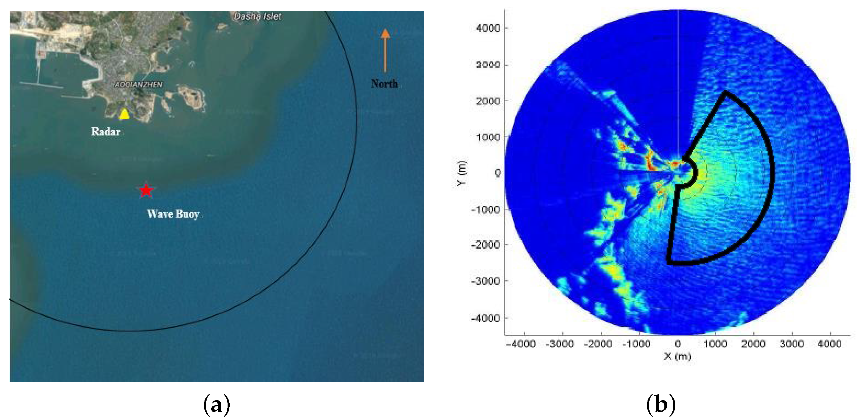
To examine the validity and effectiveness of the developed algorithm, the data collected at Pingtan which locates at Haitan island of Fujian province from October to November in 2010 were applied for analysis. In addition, a large data set collected at Pingtan from November 2014 to January 2015 is also applied to certify the effectiveness of our proposed method. The radar parameters for the two different test data sets are same. The RM-1290 marine radar is used to acquire radar images. The parameters of the X-band marine radar are shown in

Table 1. The parameters of X-band marine radar.

Radar Parameters	Value
Electromagnetic Wave Frequency	9.3 GHz
Antenna height	45 m
Antenna rotation speed	22 r.p.m
Antenna Gain	31 dB
Polarization	HH
Antenna length	1.8 m
Horizontal Beam Width	0.9${}^{\circ }$
Vertical Beam Width	21${}^{\circ }$
Pulse Repetition Frequency	1300 Hz
Pulse Width	50 ns

. Also, a wave buoy is deployed to measure the wave height as the ground truth. The sampling frequency of wave buoy is 2 Hz. The site of radar and wave buoy is shown in Figure 2a. The average water depth at this area is about 28 m. Since the accurate terrain data in this area is not obtained, the average water depth is used in the processing without considering the variation effect of water depth. The buoy is deployed at about 800 m from the radar. The water depth at the buoy location is about 25 m. The installed location of radar is 25${}^{\circ }$20${}^{\prime }$N 120${}^{\circ }$08${}^{\prime }$E. The radar image covers a radius of about 0.5∼4.3 km and works in short pulse mode. The acquisition card of 60 MHz high sample rate is chosen in the data acquired system for the sake of acquisition signal without distortion. After acquisition processing with a 14-bit digital acquisition card, the echo intensity is mapped to 0∼8191. In order to facilitate the subsequent experimental processing, the radar echo intensity is mapped to 0∼5000, since the signal with the value greater than 5000 is few and mainly noise. The original image acquired using the X-band marine radar is shown in Figure 2b. The radial resolution of the radar image is 7.5 m, and the azimuthal resolution is ${0.1}^{\circ }$. There are 600 sampling points in the distance direction. The left part of Figure 2b is the echo area of the land. The right part is the echo area of the sea surface which is the sea clutter. The echo area of the sea surface in the radar image is the effective echo region. During the experiment, the wind speed is great than 10 m/s, and the range of wave height is 2∼3 m.

The shadow statistical methods in this paper output a set of experimental result every 4 min, but the wave buoy which works only 20 min during 1 h outputs one set of experimental result every 1 h. In order to minimize the errors caused by inconsistent output time of different measuring methods, the outputs of the shadow statistical methods are averaged every 20 min, and then the retrieved significant wave height is compared with that of the buoy at the same working time. Thus, the experimental results are compared every 1 h. In addition, for the sake of decreasing the experimental error, the measured cross-zero period of the buoy is chosen for the shadow statistical methods in the experiment.

4.2. The Sparse Processing of Radar Image

The marine radar works on the rotation mode when scanning the sea surface. Thus, the marine radar image contains two-dimensional coordinate information of the distance and azimuth. Commonly, the acquired radar images have high azimuth resolution. Due to the swing influence of installation platform, the backscatter signal loss exists, which results that the line number of each radar image is not fixed. If the significant wave height is directly performed using the raw radar image, it will lead to the following two questions: First, because of a large amount of radar data, it consumes much time to perform image edge detection and estimate the sea surface slope in the follow-up. Second, it results in the edge blurring in azimuth owing to the uneven distribution of radar echo in azimuth and the high azimuthal resolution, which is not conducive to edge detection.

Based on the above analysis, it is necessary to dilute the radar image in azimuth so that the radar image is uniformly distributed in azimuth and the difference between any two adjacent lines becomes larger which are benefit to the edge detection of the radar image. Meanwhile, the amount of image data is correspondingly reduced, and it can improve the efficiency of edge detection and the speed of operation.

4.3. Experimental Results and Analysis

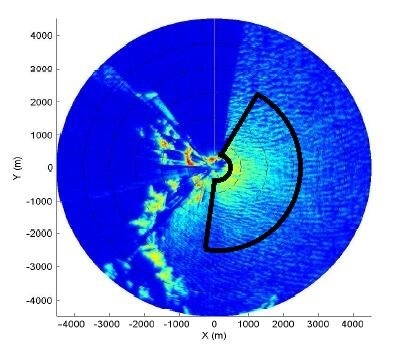
The effective echo region in back sector area of Figure 2b is selected to carry out retrieving the significant wave height. In addition, the radar images are preprocessed to suppress the co-frequency interference [30] and identify the rain and snow noise [31] before utilized to retrieving wave height. Since the radar echo intensity is saturated and the radar echo are mainly affected by the tilt modulation in the near segment of the radar image, the selected area is at least 400 m from the radar platform. In addition, as the radar echo intensity decreases with the increase of radius, when it is too far away from the radar antenna, the radar can not receive sea clutter signal which completely buries in the system noise. Moreover, it is significantly important to select the effective echo area as large as possible in azimuth so as to improve the estimation accuracy of the wave height. The grazing angle corresponding to the radar image data is generally distributed in the range of 1∼10${}^{\circ }$. Combining with the texture features of radar image, the sector analysis area in the range of 400∼2500 m without obstructions and fixations are selected to retrieve the significant wave height. In this case, the radar images selected are mainly modulated by shadowing. The selected analysis area of radar image in Cartesian coordinate system is shown in Figure 3. In practice, since the height of the radar antenna may be different, it is necessary to select the image region that the shadowing dominates the main modulation mechanism under the same grazing angle.

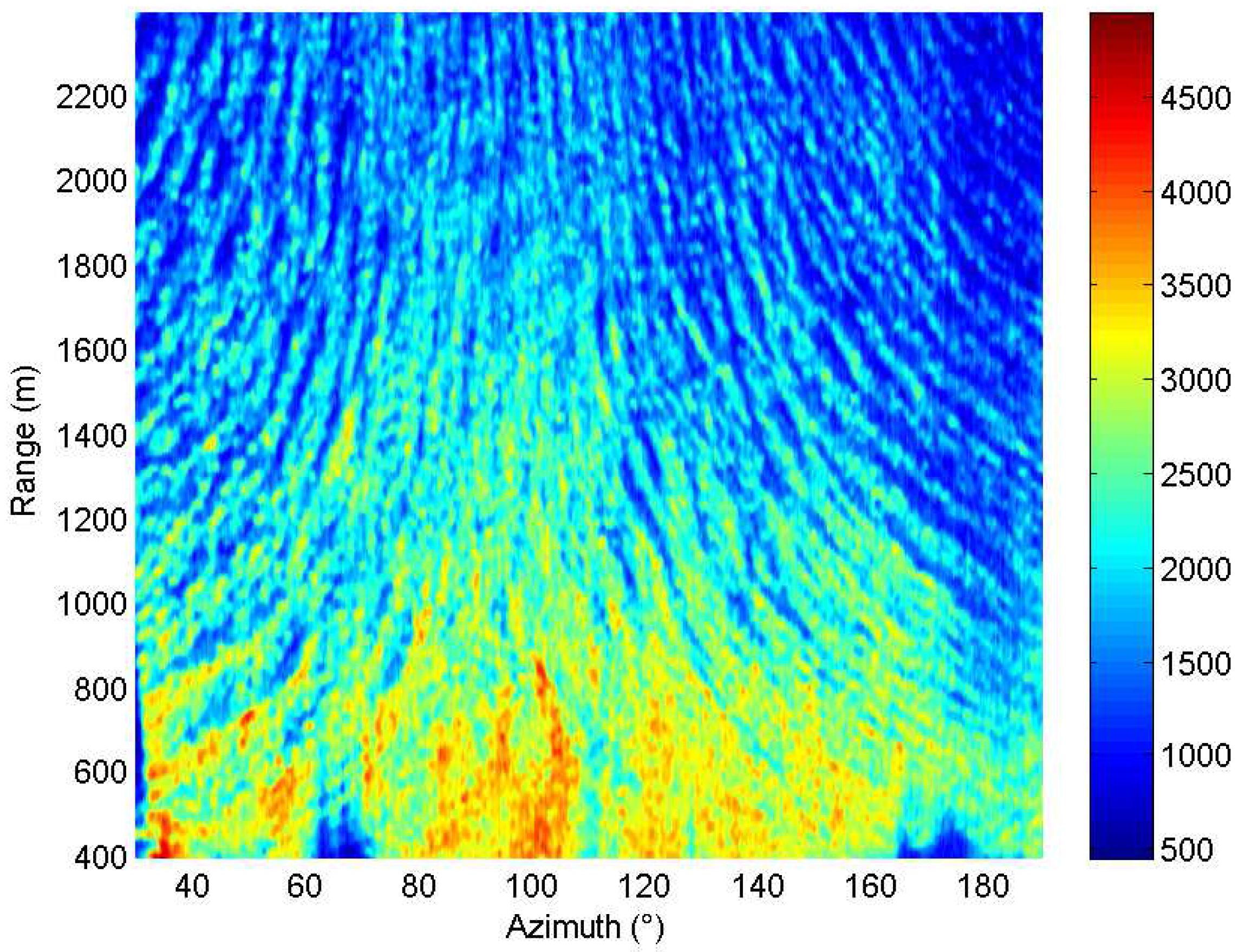
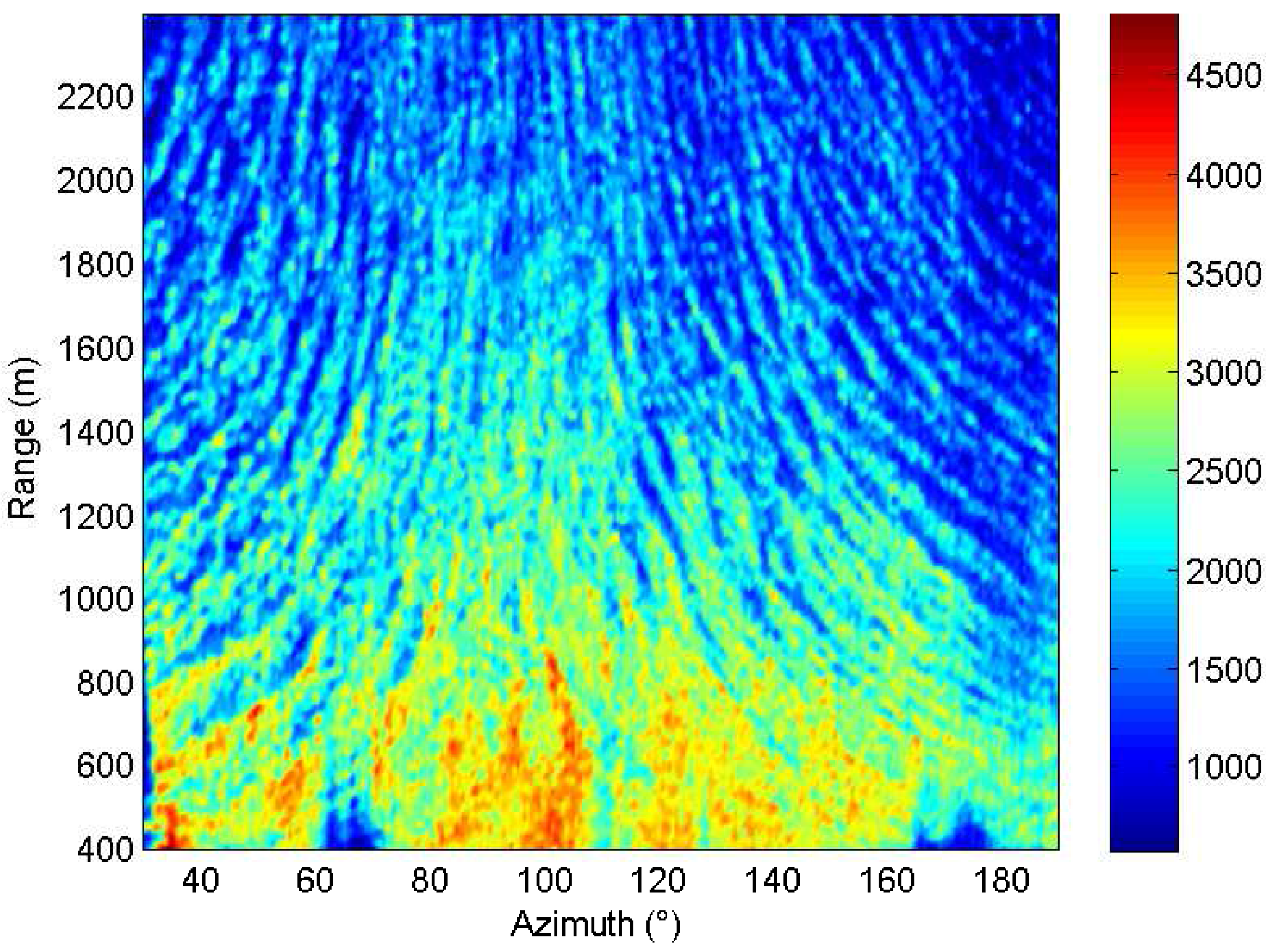
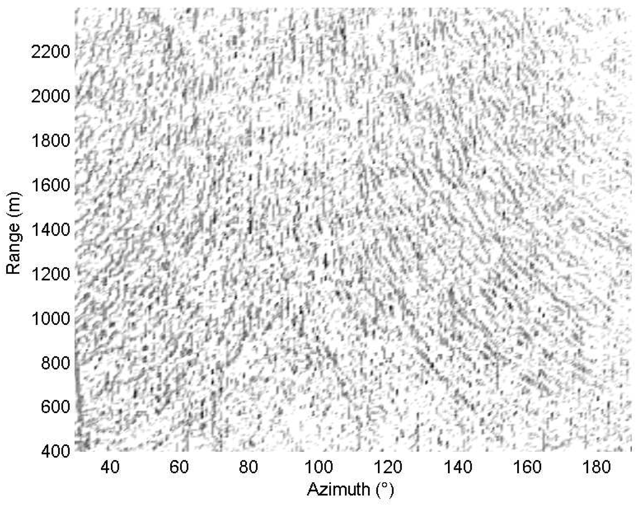
The angular resolution of the original radar image is higher and the pixel gray level changes smoothly in azimuth, which is not good for image edge detection. Therefore, it is necessary to perform a thinning process before retrieving the wave height. If the number of lines in the selected analysis area is too much and the amount of data is too large after the thinning processing, the subsequent processing will be cumbersome. On the contrary, lots of useful wave information will be lost, and the persuasion is poor. After the comprehensive evaluation and experimental study, it is found that the performance of the retrieved wave height is best when the azimuth resolution is reduced to ${0.6}^{\circ }$. Figure 4 shows the radar image after sparse processing of Figure 3.

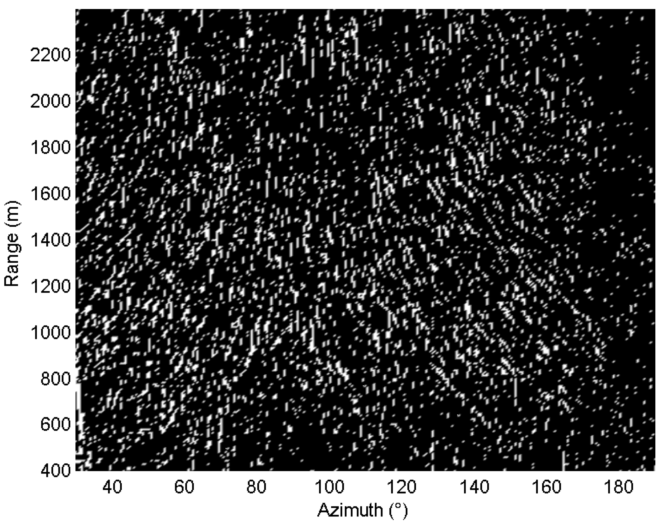
It can be seen that Figure 4 not only preserves the basic texture feature of the sea wave, but also enhances the difference between the image pixels which facilitates the subsequent edge detection. Now, the pre-processed radar image can be utilized for image edge detection. The directional edge image is obtained by convolving the radar image pixels with the simple difference operator in eight directions. Then, the edge image which is achieved by superimposing the eight directional edge images is shown in Figure 5. The upper 10 percentile of the edge image is taken as the threshold [14,21]. And then, the obtained edge image after thresholding is shown in Figure 6. The edge of the sea clutter in Figure 6 can be observed clearly, where the black and white represent the value 8 and 1, respectively.

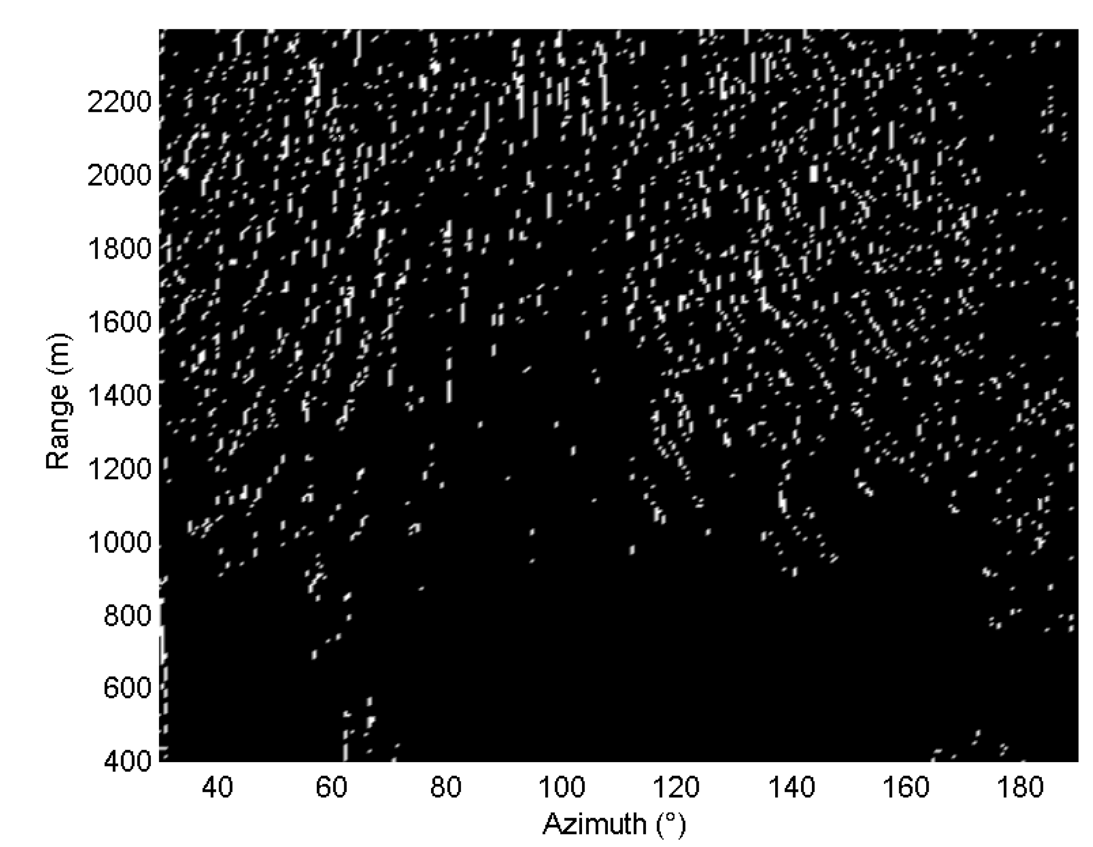
The threshold ${\tau }_F=6$ is used to remove the isolated noise [14,21]. Actually, the pixels ${\tau }_F>6$ may also belong to a small shadow, but ignoring these points will not cause the loss of valid information. The edge image after thresholding and filtering is shown in Figure 7. Thus, the image edge of the marine radar is determined.

The corresponding pixels of the edge image in the radar image is used to perform a histogram statistics. Then, the shadow gray-scale threshold ${\tau }_S$ is obtained by taking a mode on the histogram. The histogram statistics and the gray-scale threshold which are respectively indicated by the pink curve and red vertical dotted line are shown in Figure 8. In addition, the histogram of the radar image is also presented. The blue curve is the overall gray-scale distribution curve of the radar image.

From Figure 8, it can be observed clearly that the threshold obtained by direct taking mode on the histogram statistics of the radar image is different from the shadow gray-level threshold ${\tau }_S$. This difference also reflects the non-linear imaging characteristics of the marine radar image and the modulation effects on the radar imaging. The process to select the shadow gray-scale threshold for retrieving the wave height in the shadow statistical method is similar to the process to transfer the image spectrum to wave spectrum with the experimental MTF in the 3D DFT method.

Now, the radar image can be divided into shadow and no shadow areas by using the obtained shadow gray-scale threshold ${\tau }_S$. The shadow image of the radar image collected is shown in Figure 9, where threshold ${\tau }_S=1500$. The bright part indicates the shadow area shaded by high ocean waves, and the black part indicates the waves observed by the radar. The texture features of the waves can be clearly observed. As the distance from the radar antenna increases, the image shadow gradually increases.

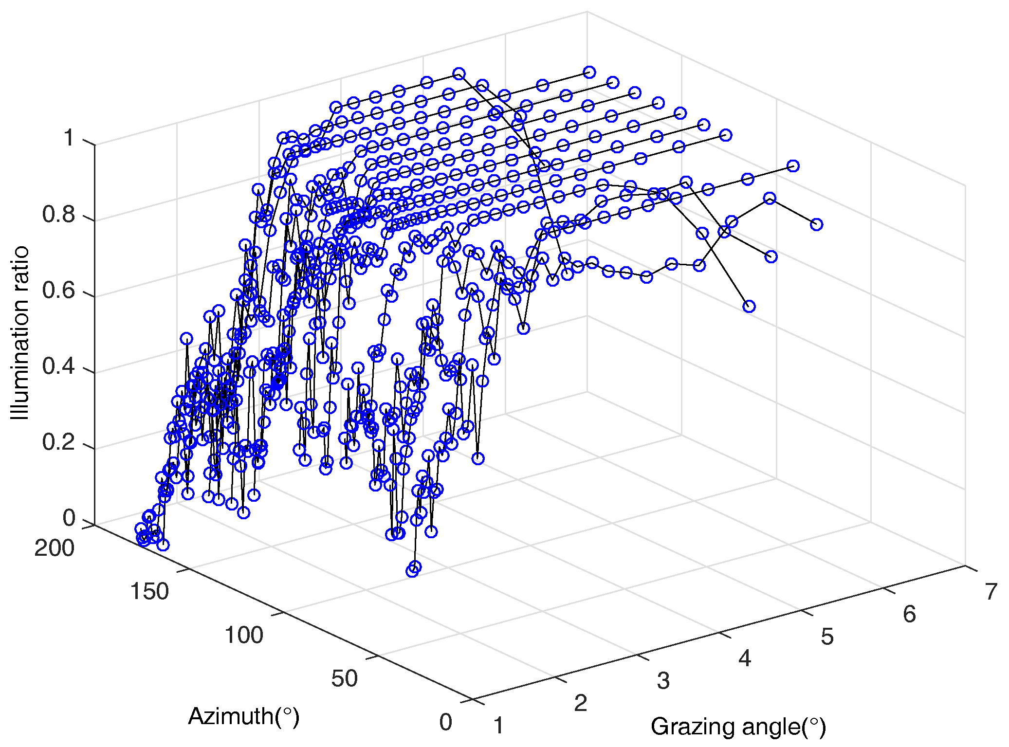
In order to calculate accurately the shadow ratio in the shadow image which is a function of relating to the grazing angle, commonly, the shadow image every ${10}^{\circ }$ in azimuth is divided into a sector. And then, each partition in the radial distance is divided into 30∼50 blocks so that each block corresponds to different grazing angle. Thus, the shadow ratio of each sector under different grazing angle is obtained. Based on the shadow ratio function, the illumination curve in different sector is achieved, which is shown in Figure 10.

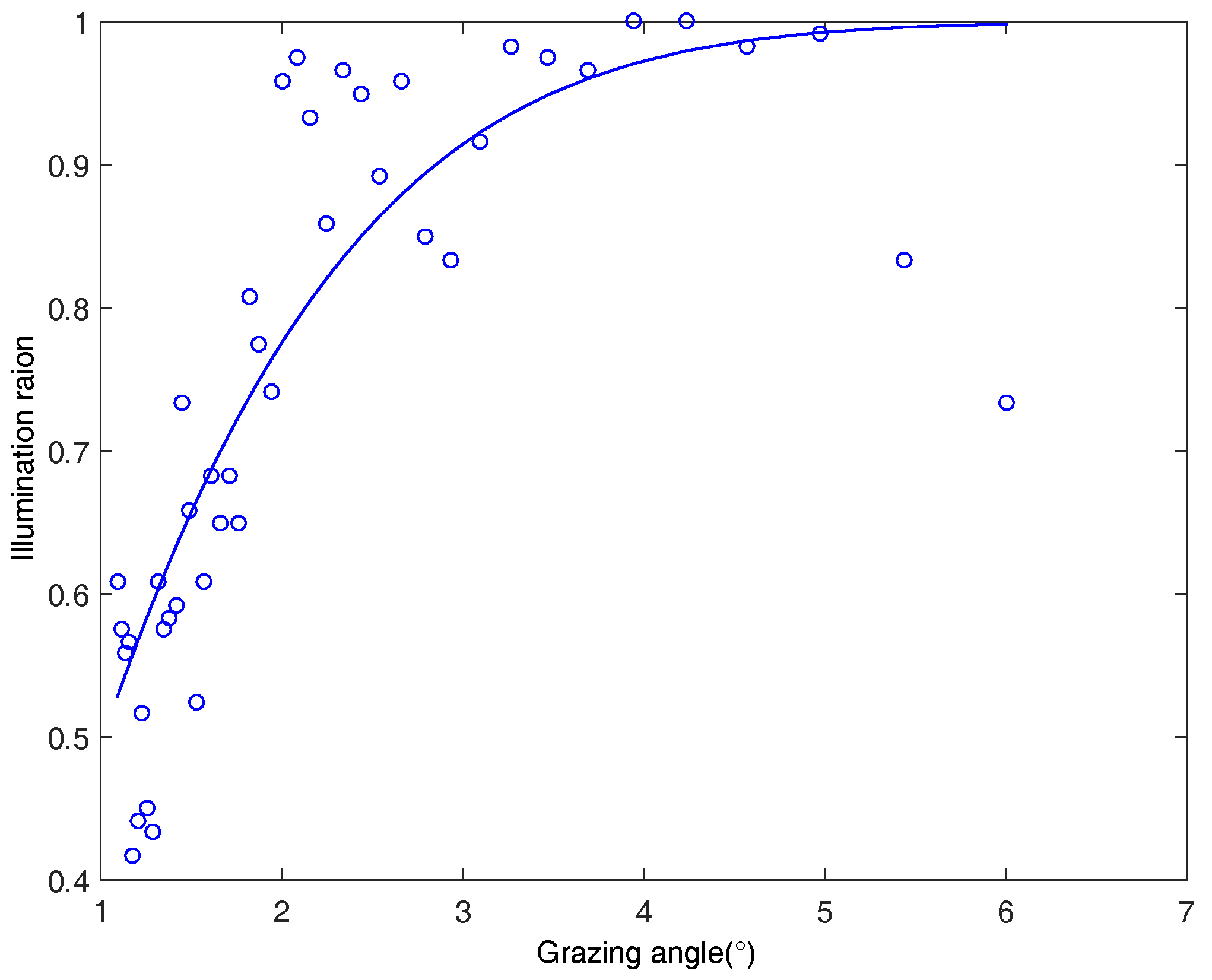
For one sector in azimuth, the calculated illumination as a function of grazing angle and the fitted Smith’s function are shown in Figure 11. The blue circle represents the illumination probability obtained, and the blue curve denotes the fitted Smith’s function. In order to avoid the influence of the far-near effect on the retrieving wave height, the illumination with the grazing angle less than $1^{\circ }$ is not taken into account in the subsequent processing.

Figure 12 is the estimated RMS sea surface slope on each sector by fitting the Smith’s function. From Figure 12, it can be seen that the estimated sea surface slope in each sector is different. Therefore, in order to reduce the influence of the slope on the retrieving accuracy, the average RMS by averaging the obtained RMS at different sectors is utilized.

The estimated significant wave height from X-band marine radar images and the buoy record in situ during the experiment are illuminated in Figure 13. Based on the acquired radar images in the near-shore area, it can be observed that the estimated wave height based on the modified method is closer to the reference value than that of the traditional shadow statistical method. And, the retrieved wave height based on the modified method is smaller than that of the traditional method, since the function term $tanh\left(kd\right)$ is smaller 1 and is taken into account in the modified method.

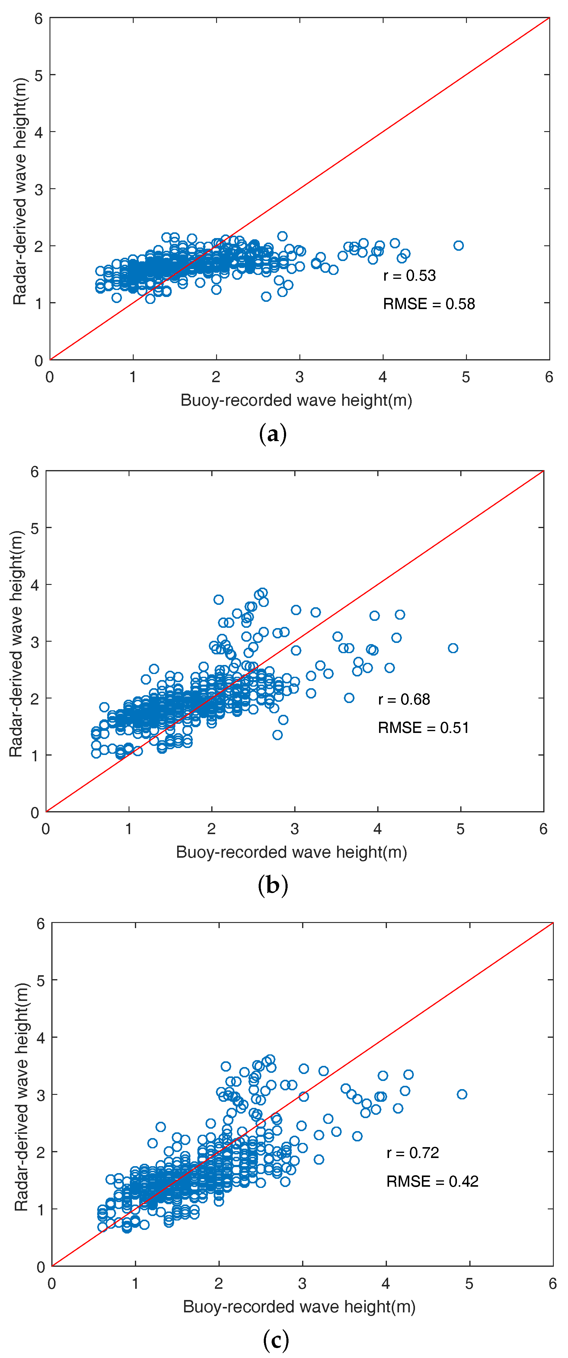
To further verify the effectiveness of the improved algorithm, the scatter plots between the radar-retrieved wave height and the buoy-retrieved wave height are presented in Figure 14. Figure 14a shows the scatter plot between the radar-retrieved wave height based on the SVR method and the buoy-retrieved wave height in the near-shore area. The SVR method can perform well after a successful training process in [27]. Since the dataset is not sufficient for training, the performance of the SVM method is not fully represented in our experiment. Figure 14b shows the scatter plot between the radar-retrieved wave height based on Equation (7) and the buoy-retrieved wave height in the near-shore area. Figure 14c shows the scatter plot between radar-retrieved wave height based on Equation (28), which considers the water depth, and the buoy-retrieved wave height. From Figure 14, it can be observed clearly that our improved method has a relatively better performance than the SVR method and the traditional method in the coastal area. The scatter distribution in Figure 14b is relatively scattered and the overall distribution is high, but the scattered distribution in Figure 14c is relatively more concentrated. The correlation coefficient between the wave height measured by the improved algorithm and the external reference is 0.72, which is larger than that of the traditional algorithm. The RMSE of the traditional algorithm is 0.51, but the RMSE of the improved algorithm is 0.42. Commonly, the improved algorithm works in shallow water since $x_1\le d/\lambda \le x_2$. In the case of high sea conditions, the improved algorithm works in very shallow water when $d/\lambda \le x_x$ as the wavelength increases. However, the traditional shadow statistic method works under the assumption of infinite deep water. Thus, the correlation coefficients of the improved algorithm is improved.

The comparison shows that the RMSE of the improved algorithm is much smaller than that of the traditional shadow statistical method. Compared with the traditional algorithm, the effectiveness of the improved wave height estimation algorithm based on the sea surface slope is verified. The experimental results certify that the modified method which takes into account the effect of the water depth on retrieving significant wave height can improve the retrieving accuracy in the shallow water area.

5. Conclusions

In this paper, the method to retrieve the significant wave height from X-band marine radar images based on shadow statistics is investigated, due to its advantage that any external reference is not required. Currently, the existing shadow statistical method is only applicable to the infinite water depth environment. Thus, the improved retrieving method in the shallow water area is carried out. The detailed analysis and derivation are presented. As a result, the improved method of retrieving wave height is applicable to both the deep water area and shallow water area. In addition, since the radar image collected by X-band marine radar distributes unevenly in azimuth and has high azimuthal resolution, it will lead to angle-blurred for the image edge detection and time-consuming in the estimation of sea surface slope. Therefore, the radar image is sparsely processed in advance for retrieving wave height. The validation of the proposed method is investigated by the acquired radar images in near-shore area. The experimental results have demonstrated that it is more accurate to extract wave height based on the improved method than that of the existing shadow statistical method.

However, the retrieving accuracy is still needed to improve for the application in practice. And, more experiments are required to verify the accuracy in various sea conditions. Owing to the effect of the angle between the looking direction of the radar and the upwind direction of the sea surface, the echo intensity of sea clutter in different azimuth, which may reduce the retrieving accuracy, is different. However, the research results on the echo intensity adjustment in the azimuth are still relatively rare. The radar echo intensity in different azimuth is different, which will lead to the great difference of the estimated RMS sea surface slope. Therefore, it is important to study the relationship between the RMS and the wind direction, and further consider the applicability of the algorithm under different sea conditions, wind speed and wave direction. In addition, the sea surface current is introduced to improve the retrieving accuracy of the shadow statical method, which is under our future investigation.

References

- Chen, Z.; Pan, J.; He, Y.; Devlin, A. Estimate of tidal constituents in nearshore waters using X-band marine radar image sequences. IEEE Trans Geosci. Remote Sens. 2016, 54, 6700–6711. [Google Scholar] [CrossRef]
- Chen, Z.; He, Y.; Zhang, B.; Qiu, Z. Determination of nearshore sea surface wind vector from marine X-band radar images. Ocean Eng. 2015, 96, 79–85. [Google Scholar] [CrossRef]
- Wei, Y.; Zhang, J.-K.; Lu, Z. A novel successive cancellation method to retrieve sea wave components from spatio-temporal remote sensing image sequences. Remote Sens. 2016, 8, 607. [Google Scholar] [CrossRef]
- Wei, Y.; Lu, Z.; Huang, Y. Wave parameters inversion from X-band marine radar image sequence based on the novel dispersion relation band-pass filter on the moving platform. J. Comput. Theor. Nanosci. 2016, 13, 5470–5477. [Google Scholar] [CrossRef]
- Dankert, H.; Horstmann, J.; Rosenthal, W. Wind- and wave-field measurements using marine X-band radar-image sequences. J. Ocean. Eng. 2005, 30, 534–542. [Google Scholar] [CrossRef]
- Huang, W.; Gill, E.; An, J. Iterative least-squares-based wave measurement using X-band nautical radar. IET Radar Sonar Navig. 2014, 8, 853–863. [Google Scholar] [CrossRef]
- Serafino, F.; Lugni, C.; Soldovie, F. A novel strategy for the surface current determination from marine X-band radar data. IEEE Geosci. Remote Sens. Lett. 2010, 7, 231–235. [Google Scholar] [CrossRef]
- Shao, W.; Li, X.; Sun, J. Ocean wave parameters retrieval from TerraSAR-X images validated against buoy measurements and model results. Remote Sens. 2015, 7, 12815–12828. [Google Scholar] [CrossRef]
- Dankert, H.; Rosenthal, W. Ocean surface determination from X-band radar-image sequences. J. Geophys. Res. 2004, 109. [Google Scholar] [CrossRef]
- Shen, C.; Huang, W.; Gill, E.W.; Carrasco, R.; Horstmann, J. An algorithm for surface current retrieval from X-band marine radar images. Remote Sens. 2015, 7, 7753–7767. [Google Scholar] [CrossRef] [Green Version]
- An, J.; Huang, W.; Gill, E.W. A self-adaptive wavelet-based algorithm for wave measurement using nautical radar. IEEE Trans. Geosci. Remote Sens. 2015, 53, 567–577. [Google Scholar]
- Senet, C.; Seemann, J.; Ziemer, F. The near-surface current velocity determined from image sequences of the sea surface. IEEE Trans. Geosci. Remote Sens. 2001, 39, 492–505. [Google Scholar] [CrossRef]
- Chuang, L.Z.-H.; Wu, L.-C. Study of wave group velocity estimation from inhomogeneous sea-surface image sequences by spatiotemporal continuous wavelet transform. IEEE J. Ocean. Eng. 2014, 39, 444–457. [Google Scholar] [CrossRef]
- Gangeskar, R. An algorithm for estimation of wave height from shadowing in X-band radar sea surface images. IEEE Trans. Geosci. Remote Sens. 2014, 52, 3373–3381. [Google Scholar] [CrossRef]
- Nieto-Borge, J.C.; Guedes Soares, C. Analysis of directional wave fields using X-band navigation radar. Coast. Eng. 2000, 40, 375–391. [Google Scholar] [CrossRef]
- Ludeno, G.; Reale, F.; Dentale, F.; Carratelli, E.P.; Natale, A.; Soldovieri, F.; Serafino, F. An X-band radar system for bathymetry and wave field analysis in a harbour area. Sensors 2015, 15, 1691–1707. [Google Scholar] [CrossRef] [PubMed]
- Young, I.; Rosenthal, W.; Ziemer, F. A three dimensional analysis of marine radar images for the determination of ocean wave directionality and surface currents. J. Geophys. Res. 1985, 90, 142–149. [Google Scholar] [CrossRef]
- Gangeskar, R. Ocean current estimated from X-band radar sea surface images. IEEE Trans. Geosci. Remote Sens. 2002, 40, 783–792. [Google Scholar] [CrossRef]
- Nieto-Borge, J.C.; Rodiguez, G.R.; Hessner, K. Inversion of marine radar images for surface wave analysis. J. Atmos. Ocean. Technol. 2004, 21, 1291–1301. [Google Scholar] [CrossRef]
- Nieto-Borge, J.C.; Hessner, K.; Jarabo-Amores, P.; MataMoya, D. Signal-to-noise ratio analysis to estimate ocean wave heights from X-band marine radar image time series. IET Radar Sonar Navig. 2008, 2, 35–41. [Google Scholar] [CrossRef]
- Liu, X.; Huang, W.; Gill, E.W. Wave height estimation from shipborne X-band nautical radar images. J. Sens. 2016, 2016, 1078053. [Google Scholar] [CrossRef]
- Wetzel, L.B. Electromagnetic scattering from the sea at low grazing angles. Surface Waves and Fluxes 1990, 8, 109–172. [Google Scholar]
- Buckley, J.R.; Aler, J. Enhancements in the determination of ocean surface wave height from grazing incidence microwave backscatter. In Proceedings of the 1998 IEEE International Geoscience and Remote Sensing Symposium (IGARSS), Seattle, WA, USA, 6–10 July 1998. [Google Scholar]
- Gangeskar, R. Wave height derived by texture analysis of X-band radar sea surface images. In Proceedings of the IEEE 2000 International on Geoscience and Remote Sensing Symposium (IGARSS), Honolulu, HI, USA, 24–28 July 2000. [Google Scholar]
- Buckley, J.R. Can geometric optics fully describe radar images of the sea surface at grazing incidence? In Proceedings of the International Geoscience and Remote Sensing Symposium, Sydney, Australia, 9–13 July 2001. [Google Scholar]
- Plant, W.J.; Farquharson, G. Wave shadowing and modulation of microwave backscatter from the ocean. J. Geophys. Res. 2012, 117. [Google Scholar] [CrossRef]
- Salcedo-Sanz, S.; Nieto-Borge, J.C.; Carro-Calvo, L.; Cuadra, L.; Hessner, K.; Alexandre, E. Significant wave height estimation using SVR algorithms and shadowing information from simulated and real measured X-band radar images of the sea surface. Ocean Eng. 2015, 101, 244–253. [Google Scholar] [CrossRef]
- Wijaya, A.P.; Van Groesen, E. Determination of the significant wave height from shadowing in synthetic radar images. Ocean Eng. 2016, 114, 204–215. [Google Scholar] [CrossRef]
- Liu, X.; Huang, W.; Gill, E.W. Comparison of wave height measurement algorithms for ship-borne X-band nautical radar. Can. J. Remote Sens. 2016, 42, 344–353. [Google Scholar] [CrossRef]
- Lu, Z.; Zhou, Y.; Huang, Y. Research on correlation in spatial domain to eliminate the co-channel interference of the X-band marine radar. Syst. Eng. Electron. 2017, 39, 758–767. [Google Scholar]
- Liu, Y.; Huang, W.; Gill, E.; Peters, D.; Vicen-Bueno, R. Comparison of algorithms for wind parameters extraction from shipborne X-band marine. IEEE J. Sel. Top. Appl. Earth Obs. Remote Sens. 2015, 8, 896–906. [Google Scholar] [CrossRef]
Figure 1.
The relationship between the function and the approximate function.
Figure 2.
The experimental site and radar image. (a) The installed location of the marine radar and the wave buoy. The yellow triangle and the red star represent the radar position and buoy position, respectively. The black circle indicates the coverage area of the radar; (b) The acquired shore-based marine radar image.
Figure 3.
The selected analysis area of radar image in Cartesian coordinate system.
Figure 4.
The radar image after sparse processing.
Figure 5.
The obtained edge image after superimposing the eight directional edge images.
Figure 6.
The edge image after thresholding.
Figure 7.
The edge image after thresholding and filtering out the single-point noise.
Figure 8.
The distribution of gray-scale statistics.
Figure 9.
The shadow image after thresholding.
Figure 10.
The three-dimensional illumination curve.
Figure 11.
The calculated illumination as a function of grazing angle and the fitted Smith’s function.
Figure 12.
The estimated sea surface slope in azimuth.
Figure 13.
The time sequences of significant wave height. The horizontal and vertical axes represent time sequence and significant wave height, respectively. The black square denotes the radar-retrieved significant wave height based on the SVR method and shadowing information. The green circle denotes the radar-retrieved significant wave height based on the traditional method. The blue triangle denotes the radar-retrieved significant wave height based on the modified method. The red cross denotes the significant wave height of buoy recorded.
Figure 14.
The scatter plots of the significant wave height between the radar-derived and the buoy-derived. (a) The original algorithm; (b) The modified algorithm. (c) The SVR algorithm.