1. Introduction
The walking process is an everyday task that people usually do without hardships. Yet, it differs from one person to another [
1], and it can be categorized by the way the foot strikes the ground (i.e., Rearfoot, Midfoot, and Forefoot). There are other patterns that characterize it, such as the gait speed, steps per meter, and swing time variability. These indicators were given by [
2] in order to compare a specific gait with another and have indicators that easily distinguish them, especially for elderly people; [
3] shows that this type of population is more likely to suffer from symptoms that heavily affect their posture and more specifically their balance. Therefore, they are more likely to have gait disturbance. In addition, based on the degree of disturbance, they might use crutches or forked leg support to assist them when walking, which also has an effect on the way they walk. In our case, the participants are distinguishable by two factors: first, the Berg score, conveying to the ability of a person to walk and the degree of difficulty they may have, as well as the use of assistance to walk. Based on these criteria, medical professionals suggest adapted exercises to improve the patient’s gait. Although, for more personalized recommendations, they require more gait-related indicators of a given patient. To meet this need, we worked on detecting the two main phases of a gait (marked by foot touchdown and foot takeoff) from which we can extract information such as stride width, walking speed, swing time, etc.
Modeling this type of movement is more and more studied, and different methods were applied in order to detect sequences where the foot touches the ground and where it does not. This work is essential for tasks such as Human Activity Recognition (HAR) and is widely used in the medical field with the aim to assess the evolution of gait [
4,
5,
6]. The majority of the challenges that face this field of research are related to data [
7]. For instance, the type of sensors to use is primordial to the study; some works base their study on image data and others base their study on sensory data. Therefore, a pre-processing phase [
8] was necessary to determine whether to complete, correct, rescale, and filter the data or to extract features and patterns from those signals for further development. In addition, formatting the data is also one of the major challenges for this study; the way each timestamp is classified can differ from one method to another by bringing up the temporal or spatial dependency, concatenating measures from different signals, or any other data representation that may have meaning to the classifier [
9].
To cover this use case, statistical methods and artificial intelligence approaches were explored. The former is a rule-based procedure that computes thresholds based on statistical indicators of the signals; it demands prior knowledge about the data and expertise in signal processing to be held. The latter is data-oriented and does not necessarily require deepened knowledge about the signals, since these supervised learning models gain knowledge from the data and can be adapted to the furnished dataset. So, lately, these methods [
7,
9,
10] are often used to do the classification tasks, since they are more flexible and can be improved through different means, that is, by processing the data, modifying the model’s architecture, or tuning its hyperparameters.
In this work, we explore configurations of data transformations, input formatting, and deep neural architectures that will allow us to achieve higher scores of accuracy in detecting foot-to-ground contact sequences. Recent works highlight different architectures that are adapted to temporal data such as Long Short-Term Memory (LSTM) and others that enable extracting spatial patterns from signals, namely, Convolutional Neural Networks (CNN). Hybrid solutions such as ConvLSTM models were also used for similar assignments, since they benefit from both LSTM and CNN characteristics and allow more rich and valuable information extraction from the data. Therefore, we are comparing different combinations of our three parameters of interest: the trained model, signal discrete transformations, and the size of windows of data that we create. All in order to study the impact of each parameter and judge each model’s robustness and its capacity of learning on raw data better than transformed data.
This paper will, firstly, identify the works in relation to our problematic through the first section of related works. Second, we will demonstrate the pipeline and the methodology that were applied to carry out this work. Third, we will unfold the results of the different trained models that will be later discussed in a following section. Finally, the paper will be concluded with a last section resuming the different elements of this article.
2. Related Works
2.1. Context and Hypotheses
Within the vast applications of HAR, detecting foot-to-ground contact phases is fundamental to outline the characteristics of a person’s gait. Specific data to this task, such as step width, cadence, gait irregularities, etc., can only be obtained by classifying each timestamp of our signal into one class of gait analysis. While this task can have a multi-label classification enabling the determination of phases of pre-swing, initial swing, mid-swing, and terminal swing, we adopted the second form of gait cycle that is split into only two primary phases: namely, stance phase and swing phase. Since our work is based on data provided from IMU sensors, we are dealing with a timestamp-level classification process for time series. In that case, many architectures were developed in order to achieve high accuracies on this type of task. Recurrent Neural Network (RNN) architectures, including its variants Gated Recurrent Unit (GRU) and LSTM, are suitable for this task. In addition, architectures such as CNN made clear that they have a good ability in extracting spatial patterns from signals, allowing a high performance on the assigned task.
2.2. Implementations
A multitude of works had an interest in classifying phases of gait, especially with the use of Machine Learning and Deep Learning algorithms for sensor-based data [
7,
11]. Since this type of model architecture proven to be quite efficient on raw data, lesser studies are using signal processing or feature engineering techniques to give the model more informative and understandable data for its learning. Yet, many studies still apply these approaches, such as [
12] that used Hidden Markov Model (HMM) to classify the extracted features into the four main phases of gait, but with this kind of configuration, the number of generated parameters tends to be enormous, and a latency time of predicting is generated. In terms of deep learning architecture, [
13] introduced a CNN model that takes as an input IMU data, and it is tasked to classify two phases of walking on different configurations and activities with the aim of sidestepping the use of feature extraction. Another elaborated method that used a hybrid combination of two models [
14] by embedding a sub-model of three dense layers into a HMM tried to classify six phases of gait, and this method achieved results with high precision. The training process of this type of model can be computationally expensive, but when deployed, it can be fast and robust. Methods based on LSTM-DNN seem reasonably efficient on time-series data, yet they might have a limitation of accuracy when used to detect two main phases of gait, which is the same as in [
15]. This is contrary to [
16], where a seq-to-seq method was applied to detect foot-contact and foot-off phases, which helped enormously improve the accuracy of the model.
2.3. Limitations and Current Work
Through this work, many research aspects were addressed, including some limitations to the state-of-the-art approaches. Indeed, our study is well-positioned to answer some problematics such as finding data representations of IMU signals that fit the best to each neural architecture, establishing a comparison between the impact of processing each signal component independently in the model or providing the concatenated components to it, analyzing and comparing a multitude of training scenarios and making conclusions about the reproducibility of these experiences. In fact, this article gives an elaborate answer to each of these aspects in the following sections. First, we give details about the data format that we have chosen, their characteristics, and how each representation can be beneficial to the corresponding learning model. Second, we built different model architectures to match single input and multi-input data representations; thereby, we can deduce which type of architecture is more advantageous. Third, by launching a series of experiments for all the possible scenarios, we gathered enough data about the performance of the different models for an in-depth analysis. Finally, the reproducibility of these results was a crucial element for our developments. Therefore, we retrained from scratch our different models for a fixed number of times and studied their confidence and stability. Moreover, this work also highlights the capacity of models to be data-agnostic, especially to some descriptive data such as the type of activity, the used foot, and the personal information of the patient. In other words, with only the IMU data, the model should be robust enough to detect the FTG contacts regardless of the characteristics of the patient, the activity, or the used foot.
3. Method
In this section, we present the pipeline that we followed in order to hold this study. First, we will start by giving insights about our dataset and the pre-processing that we performed on it. Second, we will list the different neural architectures that we have chosen for our study. Next, we will discuss the evaluation process that we used to compare the performance of the different trained models. Finally, we will give more details about tuning the model with the highest accuracy.
Before going through the steps of the development pipeline, we will introduce the workflow that this project followed during the experimental phase. We adopted an iterative and an adaptive life-cycle for this project in order to be able to improve constantly different aspects of the study. We listed several of research focus points, such as data representation, adapted model architectures, and evaluation process, to improve on each iteration.
Figure 1 shows those focus points and pinpoints the major parameters and approaches that were tested for the improvement process.
3.1. Pipeline
We held this study in accordance with a prepared and structured pipeline that allowed us to cover the different aspects of tests and comparisons that we are aiming to get by the end of the work. The first step was to explore the data in order to comprehend its structure and its distribution. Second, we thought about the different pre-processing methods that can be compared to raw data and then filtered them to get only the most suited for temporal data. Third, we selected different data representations that contain valuable patterns and combinations of signal components for the models. Fourth, after reviewing the state-of-the-art applied models for this use case, we selected different architectures that were adapted for the type of the data as well as the selected representations. Most of these models have the capacity of extracting spatial, temporal, or both patterns from the data. Finally, we evaluate these different models in order to compare their performance. Then, the best model receives further improvements by optimizing its hyperparameters.
Figure 2 shows these different steps by giving the different possibilities for each step of this pipeline that were tested and compared.
Deep Neural Networks (DNN), Random Forest, and XGBoost models were also tested, and they followed the same pipeline. Their only exception is that they do not accept two-dimensional data for training. Instead, we used a dimension reduction algorithm, Principal Component Analysis (PCA), in the data formatting phase in order to get a one-dimensional array as an input for these models.
3.2. Data Preparation
In the course of this project, experts from CEA-LIST laboratory and Hopale foundation carried out and supervised the proper conduct of the data collection. The process of data curation abides by a specified protocol and an experimental setup that were defined beforehand; these experts ensured proper progress of the experimental phase. Moreover, they had to prepare a pipeline of collection where the data are secured and anonymized in accordance with the French politics of General Data Protection Regulation (GDRP).
The collected data are given for 27 elderly patients, who had completed 4 to 9 different activities; each recording has a mean duration of 2 min 50 s ± 4 min 8 s, these durations depend on the type of activity that is being recorded (e.g., 6 min walk vs. one-foot balance). Here, 16 men, 10 women, and 1 not identified person carried those experiences. The mean age of this population is around 61 ± 12 years old, weighing 77 ± 17 kg and a mean height of 171 ± 10 cm. Their capacity to walk varies from one person to another, and it is evaluated thanks to the Berg score; here, this score varies from 33 to 56 with a mean of 49 ± 5. The lower this score, the harder walking can be for a person. Those patients suffer from a post-stroke left or right hemiparesis, and most of them use support tools such as walking sticks to do these exercises.
Table 1 gives an overview of the composition of the dataset.
As mentioned in
Table 1, the total number of observations is quite interesting with consideration of the number of participants. Thus, we had a good amount of data to elaborate this study. Thus, the fact that each participant performed one or more types of activities enriches the distribution of the data. Furthermore, the target variable was created based on calculus and other sources of data, such as pressure data originating from connected soles. By analyzing these data and computing thresholds on data reflecting the amount of force applied on the sole, the moment of contact between the foot and the ground was assigned as a new variable to the dataset. It was then calibrated and post-processed in order to denoise it and remove abnormal values.
During the recordings, two IMU sensors are placed around the participants’ ankles (on both feet) measuring the acceleration and the angular velocity. The collected data result in 12 components, namely axial acceleration and angular velocity according to
X-axis,
Y-axis, and
Z-axis for both left and right feet.
Figure 3 shows an example of these signals as well as the foot-to-ground contact signal.
As an input to our models, we chose different configurations; the main one is based on windowed data, where each window is of the size of WS × 6 where WS is the window size, which is one of the parameters that we will try to optimize for our models. In their works, ref. [
17] used windowed data as well to perform training on a two-dimensional format matrix. Related works such as [
18,
19] showed that the window size can be chosen based on a compromise between the accuracy and the training time, and for smaller values of the window size, we get a higher accuracy. The other configurations were proposed based on the adopted neural architectures. In addition, they can be categorized by the way we want to process the data during the training phase, whether to treat each axial component individually, each type of signal (accelerometer and gyroscope data each visualized as a channel), or the whole concatenated components and signals.
Figure 4 illustrates these different data formats.
In addition to formatting the input data of our models into windows, we had to apply the same technique to the target variable, namely a binary class indicator that identifies whether the foot is in contact with the ground or not for each timestamp. Doing so means that in a single frame, we might have both of the classes, but since, in our case, we are assigning a single label per window, we had to adopt the technique of the most frequent label. In other words, we compute the maximum number of times that each class appears in a single window of data; then, the class corresponding to the maximum is the new label of the window.
The last aspect that this project is about is the necessity of processing the data. We have also studied the impact of transforming the data by applying frequency domain transforms such as FFT (Fast Fourier Transform) and DCT (Discrete Cosine Transform), similar works such as [
20,
21,
22,
23] have shown the consistency of using these transforms on the data and their efficiency in the training phase.
The used FFT formula is given by:
Note: In our case, is the k-th output of the FFT transform, is the n-th element of the input time series, and N is the length of the time series. Computing this formula will require , since each k-th element of the N terms requires a sum of N elements.
In our case, we only take the real values of each component of this sequence. Whereas, the formula of the DCT is written as follows:
Note: The same notations are applied for this formula, and the complexity is the same as well .
3.3. Neural Architectures
In the context of detecting foot-to-ground contact, different types of approaches were used to perform this detection based on different types of sensors. For instance, ref. [
24], where accelerometer data was used, held their study by running signal processing algorithms and assumed their prediction based on peaks of frequency. In addition, [
25] compared different data acquisition systems, and they used a method of downward velocity peaks for the IMU system comparable to the works of [
26] using also the vertical components of the signal for detection. Whereas, studies such as [
27] were based on statistical calculus based on gyroscope and accelerometer data in order to detect stance and swing phases for the feet.
On the other hand, Machine Learning and Deep Learning-based methods were also developed for such a use case. Machine Learning models are often used with patterns and features extracted from the input signals as presented in [
28] as well as in [
29], where two types of features were extracted (time-domain and frequency-domain features) and then were provided to models such as Decision Trees and Random Forest. Models such as Naive Bayes were also used in the context of the study [
30]. Hence, deep neural architectures can be used whether for the same configuration or for pre-processed and raw signals, especially CNN models that are commonly used and have shown their efficiency on raw data through the works of [
17]. Furthermore, CNN architectures can also be used on sequential inputs by applying one-dimensional convolutional layers to each component of the different signals; ref. [
31] compared between considering the signals as a single input or using each component as a separate input to the model. Since our work is focused on signals that are also temporal data, Recurrent Neural Networks, as well as their variants, are good candidates for extracting temporal patterns from our inputs to be used for the classification problem. Refs. [
15,
16,
32] used LSTMs as a training model to classify different phases of gait, while [
33,
34] have used bidirectional LSTMs for the same purpose. Ref. [
35] presented a comparison between learning models from these two categories; it showed that the LSTM model outperformed the Decision Tree model in detecting foot strike events based on inertial measurements acquired from a smartphone, and ref. [
36] did the same comparison while using 1D Conv layers. Its results did not exceed the performance of SVM models, but it gave remarkable results better than Decision Tree and Random Forest models. Other hybrid configurations using both CNN and LSTM layers to create an architecture that extracts temporal and spatial patterns from data were used by [
37,
38] for human activity recognition.
Other surveys such as [
7,
10,
11,
39,
40] made a review of the suited models and architectures for gait phases detection and more general on human activity recognition. They discussed the common issues that can be faced when treating these subjects such as unbalanced data, data formatting, parameters tuning, etc., and they give an overview of the current challenges that the activity recognition field is facing. Furthermore, they gave an exhaustive list of the works that have been made in the same field as well as their results.
In our case, we focused on a binary classification aiming to detect the moments where each foot is in contact with the ground. In other words, we detect two phases of gait: namely, stance and swing phases for each foot. Since our input data are composed of acceleration and angular velocity components of both feet at each time step, we figured that the extraction of spatial and temporal patterns of these signals would be interesting, making model architectures such as CNN and LSTM the best candidates to test. Furthermore, since the convolutional architectures can also capture spatial dependencies not only between each time step but also between the different signals and their respective axial components, we added this type of architecture to the list of models to test. In addition, we have chosen LSTMs instead of the traditional vanilla RNNs because of the vanishing gradient problem, rendering it ineffective for extracting long-term temporal patterns.
For the sake of this study, we selected a few classic, yet performing, models to have a complete scheme of comparison. Still, there are more architectures that were developed and achieved high accuracies in HAR in general. Refs. [
41,
42] used an attention mechanism aiming to detect human activities using sensors. Others [
43] used autoencoders for a better feature extraction, since it is best suited for learning complex data representations.
In order to evaluate these architectures, we created 6 different models. We also made sure to have two models for each data representation that we discussed earlier. Next, we will give details about each one of these architectures, including our new model, based on the format of their inputs.
3.3.1. Concatenated Data
In that case, as explained earlier, we concatenate the 6 different components of our signals side to side () where Acc data are signals acquired from the accelerometer, whereas Gyro data originated from the gyroscope. Then, in terms of rows, we apply a windowing without overlapping to create small batches of data as single inputs, which leaves us with each input of a size of a 2D matrix (). The window size is also one of the parameters we are studying for this specific set of data.
More importantly, our first model is based on a deep CNN architecture. It has three consecutive blocks that are made from a 2D convolution layer and a batch normalization layer followed by a ReLU activation layer. At the end of these three blocks, we use a 2D global average pooling to provide an adapted input to the decision layer, as illustrated in
Figure 5. We have chosen this architecture for our study based on the works of [
44] that show that deep CNNs on concatenated data give the best predictions of gait phases detection compared to machine learning models. Ref. [
45] also used this data representation in order to classify gait phases using a hybrid model composed of a CNN sub-model followed by a couple of LSTM layers.
The ReLU (Rectified Linear Unit) activation function was mainly used for the different tested architectures. Its ability to avoid the vanishing gradient descent problem, especially in deep neural architectures, made it the right choice for our developments. In addition, compared to other activation functions, this one proved its efficiency in achieving higher performance and its computational requirement is, nonetheless, simple and trivial. This is due to the fact that it only requires computing a maximum between zero and a value, such as Formula (
3) of ReLU requests:
Note: x indicates the input data of the ReLU function.
The second architecture in this category is an LSTM model [
46] that takes as an input the whole window, then extracts temporal patterns and dependencies across horizontal and verticals axes. This model also has a simple construction, since it is made of two consecutive LSTM layers with their final output being flattened and given to the decision layer, as visualized in
Figure 6. The study [
47] shows the impact of fusing multiple sources of data and having an LSTM model train on them, which made us apply the same process for our IMU data. Furthermore, ref. [
48] held a comparison between several models, including LSTM and CNN for concatenated data where they came second and third after a hybrid CNN-LSTM model, showing their ability to learn relevant features to classify human activities.
3.3.2. Multi-Input Data
The idea behind adopting this format is to treat each component separately inside the model. Yet, they go through the same types of layers; then, the resulted outputs are concatenated and furthermore processed. Instead of having a single input for this kind of model, now we must give the model 6 separate inputs, where each input is of the size of (
window size ∗ 1). Works such as [
49] have adopted the same process in order to extract spatial patterns from each signal component and then concatenate all the resulted feature maps. To do so, we adapted a first CNN model to have 6 different inputs, as observed in
Figure 7; then, each input is followed by two blocks of two 1D convolution layers and a 1D max pooling layer. After these blocks, each of the six outputs are flattened and processed by a Dense layer so that all the outputs of this latter are concatenated and then passed through three series of Dropout and Dense layers, where the last Dense layer is the decision layer.
We applied the same technique for the LSTM model in order to capture the temporal information from each component of the different signals and then concatenate them all and apply Dense as well as Dropout layers for more processing of these temporal patterns. Then finally comes the decision layer to compute the probability of belonging to which category.
Figure 8 shows the details of this architecture. This technique was also adopted by [
50] for detecting human activities using the spectrograms of signals.
3.3.3. Two-Channel Data
The last data representation is used as an analogy to computer vision problems, where each image can be represented as a three-dimensional image corresponding to the RGB channels. We adapted this format to our case by considering the channels as a type of data. In this case, accelerometer data are the first channel data, and the gyroscope data are the second channel data. Each channel is a matrix that has a size of ().
The adapted models for this case are a 2D CNN composed of 3 blocks of 2D convolution layer + batch normalization + ReLU activation followed by a global average pooling layer and then a decision layer. This architecture can be visualized in
Figure 9.
The proposed model (cf.
Figure 10) that we are trying to compare with these classic architectures is mainly made of convolutional LSTM layers that were conceived and developed by [
51]; it has the ability to capture spatio-temporal patterns from signals. Formulas (
4)–(
8) are the key equations to compute the output of a ConvLSTM layer. We also added a deconvolution layer that has the opposite effect of a convolution layer; thus, it allows upsampling its input, resulting in a larger feature map as explained in [
52]. These layers form the architecture of our model, which is made of two blocks of a 2D convolutional LSTM layer + batch normalization followed by a block of 2D deconvolution layer + batch normalization + ReLU activation, whose outputs are given to a global average pooling layer then to the final decision layer. We used this architecture in order to combine the strengths of the previous models with the advantages of deconvolution layers, which attempt to recreate the inputs of the convolution layers after the ConvLSTM layers. It can also be seen as an encoding–decoding process inside the model. Ref. [
53] used this type of layer to conduct their study of activity recognition using as well different sources of inputs; we configured our model to take into account the data format we are adopting in this case.
Note: is the input vector, are weight matrices and bias vectors to be learned, is the hidden state vector of the LSTM unit, is the cell state vector, is the input or update gate’s activation vector, is the forget gate’s activation vector, and is the output gate’s activation vector.
3.3.4. Models Complexity
This section contains an overview of the complexity of the different neural networks that were listed above. When manipulating deep learning models, computing the complexity of a model is synonymous with counting the number of trainable parameters of this model. Indeed, the higher the number of these parameters, the more complex the model would be considered.
Figure 11 shows a comparison of the number of trainable parameters for each model.
As shown in this graphic, the multi-input CNN model counts the highest number of parameters to train, whereas the simple LSTM model has the fewest number of them. Our ConvLSTM model is ranked second in terms of models with lesser trainable parameters (i.e., 13,825 parameters cf.
Table 2). Accordingly, this model would be great a choice if it achieves high scores in terms of accuracy. Therefore, the model would have a good compromise between complexity and accuracy.
3.4. LOSO Evaluation
Many possibilities are offered to evaluate the performance of our models. The most common approach is by splitting the data into 70% for the training data and 30% for the test. This split suggests that the model will use the first portion of data in order to compute its new weights, and the remaining portion would not be seen by the model but only evaluated. These ratios can change from one scenario to another depending on the size of the data. In some configurations, another subset of the data, named the validation set, is also taken into account to help the model find its best hyperparameters. The choice of which observations to include in each set of data can be done in the given order of the original dataset, by random sampling or any customized method, although it should respect the fact that the distribution of data should be almost the same in these sub-datasets. Otherwise, the model would be biased by this distribution, which may result in an overfitting phenomenon. Cross-validation, on the other hand, is an iterative process that splits data into k parts, then trains on k-1 of them, and then uses the last one for validation. The overall score is the average of scores of each split. Finally, the bootstrap algorithm also runs for several times, but for each process, it splits data randomly into training and validation sets, allowing the model to test different distributions of data. The overall score is also based on the average of the different iterations.
For a better understanding of how well our models perform on the data, we adopted the LOSO (
Leave One Subject Out) data split process for both validation and test sets as proposed in the following studies [
49,
54,
55]. We aim to keep the data as close as possible to its initial state without shuffling or cropping parts of the data of each patient. In addition, we are trying to evaluate the model’s performance for an individual and based on the different activities to test if the model is agnostic to data apart from accelerometer and gyroscope data.
To do so, we split the data into three sets. The first one contains data from patients 1 to 25. Hence, the data corresponding to patient n° 26 are the validation data, and the remaining data of patient n° 27 are given to the test set.
3.5. Training the Models
Considering that the different models reached a steady state in terms of learning (evolution of Loss and Accuracy) for values of the number of “epochs” around 15, we built an automated pipeline that trained the different models for 20 epochs and a batch size of 800. Data corresponding to 25 individuals served as the training set, while the data from the two remaining participants were used for validation and test, respectively, in accordance with the LOSO split scheme. While the training data are used to fit the weights and parameters of the model, the validation set is used to tune its hyperparameters, and finally the test data, which remains unseen by the model during the training phase, is used to assess the performance of the model. The training was made on a laptop with an Intel(R) Core(TM) i5 with 2.71 GHz, 8 GB memory, and an NVIDIA GeForce GTX 950M GPU. The whole pipeline of pre-processing and formatting the data, training the models, and evaluating them was implemented using Python 3.8. We used pandas (version 1.2.4) to read and merge the data, scipy (version 1.6.2) for pre-processing, numpy (version 1.19.0) to format the data, and TensorFlow (version 2.4.1), Keras (version 2.4.3), and scikit-learn (version 0.24.1) to create, train, and evaluate models.
3.6. Best Model Tuning
The hyperparameters tuning was only applied to the best scoring model during the training phase; in our case, it is the proposed ConvLSTM model that achieved the highest accuracy. In order to hold the optimization process, we used the hyper-opt [
56] library. We mainly used the “Choice” function to make the tuner choose from a set of values. This choice process is random, although it helps define the next combination of parameters to test based on the score. We applied this process on hyperparameters such as the different kernel sizes, the learning rate, the batch size, and the number of epochs to train. We set the number of evaluations at 50 so that the model tries 50 different combinations of hyperparameters before coming up with the configuration that led to the best scoring model. Other possibilities were offered to optimize the model’s hyperparameters, but they can be very costly, especially since this model contains a considerable amount of trainable hyperparameters and the set of possible values can be very large. Basic tuning algorithms such as Grid-search or Random-search [
57] can generate a set of hyperparameters configurations based on each possible joint of their values or by a number of random combinations; then, a model is trained for this configuration, and only the model with the best results is kept.
4. Results
Since we are following the LOSO evaluation protocol, every model will be evaluated based on its performance in detecting the foot-to-ground contact for the same patient, namely, patient n° 27, and for our best model, we will give more details about its performance for different activities to see how well it is adapted to the different scenarios of movements and test its agnostic capacity to descriptive data of the patients.
These results include scores (e.g., accuracy, precision, recall, etc.) for each tested combination. Hence, 72 neural models were trained and evaluated and will be presented in the first section of this part. We will also show detailed results of the best model in order to have an overview of how well the model did for the different types of activities and for each foot. Next, we will provide some graphic plots showing both the real values of our target, that is the FTG sequences, and the model’s predictions.
4.1. Models Comparison
To verify whether the multi-input architecture is effective or not, we trained several models from each category, and we also used different data transformations in order to measure the impact of processing the data. Then, we selected a number of metrics to compare them, such as Accuracy, F1-score, Recall, Precision, and Specificity.
Table 3 contains these scores for each trained model.
Note: TP, TN, FP, and FN stand, respectively, for True Positives, True Negatives, False Positives, and False Negatives.
Taking into account the accuracy of the different architectures, our model made of ConvLSTM layers and a deconvolution layer achieved better results than the rest of the models. This shows that this model is adapted to learn on raw data, since the performance drops easily when a transformation is applied, and it also benefits from extracting spatial and temporal patterns between signals as well as between each time step of each signal. The data representation is also a special asset that draws out correlations between the two types of signals (Accelerometer and Gyroscope data). The rest of the scores shows that for other window sizes, our model and the multi-input LSTM are the best models, and the latter could surpass the ConvLSTM model. It has also achieved the same best score using DCT transformed data, but since the point is to create a model that trains well on raw data, our model remains the best in this category.
Other neural architectures that are based on LSTM layers [
15,
32,
47] have also performed very well on our dataset, such as the multi-input LSTM followed by the DNN layers. Other than the configurations with FFT transforms, this model had a high ranking in most of the cases. Indeed, this architecture is actually the most suited for time series, especially if we are treating multiple dependent time series. The model learns temporal patterns from each signal by treating each one of them independently; then, the outputs of the LSTM layers are flattened and concatenated, and the resulting vector benefits from further learning by the dense layers.
We can, also, observe that the smaller the window size gets, the more accurate the models get. This is mostly due to the fact that the window size plays a major role in creating more or fewer accurate targets [
17,
18]. Since we are reducing the size of the window, we are also reducing the margin of error by having fewer values to choose from in a single window of the target variable, allowing the model to learn patterns of different slices of the signal that contain fewer contradictions. Those contradictions may result from having similar or very close slices of data, but due to the frequency condition, the targets may have different values. Therefore, the model increases its performance with the increase of granularity of the data by getting a label for smaller windows of data. However, there is a compromise to take into account when running this type of approach. In terms of computational effort and time, while decreasing the window size, this process may demand more resources and time to run, whether it is for data formatting, model training, and predicting. So, based on the available resources and time needed, we will have to choose an adapted window size while making sure that the corresponding accuracy remains acceptable.
4.2. Machine Learning and DNN Models
In addition to the trained Deep Learning models, we have also trained Random Forest and XGBoost classifiers for large-scale comparison. Those models were also trained on windowed data (raw, transformed with FFT and DCT) and with different values of window size. Yet, these models do not accept 2D matrices as a single input, so we used PCA (Principal Component Analysis) to reduce the dimension of the input matrix and get a single dimension vector. While training the RF and the XGBoost models for the different sets of configurations, we noticed the same behavior as the neural network models, which is that the accuracy of detecting FTG contact phases increased while lowering the window size value. Yet, this progress reached a limit for values lower than 6, the accuracy has no longer been improving, and the recorded highest accuracy score was 95.43%. The same applies to the DNN model that we conceived for the same data representation and which we tested for the same different transformations and values of window size; it has also stagnated with a best accuracy of 94.46%.
4.3. Best Model Performance
Knowing that the data set that we used for our study includes recordings for different types of activities, we have chosen to run the evaluation process for each activity and each foot in order to have a better idea of how the model performs in different circumstances.
Figure 12 shows some examples of detection for different activities for both right and left feet. In addition,
Table 4 shows values of the chosen metrics for each one of these configurations.
This table reflects the model’s performance in each type of activity. Some of these activities have unbalanced data due to the nature of the exercise to practice, which can heavily influence the scores. On the other hand, the first three exercises are more likely to occur in real life, since they include walking or at least alternating between left and right feet. In addition, for the last activity, the person keeps both feet on the ground the whole time (except when losing balance), so we get only one class most of the time which is “0”; thus, we cannot compute some metrics due to the absence of true positives and sometimes false positives as well. Furthermore, for the three main activities, these additional scores are quite similar to the overall ones, and they do not drop for one major activity or another. Now, we will visualize, through
Figure 12, how well the model is actually predicting the foot-to-ground contact for those three activities.
4.4. Confidence Intervals and Reproducibility
Another important aspect of this study is analyzing the confidence intervals of our models based on the different adopted configurations. On one hand, it will allow us to study how certain the predictions of the different models are. On the other hand, this will give us an idea about the consistency of each model and the degree of reproducibility for every configuration. For that, we run a new set of experiments where each model was trained five times for each single configuration. Although we have limited our scope of experiments to a window size of 3, since the window size is a major asset for better predictions.
Figure 13 shows intervals of obtained scores for different configurations.
Figure 13 contains boxplots of a certain metric (respectively, Accuracy, F1-Score, Recall, Precision, and Specificity). These graphs have one thing in common: that is, for raw data, the confidence interval is so small, which means that training the same model on the same configuration multiple times results in the same outcome. The scores do not drop from one experiment to another, leading to a reproducible model with high confidence of getting the right output. In other cases, where FFT and DCT transforms were applied to the input data, all the scores have wide margin errors, rendering the model less confident of its outputs and not likely to reproduce the same results if it is trained a new time. We have also added
Table 5 for more details about the given scores; this table includes statistics about the scores (mean, minimum, maximum, and standard deviation). Based on these numbers, models such as the ConvLSTM and the multi-channel LSTM attained the highest scores while achieving high levels of confidence. In addition, they usually have the lowest standard deviation based on the different trials. Whereas, CNN-based models seem to be more compatible with the FFT transform and achieve high rankings in this configuration.
5. Discussion
5.1. Results Overview
After training different architectures for different data configurations, we successfully created an efficient model well adapted to raw data; it achieved a high accuracy of 97% using a ConvLSTM model without any need for data transformation with the use of windowed data (window size of three observations). Most of the time, all the models achieved quite similar scores for each value of the window size with a difference of ±0.19%, which made the comparison between the different models quite difficult; thus, the window size had the most important impact on the results. On the other hand, discrete transformations such as DCT and FFT made the accuracy drop a little in most of the cases, meaning that our models are more effective on raw data. In addition, for the best model, scores of accuracy varied from 94% to nearly 100% depending on the activity. Above all, using accelerometer and gyroscope data extracted from IMU sensors, that were placed on the ankles of the participants, with an adequate format, in our case, two superimposed 2D matrices (one for each type of signal) made the proposed ConvLSTM model learn spatio-temporal patterns from these signals and leading to good foot-to-ground contact detection.
5.2. Comparison with the State-of-the-Art
Compared to the works of [
35] based on a confrontation of LSTM and Decision Tree approaches that resulted in initial and corrected results, our proposed configuration surpassed the output of their LSTM model in terms of the overall accuracy (95.7%). Yet, after adding some corrections to the data, their LSTM model made significant progress and attained an overall accuracy of 99.0%. Since our target variable is annotated based on computed thresholds, it may be one reason leading the model to errors besides inaccuracy in data acquisition from the IMU sensors. For other works that were based on local minima for motion data such as [
58], our model surpassed this method in terms of accuracy of detection. In addition, ref. [
45] used a CNN-LSTM model to detect different phases of the gait process, and it achieved an accuracy of 92%, which is lower than this study’s best score. Our results are comparable to those of [
30] except for the cases where the model is reprocessed on personal historical data, making the model more adjustable to each participant. Since we are seeking an agnostic model for this type of data and are able to detect the foot-to ground contact only based on the IMU sensors data, we have not tried similar approaches. Nevertheless, our best model underperformed the FootNet developed by [
59] that achieved 99.23% accuracy using an LSTM model on the kinematic data of a large dataset. In addition, ref. [
33] showed that with an LSTM model, they could precisely predict the moments of foot strike as well as the moments of foot-off with an accuracy of 99%. We can deduce that until now, LSTM models have the best performance for detecting foot-to-ground contact moments, since they are well suited for temporal signals. Furthermore, ref. [
17] achieved 99.8% accuracy in detecting foot-to-ground contact phases, which is higher than what our model could attain, but the validation accuracy was nearly 85%.
The main difference between this study and the other comparable methods is the data preprocessing. Many other studies (e.g., [
17,
28,
33,
34,
60], etc.) used resampling, filters, dimension reduction, and many other types of pre-processing approaches to their data before providing it to the learning model. For our study, we tried to keep the data as raw as possible; the only transformations that we applied were the DCT and FFT with the aim of comparing the resulted predictions for each case. Yet, studying our data deeper and allowing further data pre-processing could open up more possibilities and improvements in our results. Post-processing, as applied by [
30,
35], is also a huge opportunity to help the model increase its accuracy.
5.3. Future Works
For further developments, we would be targeting other model architectures and data representations, allowing higher accuracies and more precision in detecting the sequences of foot-to-ground contact. Having a model that gives a prediction for each time step would certainly increase the accuracy of our predictions, although we kept the window representation in order to compare those specific architectures and go as low as possible in terms of kernel sizes that are allowed to perform on 2D data. In addition, trying the overlapping windows approach would help to increase the granularity of the decisions made by the models while using sufficiently big windows. In that case, there would still be a compromise to establish between the values of the window size and the size of skipped frames. This approach was one of the aspects of comparison to our models, but due to the lack of memory resources, we had to postpone it for further development. These future works would open many possibilities of use cases such as developing a real-time system [
16,
30,
34] allowing to detect the contacts between each foot and the ground. We can also change our problematic from classifying the existing signal to predicting the possibility of the foot-to-ground contact occurring in the near future. Those use cases may require larger amounts of data for better precision, and for that purpose, we intend to use data augmentation techniques to generate similar data with the same distribution but slightly different from the original one. Approaches such as noise adding [
61], signal-based transformations [
62], GANs [
11], and Auto-Encoders [
63] are commonly used for that purpose and can easily generate high-quality signals with the right parameters.
6. Conclusions
Throughout this work, we are trying to compare different methods in order to achieve the highest accuracy in detecting foot-to-ground sequences. These methods are focusing on three major aspects: namely, the input data representation, the impact of applying discrete transformations to the signal, and the different adapted architectures for our use case. In addition, the model will be trained on the IMU sensors data only without any descriptive data about the patients or the type of feet the signal belongs to. This helped us test how independent the model is from these descriptive data.
Starting with the data formatting, we used three data representations; for each one of these representations, two models were adapted and able to train on. We applied windowing on data in order to have a classification value for each window. The window size is also one parameter of comparison. Various studies fix that value on 5, but we went further and tried lesser values, since our models were adapted for this case. The first data representation is the most basic one; it involves concatenating all the signals’ axial components, which results in a 2D matrix (). The second representation gives to the model six distinct inputs of size (), which corresponds to six different 1D arrays. Finally, the last representation separates acceleration data from angular velocity data, in which case, we end up with two superimposed 2D matrices, and the overall size is (windows size, 3, 2).
For these different data representations, we trained two models for each type of format: starting from a basic 2D CNN and LSTM, then multi-input CNN and LSTM, and finally, a 2D CNN and a ConvLSTM model. Currently, the best results were achieved for the ConvLSTM model for a window size of three time steps, without any discrete transformation, reaching an accuracy of 97.01%.
After experimenting different models with diverse input formats, each configuration showed assets and liabilities. Therefore, a margin of improvement remains. Using novel architectures such as transforms might be a solution to divert the limitations of RNN-based models. In fact, the self-attention mechanism allows for learning the similarities between sequences of the signals. In addition, the data are treated as a whole rather than frame by frame. This approach is one of several prospective enhancements for our future works; we would like to ensure a more reliable predictive system by using more complex architectures that can extract more informative and rich patterns. In addition, working on more developed data representations would be valuable for our development. Indeed, generating data embedding generated by Deep Learning models might be a way to extract more interesting features. With these improvements, and in addition to developing a real-time detection system, many use cases can be derived from the main one, such as detecting more activities with different granularity; these use cases can benefit from prior learning by using transfer learning techniques.
On the experimental level, these results were very welcomed by the medical experts, since they were sufficient to extract other descriptive gait patterns, such as the cadence and the stride length, that are needed for judging the quality of the different walking phases. Compared to the ground truth labels that were generated by computed thresholds that are specific to each patient, our models are considered agnostic to patients profiles and can make predictions for different individuals from different populations without running an in-depth analysis of each one of them. These advantages will allow medical professionals to run fast and automated analyses and obtain accurate information about their patients.
The obtained results were clearly efficient and very close to the real target. However, in comparison with the approach of computing thresholds, our model has the superiority of adapting to all individuals and does not require any specific knowledge about them. In addition, the process of predicting is fast yet not applicable for real-time predictions. This solution can also benefit from further learning from future data by using incremental or active learning techniques. To summarize, the proposed model offers adaptive and flexible advantages compared to analytical methods. Plus, its predictions have proven a high level of accuracy and robustness when tested on different subjects.
Author Contributions
Conceptualization, M.B., M.A. (Margarita Anastassova) and S.L.; Data curation S.L. and S.B.; Investigation, M.B., M.A. (Margarita Anastassova), S.L., S.B. and Y.E.M.; Methodology and formal analysis, Y.E.M. and H.A.; Software, Y.E.M.; Visualization, Y.E.M.; Validation, H.A. and M.A. (Mehdi Ammi); Writing–original draft, Y.E.M.; Editing, H.A., M.A. (Mehdi Ammi) and Y.E.M.; Supervision, H.A. and M.A. (Mehdi Ammi); Project administration, M.A. (Margarita Anastassova) and M.A. (Mehdi Ammi). All authors have read and agreed to the published version of the manuscript.
Funding
This research received no external funding.
Institutional Review Board Statement
Not applicable.
Informed Consent Statement
Informed consent was obtained from all subjects involved in the study.
Data Availability Statement
Acknowledgments
We would like to express our sincere gratitude and appreciation to the reviewers for assessing our manuscript, especially for dedicating their valuable time and efforts to such a diligent task. In addition, we would like to thank Alice Douchet and Mathilde André from Fondation Hopale for their diligent work and assistance in carrying out and supervising the clinical trials and collecting the data; their expertise and professionalism were reflected in the quality of data that were acquired thanks to their commitment.
Conflicts of Interest
The authors declare no conflict of interest.
References
- Matias, A.; Taddei, U.; Leardini, A.; Sacco, I. Rearfoot, Midfoot, and Forefoot Motion in Naturally Forefoot and Rearfoot Strike Runners during Treadmill Running. Appl. Sci. 2020, 10, 7811. [Google Scholar] [CrossRef]
- Decock, A.; Fransen, E.; Perkisas, S.; Verhoeven, V.; Beauchet, O.; Remmen, R.; Vandewoude, M. Gait characteristics under different walking conditions: Association with the presence of cognitive impairment in community-dwelling older people. PLoS ONE 2017, 12, e0178566. [Google Scholar] [CrossRef]
- Taguchi, C.; Teixeira, J.; Alves, L.; Oliveira, P.; Raposo, O. Quality of Life and Gait in Elderly Group. Int. Arch. Otorhinolaryngol. 2015, 20, 235–240. [Google Scholar] [CrossRef] [PubMed] [Green Version]
- Beausoleil, S.; Miramand, L.; Turcot, K. Evolution of Gait Parameters in Individuals with a Lower-Limb Amputation during a Six-Minute Walk Test. Gait Posture 2019, 72, 40–45. [Google Scholar] [CrossRef]
- Gandhi, V.; Singh, J. Gait Adaptive Duty Cycle: Optimize the QoS of WBSN-HAR. Wirel. Pers. Commun. 2022, 123, 1967–1985. [Google Scholar] [CrossRef]
- Setiawan, F. Development of a Deep Learning Gait Classification Algorithmic Using Time-Frequency Features and Its Verification on Neuro-Degenerative Diseases’ Gait Classification. Ph.D. Thesis, National Cheng Kung University, Tainan City, Taiwan, 2019. [Google Scholar] [CrossRef]
- Sun, Z.; Liu, J.; Ke, Q.; Rahmani, H.; Bennamoun, M.; Wang, G. Human Action Recognition from Various Data Modalities: A Review. arXiv 2020, arXiv:2012.11866. [Google Scholar] [CrossRef]
- Figo, D.; Diniz, P.; Ferreira, D.; Cardoso, J. Preprocessing techniques for context recognition from accelerometer data. Pers. Ubiquitous Comput. 2010, 14, 645–662. [Google Scholar] [CrossRef]
- Bouchabou, D.; Nguyen, S.M.; Lohr, C.; Leduc, B.; Kanellos, I. A Survey of Human Activity Recognition in Smart Homes Based on IoT Sensors Algorithms: Taxonomies, Challenges, and Opportunities with Deep Learning. Sensors 2021, 21, 6037. [Google Scholar] [CrossRef]
- Wang, J.; Chen, Y.; Hao, S.; Peng, X.; Hu, L. Deep Learning for Sensor-based Activity Recognition: A Survey. Pattern Recognit. Lett. 2017, 119, 3–11. [Google Scholar] [CrossRef] [Green Version]
- Chen, K.; Zhang, D.; Yao, L.; Guo, B.; Yu, Z.; Liu, Y. Deep Learning for Sensor-based Human Activity Recognition: Overview, Challenges and Opportunities. ACM Comput. Surv. 2020, 54, 77. [Google Scholar] [CrossRef]
- Sánchez Manchola, M.D.; Bernal, M.J.P.; Munera, M.; Cifuentes, C.A. Gait Phase Detection for Lower-Limb Exoskeletons using Foot Motion Data from a Single Inertial Measurement Unit in Hemiparetic Individuals. Sensors 2019, 19, 2988. [Google Scholar] [CrossRef] [PubMed] [Green Version]
- Su, B.; Wang, J.; Liu, S.Q.; Sheng, M.; Jiang, J.; Xiang, K. A CNN-Based Method for Intent Recognition Using Inertial Measurement Units and Intelligent Lower Limb Prosthesis. IEEE Trans. Neural Syst. Rehabil. Eng. 2019, 27, 1032–1042. [Google Scholar] [CrossRef] [PubMed]
- Zhao, H.; Wang, Z.; Qiu, S.; Wang, J.; Xu, F.; Wang, Z.; Shen, Y. Adaptive gait detection based on foot-mounted inertial sensors and multi-sensor fusion. Inf. Fusion 2019, 52, 157–166. [Google Scholar] [CrossRef]
- Zhen, T.; Yan, L.; Yuan, P. Walking Gait Phase Detection Based on Acceleration Signals Using LSTM-DNN Algorithm. Algorithms 2019, 12, 253. [Google Scholar] [CrossRef] [Green Version]
- Kidziński, Ł.; Delp, S.; Schwartz, M. Automatic real-time gait event detection in children using deep neural networks. PLoS ONE 2019, 14, e0211466. [Google Scholar] [CrossRef] [Green Version]
- Jeon, H.; Kim, S.; Kim, S.; Lee, D. Fast Wearable Sensor-Based Foot-Ground Contact Phase Classification Using a Convolutional Neural Network with Sliding-Window Label Overlapping. Sensors 2020, 20, 4996. [Google Scholar] [CrossRef]
- Banos, O.; Galvez, J.M.; Damas, M.; Pomares, H.; Rojas, I. Window Size Impact in Human Activity Recognition. Sensors 2014, 14, 6474–6499. [Google Scholar] [CrossRef] [Green Version]
- Yala, N.; Fergani, B.; Fleury, A. Feature extraction for human activity recognition on streaming data. In Proceedings of the 2015 International Symposium on Innovations in Intelligent SysTems and Applications (INISTA), Madrid, Spain, 2–4 September 2015; pp. 1–6. [Google Scholar] [CrossRef] [Green Version]
- He, Z.; Jin, L. Activity recognition from acceleration data based on discrete consine transform and SVM. In Proceedings of the 2009 IEEE International Conference on Systems, Man and Cybernetics, San Antonio, TX, USA, 11–14 October 2009; pp. 5041–5044. [Google Scholar] [CrossRef]
- Sani, S.; Massie, S.; Wiratunga, N.; Cooper, K. Learning Deep and Shallow Features for Human Activity Recognition. In Knowledge Science, Engineering and Management KSEM 2017; Li, G., Ge, Y., Zhang, Z., Jin, Z., Blumenstein, M., Eds.; Springer: Cham, Switzerland, 2017; pp. 469–482. [Google Scholar] [CrossRef]
- Khatun, A.; Hossain, S.G.S. A Fourier Domain Feature Approach for Human Activity Recognition & Fall Detection. arXiv 2020, arXiv:2003.05209. [Google Scholar] [CrossRef]
- Zhang, Y.; An, H.; Ma, H.; Wei, Q.; Wang, J. Human Activity Recognition with Discrete Cosine Transform in Lower Extremity Exoskeleton. In Proceedings of the 2018 IEEE International Conference on Intelligence and Safety for Robotics (ISR), Shenyang, China, 24–27 August 2018; pp. 309–312. [Google Scholar] [CrossRef]
- Gurchiek, R.D.; Garabed, C.P.; McGinnis, R.S. Gait event detection using a thigh-worn accelerometer. Gait Posture 2020, 80, 214–216. [Google Scholar] [CrossRef]
- Reenalda, J.; Zandbergen, M.A.; Harbers, J.H.; Paquette, M.R.; Milner, C.E. Detection of foot contact in treadmill running with inertial and optical measurement systems. J. Biomech. 2021, 121, 110419. [Google Scholar] [CrossRef]
- O’Connor, C.; Thorpe, S.; O’Malley, M.; Vaughan, C. Automatic detection of gait events using kinematic data. Gait Posture 2007, 25, 469–474. [Google Scholar] [CrossRef] [PubMed]
- Jao, C.S.; Wang, Y.; Shkel, A.M. A Zero Velocity Detector for Foot-mounted Inertial Navigation Systems Aided by Downward-facing Range Sensor. In Proceedings of the 2020 IEEE SENSORS, Rotterdam, The Netherlands, 25–28 October 2020; pp. 1–4. [Google Scholar] [CrossRef]
- O’Brien, M.; Shawen, N.; Mummidisetty, C.; Kaur, S.; Bo, X.; Poellabauer, C.; Kording, K.; Jayaraman, A. Activity Recognition for Persons With Stroke Using Mobile Phone Technology: Toward Improved Performance in a Home Setting. J. Med. Internet Res. 2017, 19, e184. [Google Scholar] [CrossRef] [PubMed]
- Açıcı, K.; Erdaş, Ç.; Aşuroğlu, T.; Kılınç Toprak, M.; Erdem, H.; Oğul, H. A Random Forest Method to Detect Parkinson’s Disease via Gait Analysis. In Engineering Applications of Neural Networks. EANN 2017; Boracchi, G., Iliadis, L., Jayne, C., Likas, A., Eds.; Springer: Cham, Switzerland, 2017; pp. 609–619. [Google Scholar] [CrossRef]
- Ma, H.; Yan, W.; Yang, Z.; Liu, H. Real-Time Foot-Ground Contact Detection for Inertial Motion Capture Based on an Adaptive Weighted Naive Bayes Model. IEEE Access 2019, 7, 130312–130326. [Google Scholar] [CrossRef]
- Hannink, J.; Kautz, T.; Pasluosta, C.F.; Gaßmann, K.G.; Klucken, J.; Eskofier, B.M. Sensor-Based Gait Parameter Extraction With Deep Convolutional Neural Networks. IEEE J. Biomed. Health Inform. 2017, 21, 85–93. [Google Scholar] [CrossRef] [PubMed] [Green Version]
- Sarshar, M.; Potluri, S.; Schega, L. Gait Phase Estimation by Using LSTM in IMU-Based Gait Analysis-Proof of Concept. Sensors 2021, 21, 5749. [Google Scholar] [CrossRef] [PubMed]
- Lempereur, M.; Rousseau, F.; Rémy-Néris, O.; Pons, C.; Houx, L.; Quellec, G.; Brochard, S. A new deep learning-based method for the detection of gait events in children with gait disorders: Proof-of-concept and concurrent validity. J. Biomech. 2019, 98, 109490. [Google Scholar] [CrossRef] [PubMed]
- Feigl, T.; Gruner, L.; Mutschler, C.; Roth, D. Real-Time Gait Reconstruction For Virtual Reality Using a Single Sensor. In Proceedings of the 2020 IEEE International Symposium on Mixed and Augmented Reality Adjunct (ISMAR-Adjunct), Recife, Brazil, 9–13 November 2020. [Google Scholar] [CrossRef]
- Juneau, P.; Baddour, N.; Burger, H.; Bavec, A.; Lemaire, E.D. Comparison of Decision Tree and Long Short-Term Memory Approaches for Automated Foot Strike Detection in Lower Extremity Amputee Populations. Sensors 2021, 21, 6974. [Google Scholar] [CrossRef]
- K, M.; Ramesh, A.; G, R.; Prem, S.; A A, R.; Gopinath, D.M. 1D Convolution approach to human activity recognition using sensor data and comparison with machine learning algorithms. Int. J. Cogn. Comput. Eng. 2021, 2, 130–143. [Google Scholar] [CrossRef]
- Xia, K.; Huang, J.; Wang, H. LSTM-CNN Architecture for Human Activity Recognition. IEEE Access 2020, 8, 56855–56866. [Google Scholar] [CrossRef]
- Mutegeki, R.; Han, D. A CNN-LSTM Approach to Human Activity Recognition. In Proceedings of the 2020 International Conference on Artificial Intelligence in Information and Communication (ICAIIC), Fukuoka, Japan, 19–21 February 2020; pp. 362–366. [Google Scholar] [CrossRef]
- Vu, H.T.T.; Dong, D.; Cao, H.L.; Verstraten, T.; Lefeber, D.; Vanderborght, B.; Geeroms, J. A Review of Gait Phase Detection Algorithms for Lower Limb Prostheses. Sensors 2020, 20, 3972. [Google Scholar] [CrossRef]
- Halilaj, E.; Rajagopal, A.; Fiterau, M.; Hicks, J.; Hastie, T.; Delp, S. Machine Learning in Human Movement Biomechanics: Best Practices, Common Pitfalls, and New Opportunities. J. Biomech. 2018, 81, 1–11. [Google Scholar] [CrossRef] [PubMed]
- Buffelli, D.; Vandin, F. Attention-Based Deep Learning Framework for Human Activity Recognition With User Adaptation. IEEE Sens. J. 2021, 21, 13474–13483. [Google Scholar] [CrossRef]
- Mahmud, S.; Tonmoy, M.T.H.; Bhaumik, K.; Rahman, A.; Amin, M.A.; Shoyaib, M.; Khan, M.; Ali, A. Human Activity Recognition from Wearable Sensor Data Using Self-Attention; IOS Press: Santiago de Compostela, Spain, 2020. [Google Scholar] [CrossRef]
- Garcia, K.D.; de Sá, C.R.; Poel, M.; Carvalho, T.; Mendes-Moreira, J.; Cardoso, J.M.; de Carvalho, A.C.; Kok, J.N. An ensemble of autonomous auto-encoders for human activity recognition. Neurocomputing 2021, 439, 271–280. [Google Scholar] [CrossRef]
- Su, B.; Smith, C.; Gutierrez-Farewik, E. Gait Phase Recognition Using Deep Convolutional Neural Network with Inertial Measurement Units. Biosensors 2020, 10, 109. [Google Scholar] [CrossRef]
- Kreuzer, D.; Munz, M. Deep Convolutional and LSTM Networks on Multi-Channel Time Series Data for Gait Phase Recognition. Sensors 2021, 21, 789. [Google Scholar] [CrossRef]
- Hochreiter, S.; Schmidhuber, J. Long Short-term Memory. Neural Comput. 1997, 9, 1735–1780. [Google Scholar] [CrossRef]
- Xingxing, G.; Gao, Y.; Pan, L.; Li, G. IMU Data and GPS Position Information Direct Fusion Based on LSTM. Sensors 2021, 21, 2500. [Google Scholar] [CrossRef]
- Li, F.; Shirahama, K.; Nisar, M.; Köping, L.; Grzegorzek, M. Comparison of Feature Learning Methods for Human Activity Recognition Using Wearable Sensors. Sensors 2018, 18, 679. [Google Scholar] [CrossRef] [Green Version]
- Gil-Martín, M.; San-Segundo, R.; Fernández-Martínez, F.; Ferreiros-López, J. Improving physical activity recognition using a new deep learning architecture and post-processing techniques. Eng. Appl. Artif. Intell. 2020, 92, 103679. [Google Scholar] [CrossRef]
- Congzhang, D.; Jia, Y.; Cui, G.; Chen, C.; Zhong, X.; Guo, Y. Continuous Human Activity Recognition through Parallelism LSTM with Multi-Frequency Spectrograms. Remote Sens. 2021, 13, 4264. [Google Scholar] [CrossRef]
- Shi, X.; Chen, Z.; Wang, H.; Yeung, D.Y.; Wong, W.K.; Woo, W.c. Convolutional LSTM Network: A Machine Learning Approach for Precipitation Nowcasting. In Proceedings of the 28th International Conference on Neural Information Processing Systems (NIPS’15), Montreal, QC, Canada, 7–12 December 2015. [Google Scholar]
- Shi, W.; Caballero, J.; Theis, L.; Huszar, F.; Aitken, A.; Ledig, C.; Wang, Z. Is the deconvolution layer the same as a convolutional layer? arXiv 2016, arXiv:1609.07009. [Google Scholar]
- Ordóñez, F.; Roggen, D. Deep Convolutional and LSTM Recurrent Neural Networks for Multimodal Wearable Activity Recognition. Sensors 2016, 16, 115. [Google Scholar] [CrossRef] [PubMed] [Green Version]
- San-Segundo, R.; Navarro-Hellín, H.; Torres-Sánchez, R.; Hodgins, J.; De la Torre, F. Increasing Robustness in the Detection of Freezing of Gait in Parkinson’s Disease. Electronics 2019, 8, 119. [Google Scholar] [CrossRef] [Green Version]
- Bikias, T.; Iakovakis, D.; Hadjidimitriou, S.; Charisis, V.; Hadjileontiadis, L. DeepFoG: An IMU-Based Detection of Freezing of Gait Episodes in Parkinson’s Disease Patients via Deep Learning. Front. Robot. AI 2021, 8, 537384. [Google Scholar] [CrossRef]
- Bergstra, J.; Komer, B.; Eliasmith, C.; Yamins, D.; Cox, D. Hyperopt: A Python library for model selection and hyperparameter optimization. Comput. Sci. Discov. 2015, 8, 014008. [Google Scholar] [CrossRef]
- Liashchynskyi, P.B.; Liashchynskyi, P.B. Grid Search, Random Search, Genetic Algorithm: A Big Comparison for NAS. arXiv 2019, arXiv:1912.06059. [Google Scholar]
- King, D.L.; McCartney, M.; Trihy, E. Initial contact and toe off event identification for rearfoot and non-rearfoot strike pattern treadmill running at different speeds. J. Biomech. 2019, 90, 119–122. [Google Scholar] [CrossRef]
- Rodriguez Rivadulla, A.; Chen, X.; Weir, G.; Cazzola, D.; Trewartha, G.; Hamill, J.; Preatoni, E. Development and validation of FootNet; a new kinematic algorithm to improve foot-strike and toe-off detection in treadmill running. PLoS ONE 2021, 16, e0248608. [Google Scholar] [CrossRef]
- Qian, H.; Pan, S.; Da, B.; Miao, C. A Novel Distribution-Embedded Neural Network for Sensor-Based Activity Recognition. In Proceedings of the Twenty-Eighth International Joint Conference on Artificial Intelligence, Macao, China, 10–16 August 2019; pp. 5614–5620. [Google Scholar] [CrossRef] [Green Version]
- Delgado-Escaño, R.; Castro, F.M.; Cózar, J.R.; Marín-Jiménez, M.J.; Guil, N. An End-to-End Multi-Task and Fusion CNN for Inertial-Based Gait Recognition. IEEE Access 2019, 7, 1897–1908. [Google Scholar] [CrossRef]
- Tran, L.; Choi, D. Data Augmentation for Inertial Sensor-Based Gait Deep Neural Network. IEEE Access 2020, 8, 12364–12378. [Google Scholar] [CrossRef]
- Demir, S.; Mincev, K.; Kok, K.; Paterakis, N.G. Data augmentation for time series regression: Applying transformations, autoencoders and adversarial networks to electricity price forecasting. Appl. Energy 2021, 304, 117695. [Google Scholar] [CrossRef]
Figure 1.
Flowchart of the project.
Figure 1.
Flowchart of the project.
Figure 2.
Pipeline of the study.
Figure 2.
Pipeline of the study.
Figure 3.
Example of input signals for a 6 min walk exercise.
Figure 3.
Example of input signals for a 6 min walk exercise.
Figure 4.
Input formats: (a) concatenated components, (b) multi-input components, and (c) two channels Acc × Gyro data.
Figure 4.
Input formats: (a) concatenated components, (b) multi-input components, and (c) two channels Acc × Gyro data.
Figure 5.
Deep CNN architecture.
Figure 5.
Deep CNN architecture.
Figure 6.
LSTM model architecture.
Figure 6.
LSTM model architecture.
Figure 7.
Multi-input CNN architecture.
Figure 7.
Multi-input CNN architecture.
Figure 8.
Multi-input LSTM architecture.
Figure 8.
Multi-input LSTM architecture.
Figure 9.
Two-channel CNN architecture.
Figure 9.
Two-channel CNN architecture.
Figure 10.
Two-channel ConvLSTM architecture.
Figure 10.
Two-channel ConvLSTM architecture.
Figure 11.
Number of trainable and non-trainable parameters per model.
Figure 11.
Number of trainable and non-trainable parameters per model.
Figure 12.
Real values and predictions: (a) get up and go activity, (b) step activity, and (c) 6 min walk activity.
Figure 12.
Real values and predictions: (a) get up and go activity, (b) step activity, and (c) 6 min walk activity.
Figure 13.
Confidence intervals for each model and data format: (a) Accuracy, (b) F1-score, (c) Recall, (d) Precision, and (e) Specificity.
Figure 13.
Confidence intervals for each model and data format: (a) Accuracy, (b) F1-score, (c) Recall, (d) Precision, and (e) Specificity.
Table 1.
Dataset indicators.
Table 1.
Dataset indicators.
| Indicator | Dataset Composition |
|---|
| Total number of participants | 27 participants |
| Number of activities | 4 to 9 activities per participant |
| Number of trials | 1 trial per activity |
| Mean duration | ≈3 min |
| Sensors | IMU (accelerometer and gyroscope) |
| Total observations | 616,146 observations |
| Annotation type | Based on computed thresholds |
Table 2.
Number of parameters of each model.
Table 2.
Number of parameters of each model.
| Model | multi_cnn_model | cnn_model_comp | cnn_two_channels | multi_lstm_model | convlstm_deconv | uni_lstm_model |
|---|
| trainable params | 42,233 | 33,665 | 33,665 | 15,185 | 13,825 | 277 |
| non trainable params | 0 | 384 | 384 | 0 | 96 | 0 |
Table 3.
Table of scores for the different configurations.
Table 3.
Table of scores for the different configurations.
| WS | Transformation | Architecture | Acc | F1 | Rec | Pre | Spe |
|---|
| 3 | None | ConvLSTM-Deconv | 97.01% | 0.965 | 0.969 | 0.961 | 0.971 |
| | | Multi-input LSTM | 96.97% | 0.964 | 0.968 | 0.961 | 0.970 |
| | | Multi-input CNN | 96.95% | 0.964 | 0.968 | 0.961 | 0.970 |
| | | Two-channel CNN | 96.91% | 0.964 | 0.974 | 0.954 | 0.965 |
| | | Deep CNN | 96.87% | 0.964 | 0.978 | 0.950 | 0.961 |
| | | LSTM | 96.62% | 0.960 | 0.965 | 0.956 | 0.967 |
| | DCT | Multi-input LSTM | 97.01% | 0.965 | 0.965 | 0.965 | 0.973 |
| | | Multi-input CNN | 96.89% | 0.964 | 0.970 | 0.957 | 0.967 |
| | | LSTM | 96.67% | 0.961 | 0.972 | 0.951 | 0.962 |
| | | Two-channel CNN | 96.59% | 0.961 | 0.980 | 0.942 | 0.955 |
| | | ConvLSTM-Deconv | 96.56% | 0.960 | 0.971 | 0.949 | 0.961 |
| | | Deep CNN | 95.32% | 0.947 | 0.992 | 0.907 | 0.923 |
| | FFT | Multi-input LSTM | 96.88% | 0.963 | 0.971 | 0.956 | 0.967 |
| | | ConvLSTM-Deconv | 96.87% | 0.963 | 0.968 | 0.958 | 0.968 |
| | | Two-channel CNN | 96.82% | 0.963 | 0.966 | 0.959 | 0.969 |
| | | Multi-input CNN | 96.79% | 0.963 | 0.973 | 0.952 | 0.963 |
| | | Deep CNN | 96.73% | 0.962 | 0.977 | 0.948 | 0.959 |
| | | LSTM | 96.66% | 0.961 | 0.974 | 0.949 | 0.961 |
| 4 | None | Deep CNN | 96.59% | 0.960 | 0.968 | 0.952 | 0.963 |
| | | Two-channel CNN | 96.54% | 0.959 | 0.957 | 0.961 | 0.971 |
| | | Multi-input CNN | 96.53% | 0.959 | 0.953 | 0.964 | 0.973 |
| | | Multi-input LSTM | 96.50% | 0.958 | 0.945 | 0.972 | 0.979 |
| | | ConvLSTM-Deconv | 96.46% | 0.958 | 0.942 | 0.974 | 0.981 |
| | | LSTM | 96.22% | 0.956 | 0.962 | 0.950 | 0.961 |
| | dct | Deep CNN | 96.46% | 0.958 | 0.958 | 0.959 | 0.969 |
| | | Multi-input LSTM | 96.41% | 0.958 | 0.955 | 0.960 | 0.970 |
| | | Multi-input CNN | 96.37% | 0.957 | 0.950 | 0.964 | 0.973 |
| | | ConvLSTM-Deconv | 96.36% | 0.957 | 0.946 | 0.968 | 0.976 |
| | | LSTM | 96.20% | 0.955 | 0.959 | 0.952 | 0.963 |
| | | Two-channel CNN | 96.04% | 0.954 | 0.972 | 0.937 | 0.951 |
| | fft | Deep CNN | 96.40% | 0.958 | 0.961 | 0.955 | 0.966 |
| | | Two-channel CNN | 96.40% | 0.958 | 0.961 | 0.955 | 0.966 |
| | | Multi-input CNN | 96.40% | 0.958 | 0.963 | 0.953 | 0.964 |
| | | Multi-input LSTM | 96.29% | 0.956 | 0.948 | 0.964 | 0.973 |
| | | ConvLSTM-Deconv | 96.27% | 0.956 | 0.959 | 0.954 | 0.965 |
| | | LSTM | 96.12% | 0.954 | 0.954 | 0.954 | 0.966 |
| 5 | None | Multi-input CNN | 96.05% | 0.954 | 0.959 | 0.949 | 0.961 |
| | | ConvLSTM-Deconv | 95.98% | 0.953 | 0.956 | 0.950 | 0.962 |
| | | Deep CNN | 95.96% | 0.953 | 0.968 | 0.939 | 0.953 |
| | | Two-channel CNN | 95.90% | 0.952 | 0.958 | 0.947 | 0.959 |
| | | Multi-input LSTM | 95.87% | 0.952 | 0.958 | 0.946 | 0.958 |
| | | LSTM | 95.59% | 0.949 | 0.958 | 0.939 | 0.953 |
| | dct | Multi-input LSTM | 95.93% | 0.953 | 0.962 | 0.943 | 0.956 |
| | | Multi-input CNN | 95.86% | 0.951 | 0.954 | 0.949 | 0.961 |
| | | Two-channel CNN | 95.79% | 0.951 | 0.956 | 0.946 | 0.959 |
| | | ConvLSTM-Deconv | 95.77% | 0.951 | 0.956 | 0.946 | 0.959 |
| | | Deep CNN | 95.76% | 0.950 | 0.948 | 0.952 | 0.964 |
| | | LSTM | 95.47% | 0.947 | 0.961 | 0.934 | 0.949 |
| | fft | Deep CNN | 95.66% | 0.950 | 0.963 | 0.937 | 0.951 |
| | | Multi-input CNN | 95.65% | 0.949 | 0.960 | 0.939 | 0.953 |
| | | Two-channel CNN | 95.58% | 0.949 | 0.956 | 0.941 | 0.955 |
| | | Multi-input LSTM | 95.58% | 0.949 | 0.965 | 0.933 | 0.948 |
| | | LSTM | 95.52% | 0.948 | 0.951 | 0.944 | 0.958 |
| | | ConvLSTM-Deconv | 95.45% | 0.947 | 0.961 | 0.934 | 0.949 |
| 6 | None | Multi-input CNN | 95.45% | 0.946 | 0.935 | 0.957 | 0.968 |
| | | ConvLSTM-Deconv | 95.43% | 0.946 | 0.931 | 0.961 | 0.971 |
| | | Multi-input LSTM | 95.40% | 0.946 | 0.953 | 0.940 | 0.954 |
| | | Two-channel CNN | 95.25% | 0.945 | 0.961 | 0.930 | 0.945 |
| | | LSTM | 95.05% | 0.942 | 0.943 | 0.941 | 0.956 |
| | | Deep CNN | 94.74% | 0.940 | 0.974 | 0.909 | 0.926 |
| | dct | Multi-input LSTM | 95.40% | 0.946 | 0.945 | 0.947 | 0.960 |
| | | ConvLSTM-Deconv | 95.27% | 0.944 | 0.940 | 0.948 | 0.961 |
| | | Multi-input CNN | 95.22% | 0.943 | 0.932 | 0.955 | 0.967 |
| | | Two-channel CNN | 94.84% | 0.938 | 0.915 | 0.962 | 0.973 |
| | | Deep CNN | 94.83% | 0.941 | 0.970 | 0.914 | 0.931 |
| | | LSTM | 94.80% | 0.939 | 0.937 | 0.941 | 0.956 |
| | fft | Multi-input CNN | 95.12% | 0.942 | 0.937 | 0.947 | 0.961 |
| | | Two-channel CNN | 95.06% | 0.941 | 0.927 | 0.956 | 0.968 |
| | | ConvLSTM-Deconv | 95.05% | 0.943 | 0.958 | 0.928 | 0.944 |
| | | Multi-input LSTM | 95.00% | 0.941 | 0.940 | 0.943 | 0.957 |
| | | Deep CNN | 94.93% | 0.942 | 0.961 | 0.923 | 0.940 |
| | | LSTM | 94.87% | 0.940 | 0.937 | 0.942 | 0.957 |
Table 4.
Table of scores of the best model for the different activities.
Table 4.
Table of scores of the best model for the different activities.
| Activity | Foot | Acc | F1 | Rec | Pre | Spe |
|---|
| 6MinWalk | Left | 96.18% | 0.973 | 0.974 | 0.972 | 0.929 |
| | Right | 94.78% | 0.965 | 0. 9.8 | 0.961 | 0.879 |
| GetUpAndGo | Left | 94.87% | 0.895 | 0.907 | 0.883 | 0.961 |
| | Right | 94.62% | 0.906 | 0.931 | 0.882 | 0.951 |
| Step | Left | 97.00% | 0.937 | 0.915 | 0.959 | 0.987 |
| | Right | 95.95% | 0.905 | 0.919 | 0.891 | 0.970 |
| 1MinJoint | Left | 99.65% | 0.727 | 0.666 | 0.800 | 0.998 |
| | Right | 99.39% | 0.764 | 0.896 | 0.666 | 0.995 |
| 1FootBalance | Left | 99.15% | 0.700 | 0.736 | 0.666 | 0.994 |
| | Right | 98.79% | 0.451 | 0.700 | 0.333 | 0.990 |
| 2MinPelvis | Left | 99.98% | 0.800 | 1.000 | 0.666 | 0.999 |
| | Right | 99.82% | NaN | NaN | NaN | 0.998 |
Table 5.
Statistics of scores aggregated on the number of trials.
Table 5.
Statistics of scores aggregated on the number of trials.
| Transform | Model_NAME | Acc | f1 | Rec | Pre | Spe |
|---|
| Mean | Min | Max | Std | Mean | Min | Max | Std | Mean | Min | Max | Std | Mean | Min | Max | Std | Mean | Min | Max | Std |
|---|
| None | multi_lstm_model | 0.973 | 0.972 | 0.973 | 0.000 | 0.968 | 0.968 | 0.969 | 0.000 | 0.971 | 0.969 | 0.973 | 0.002 | 0.966 | 0.963 | 0.968 | 0.002 | 0.974 | 0.972 | 0.976 | 0.002 |
| | convlstm_deconv_model | 0.972 | 0.971 | 0.973 | 0.001 | 0.968 | 0.967 | 0.969 | 0.000 | 0.971 | 0.964 | 0.979 | 0.006 | 0.964 | 0.956 | 0.972 | 0.006 | 0.973 | 0.966 | 0.979 | 0.005 |
| | multi_cnn_model | 0.972 | 0.972 | 0.972 | 0.000 | 0.967 | 0.967 | 0.968 | 0.000 | 0.971 | 0.968 | 0.973 | 0.002 | 0.964 | 0.962 | 0.967 | 0.002 | 0.972 | 0.971 | 0.975 | 0.002 |
| | cnn_two_channels_model | 0.971 | 0.971 | 0.972 | 0.000 | 0.967 | 0.967 | 0.968 | 0.000 | 0.970 | 0.964 | 0.976 | 0.005 | 0.964 | 0.958 | 0.970 | 0.004 | 0.973 | 0.968 | 0.977 | 0.003 |
| | cnn_model_comp | 0.971 | 0.970 | 0.972 | 0.001 | 0.967 | 0.966 | 0.968 | 0.001 | 0.976 | 0.965 | 0.981 | 0.007 | 0.958 | 0.951 | 0.971 | 0.008 | 0.968 | 0.962 | 0.979 | 0.007 |
| | uni_lstm_model | 0.968 | 0.967 | 0.970 | 0.001 | 0.964 | 0.962 | 0.966 | 0.002 | 0.973 | 0.970 | 0.976 | 0.002 | 0.954 | 0.950 | 0.960 | 0.004 | 0.965 | 0.961 | 0.969 | 0.003 |
| dct | multi_lstm_model | 0.948 | 0.899 | 0.973 | 0.030 | 0.940 | 0.888 | 0.968 | 0.034 | 0.945 | 0.850 | 0.979 | 0.051 | 0.938 | 0.820 | 0.992 | 0.053 | 0.950 | 0.837 | 0.995 | 0.048 |
| | convlstm_deconv_model | 0.915 | 0.783 | 0.971 | 0.067 | 0.887 | 0.665 | 0.967 | 0.103 | 0.845 | 0.499 | 0.981 | 0.174 | 0.960 | 0.851 | 0.998 | 0.042 | 0.969 | 0.875 | 0.999 | 0.036 |
| | multi_cnn_model | 0.880 | 0.764 | 0.972 | 0.099 | 0.820 | 0.623 | 0.968 | 0.159 | 0.739 | 0.453 | 0.971 | 0.246 | 0.982 | 0.963 | 0.999 | 0.017 | 0.987 | 0.972 | 1.000 | 0.013 |
| | uni_lstm_model | 0.842 | 0.434 | 0.970 | 0.187 | 0.843 | 0.590 | 0.966 | 0.149 | 0.870 | 0.597 | 0.976 | 0.148 | 0.861 | 0.429 | 0.995 | 0.207 | 0.822 | 0.046 | 0.998 | 0.326 |
| | cnn_two_channels_model | 0.827 | 0.649 | 0.971 | 0.150 | 0.693 | 0.314 | 0.967 | 0.290 | 0.624 | 0.186 | 0.984 | 0.374 | 0.974 | 0.939 | 0.997 | 0.026 | 0.981 | 0.951 | 0.999 | 0.021 |
| | cnn_model_comp | 0.826 | 0.637 | 0.971 | 0.153 | 0.688 | 0.274 | 0.967 | 0.303 | 0.625 | 0.159 | 0.986 | 0.383 | 0.969 | 0.938 | 0.994 | 0.026 | 0.978 | 0.951 | 0.999 | 0.023 |
| fft | multi_cnn_model | 0.950 | 0.909 | 0.972 | 0.027 | 0.944 | 0.902 | 0.967 | 0.028 | 0.970 | 0.966 | 0.973 | 0.002 | 0.920 | 0.843 | 0.966 | 0.051 | 0.934 | 0.863 | 0.974 | 0.046 |
| | cnn_model_comp | 0.941 | 0.866 | 0.971 | 0.035 | 0.929 | 0.824 | 0.966 | 0.046 | 0.924 | 0.728 | 0.985 | 0.080 | 0.938 | 0.875 | 0.965 | 0.026 | 0.953 | 0.900 | 0.973 | 0.022 |
| | cnn_two_channels_model | 0.937 | 0.860 | 0.970 | 0.038 | 0.922 | 0.810 | 0.966 | 0.053 | 0.893 | 0.689 | 0.981 | 0.103 | 0.960 | 0.943 | 0.981 | 0.014 | 0.971 | 0.956 | 0.990 | 0.013 |
| | multi_lstm_model | 0.923 | 0.832 | 0.972 | 0.056 | 0.920 | 0.837 | 0.968 | 0.053 | 0.982 | 0.970 | 0.998 | 0.012 | 0.872 | 0.720 | 0.965 | 0.102 | 0.879 | 0.706 | 0.973 | 0.107 |
| | convlstm_deconv_model | 0.855 | 0.435 | 0.971 | 0.187 | 0.877 | 0.604 | 0.966 | 0.135 | 0.976 | 0.965 | 0.998 | 0.011 | 0.821 | 0.433 | 0.961 | 0.204 | 0.764 | 0.007 | 0.970 | 0.335 |
| | uni_lstm_model | 0.794 | 0.414 | 0.969 | 0.256 | 0.841 | 0.583 | 0.964 | 0.172 | 0.964 | 0.862 | 0.998 | 0.039 | 0.786 | 0.421 | 0.987 | 0.252 | 0.665 | 0.001 | 0.991 | 0.459 |
| Publisher’s Note: MDPI stays neutral with regard to jurisdictional claims in published maps and institutional affiliations. |
© 2022 by the authors. Licensee MDPI, Basel, Switzerland. This article is an open access article distributed under the terms and conditions of the Creative Commons Attribution (CC BY) license (https://creativecommons.org/licenses/by/4.0/).


 ,
, 


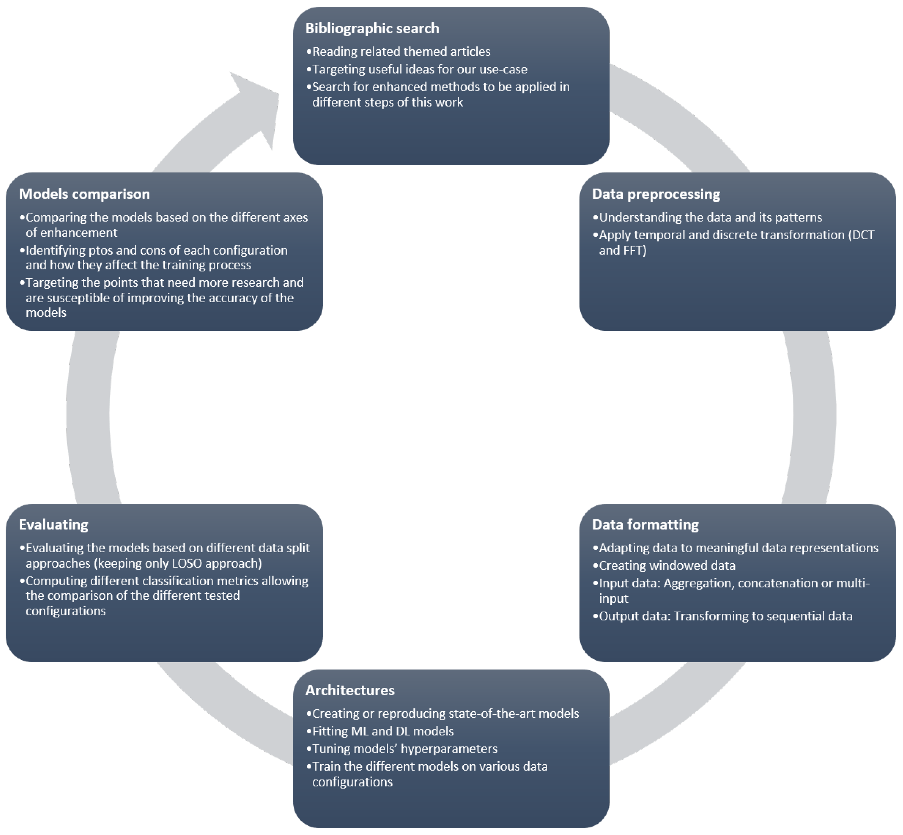
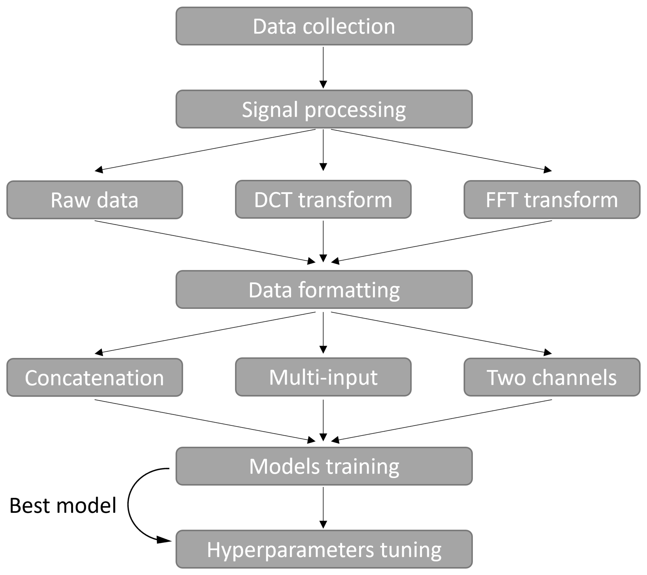
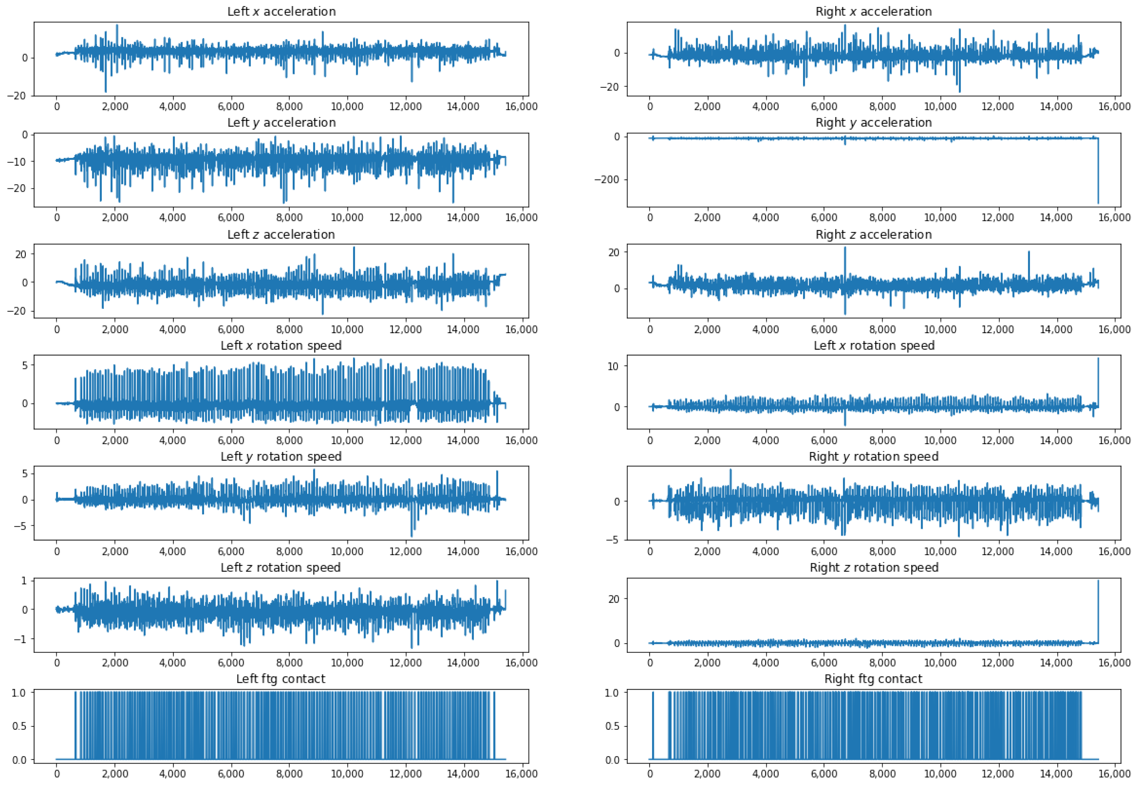
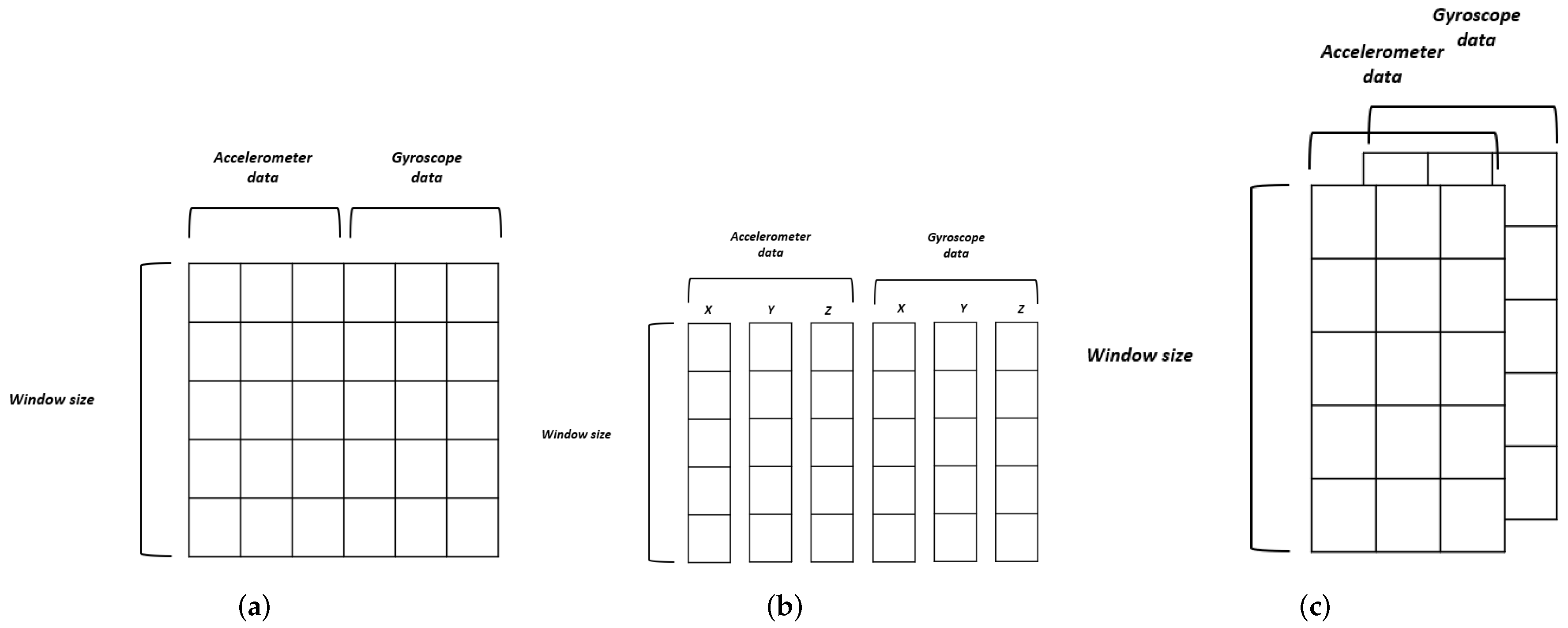
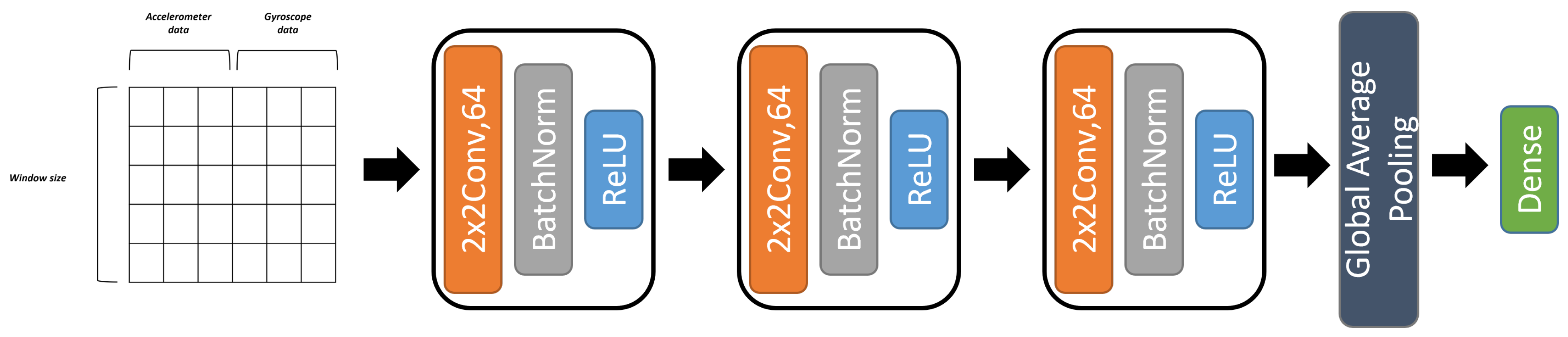
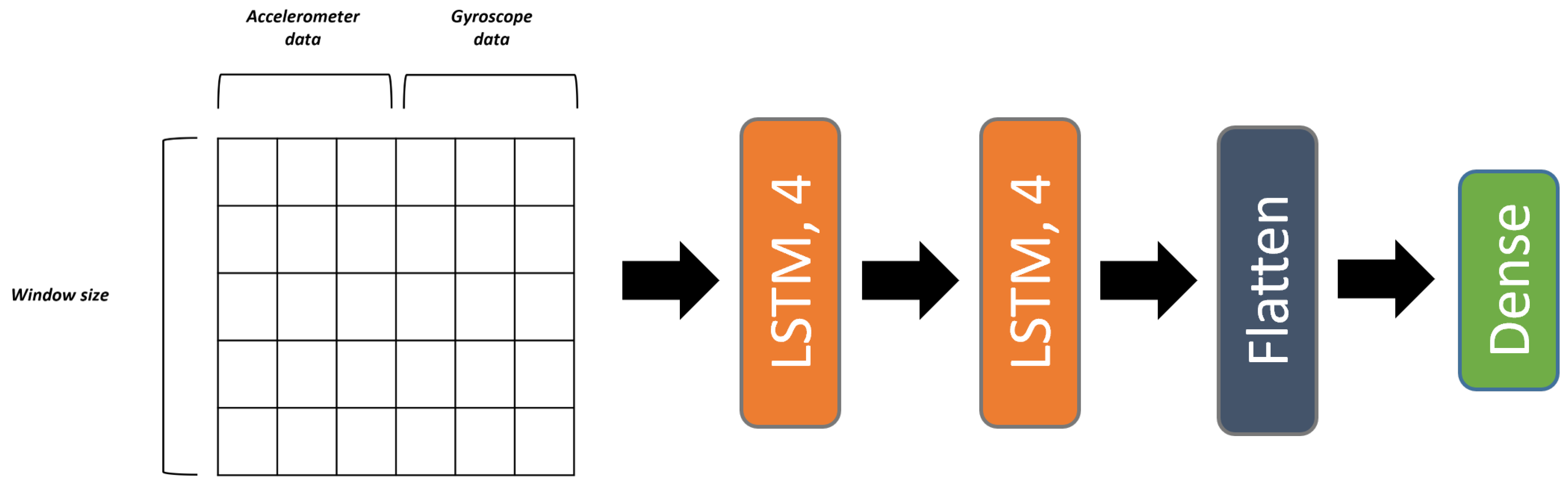
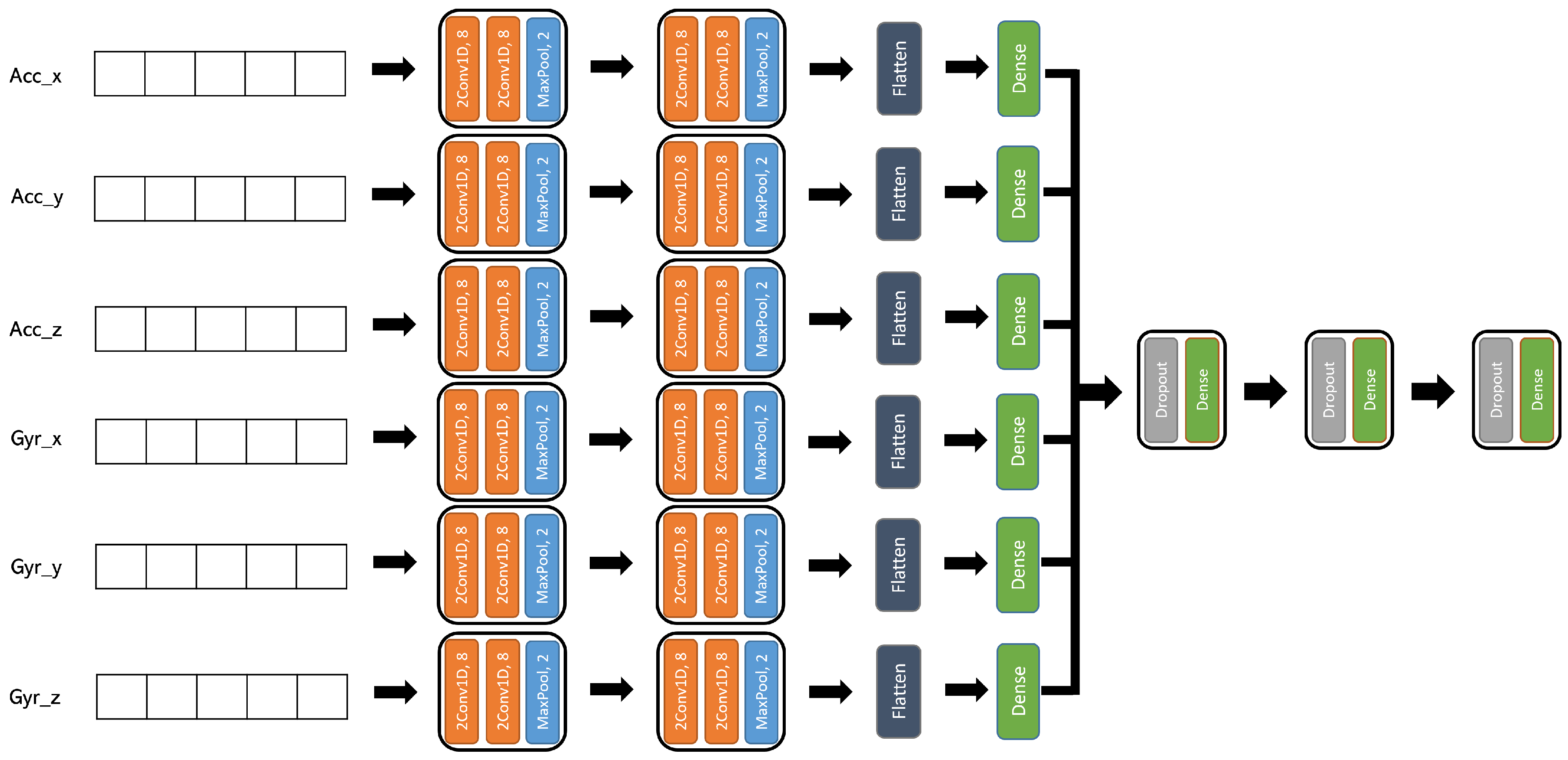
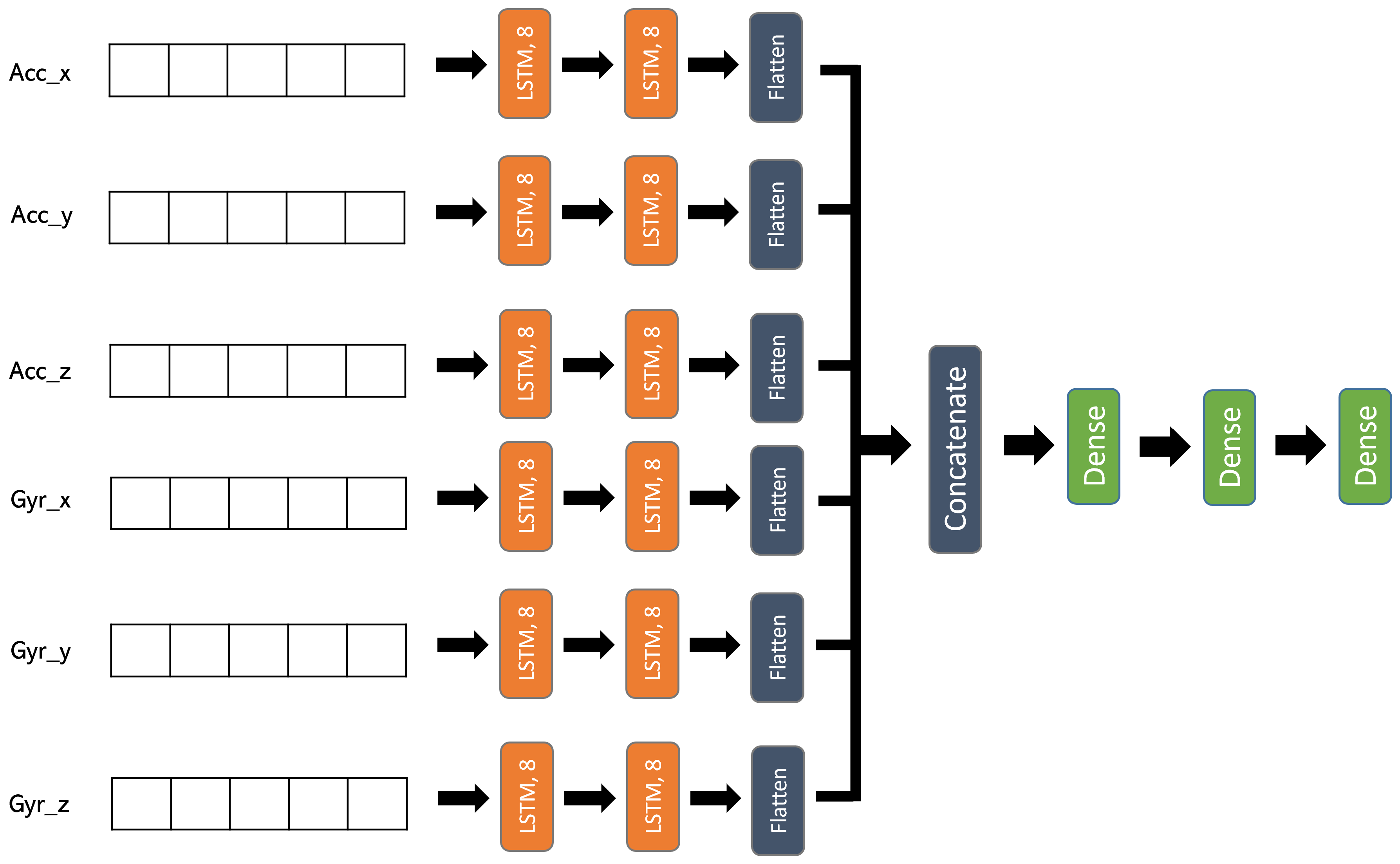
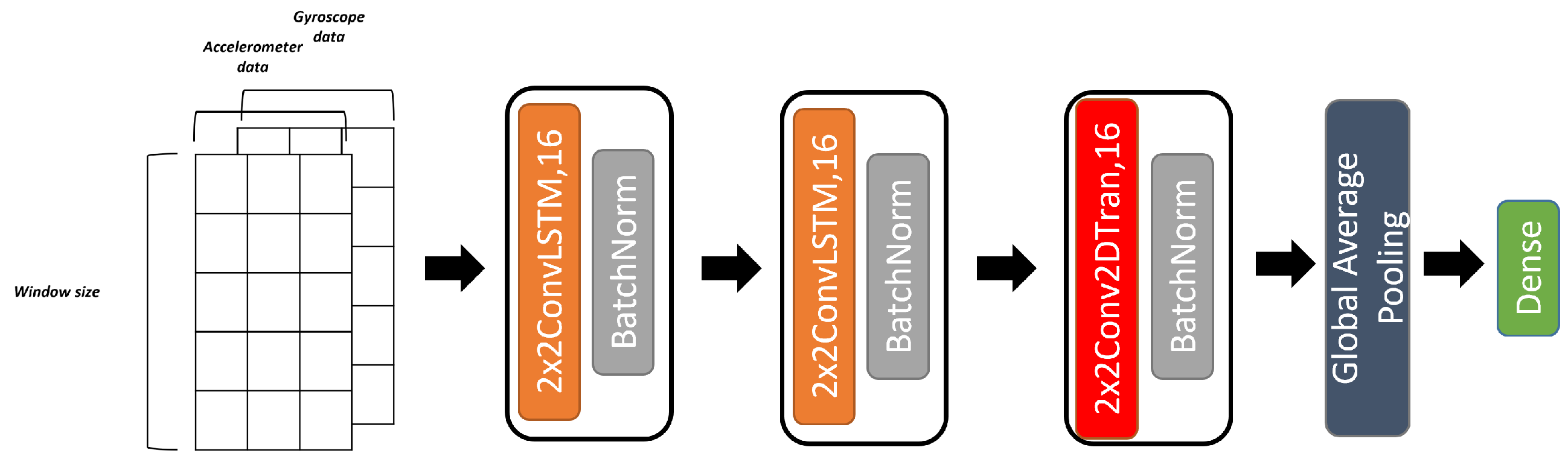
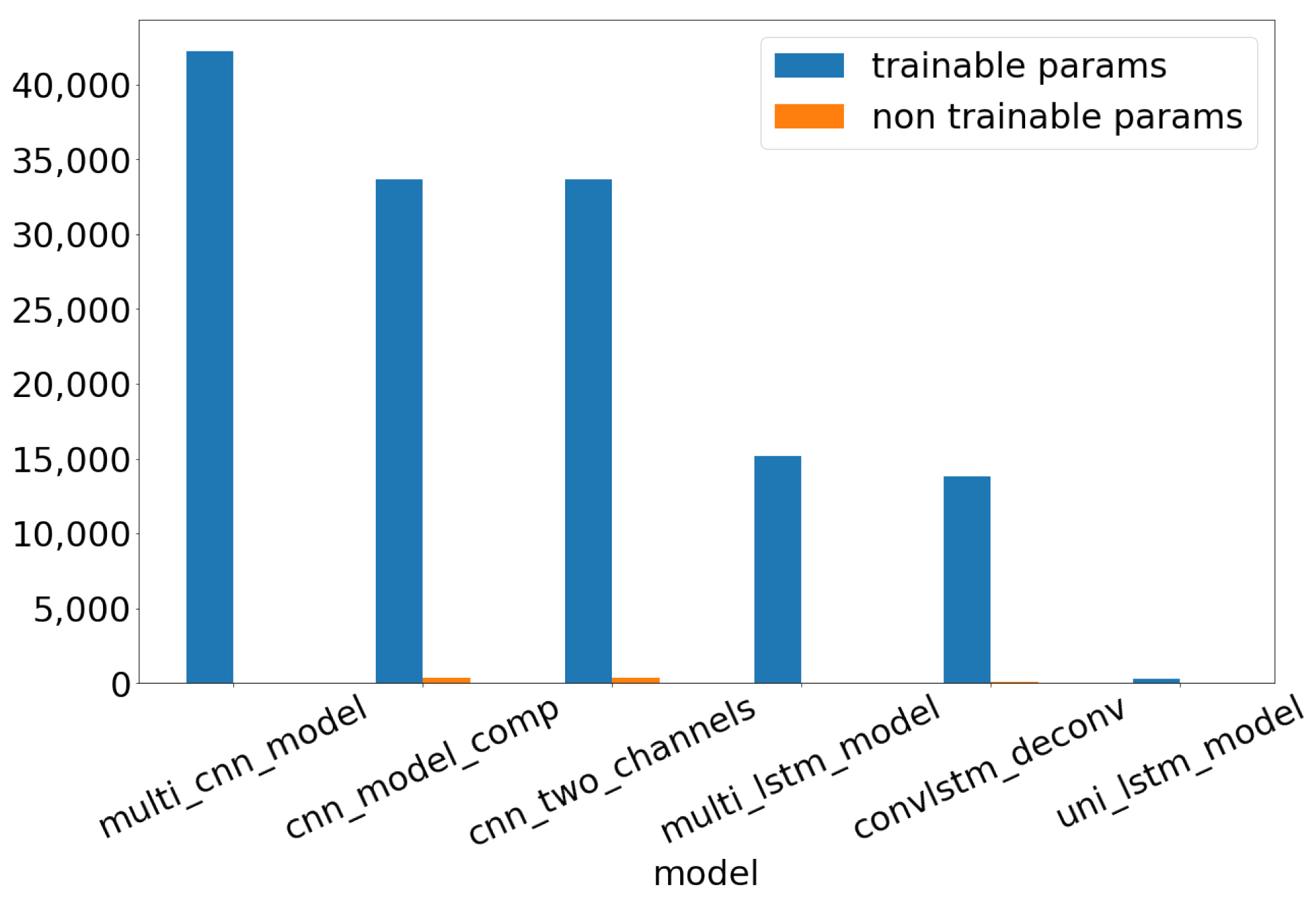
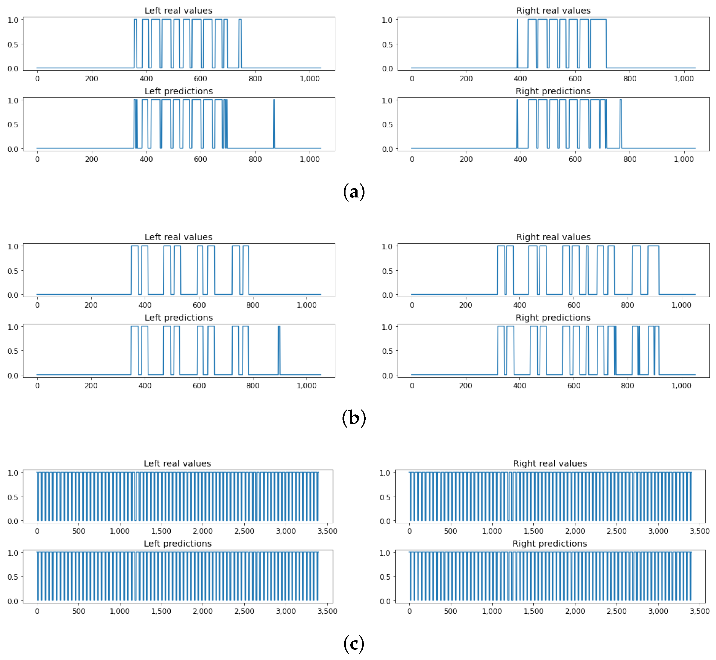
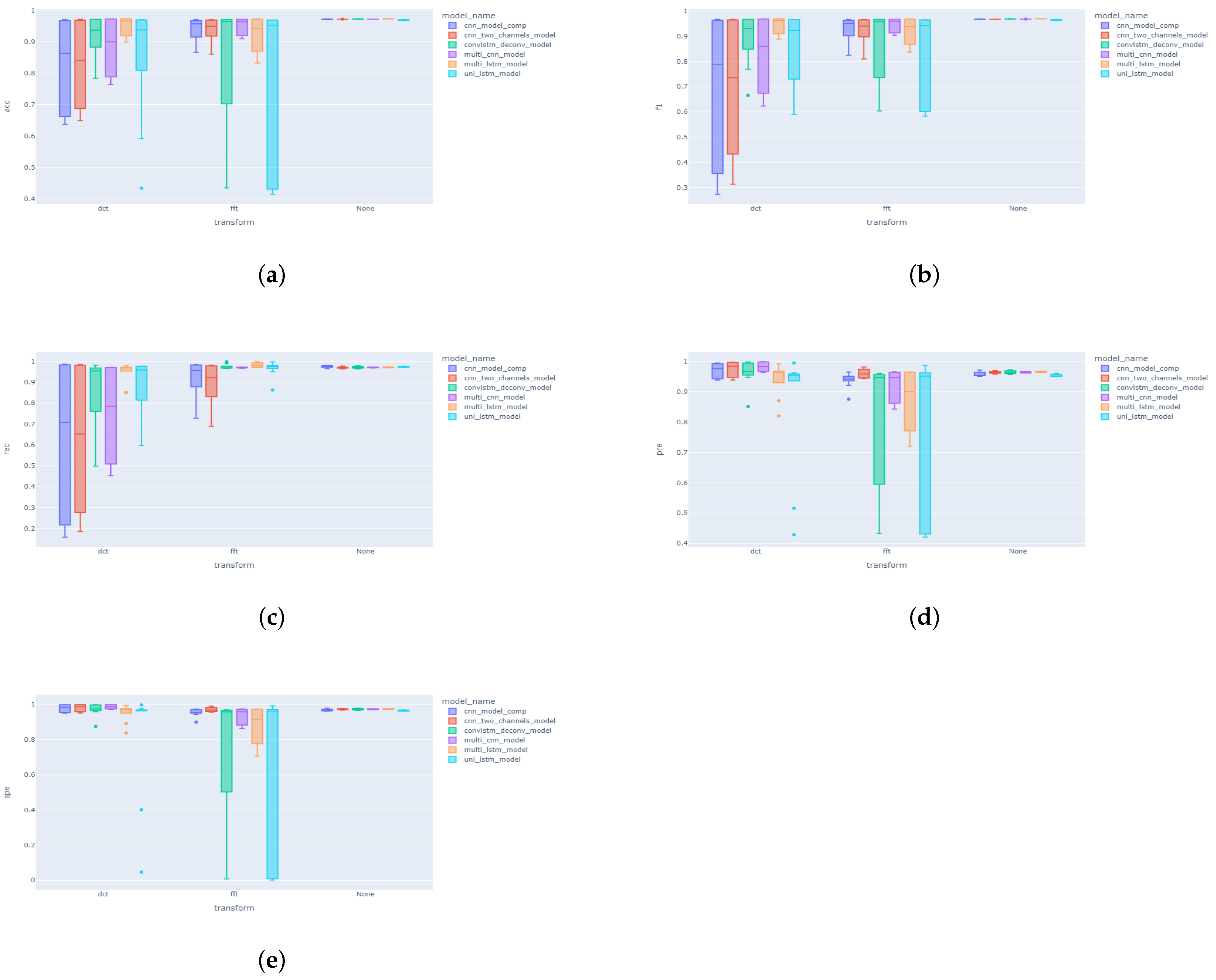