Article

Metaheuristic Extreme Learning Machine for Improving Performance of Electric Energy Demand Forecasting

by
Sarunyoo Boriratrit
1,2,
Chitchai Srithapon
3,
Pradit Fuangfoo
2 and
Rongrit Chatthaworn
1,*
1
Department of Electrical Engineering, Faculty of Engineering, Khon Kaen University, Khon Kaen 40002, Thailand
2
Provincial Electricity Authority of Thailand (PEA), Bangkok 10900, Thailand
3
Department of Electrical Engineering, KTH Royal Institute of Technology, 11428 Stockholm, Sweden
*
Author to whom correspondence should be addressed.
Submission received: 16 March 2022 / Revised: 21 April 2022 / Accepted: 24 April 2022 / Published: 27 April 2022
(This article belongs to the Special Issue Computing, Electrical and Industrial Systems 2022)

Abstract

:
Electric energy demand forecasting is very important for electric utilities to procure and supply electric energy for consumers sufficiently, safely, reliably, and continuously. Consequently, the processing time and accuracy of the forecast system are essential to consider when applying in real power system operations. Nowadays, the Extreme Learning Machine (ELM) is significant for forecasting as it provides an acceptable value of forecasting and consumes less computation time when compared with the state-of-the-art forecasting models. However, the result of electric energy demand forecasting from the ELM was unstable and its accuracy was increased by reducing overfitting of the ELM model. In this research, metaheuristic optimization combined with the ELM is proposed to increase accuracy and reduce the cause of overfitting of three forecasting models, composed of the Jellyfish Search Extreme Learning Machine (JS-ELM), the Harris Hawk Extreme Learning Machine (HH-ELM), and the Flower Pollination Extreme Learning Machine (FP-ELM). The actual electric energy demand datasets in Thailand were collected from 2018 to 2020 and used to test and compare the performance of the proposed and state-of-the-art forecasting models. The overall results show that the JS-ELM provides the best minimum root mean square error compared with the state-of-the-art forecasting models. Moreover, the JS-ELM consumes the appropriate processing time in this experiment.

Graphical Abstract

1. Introduction

For several decades, electric energy has been essential for living, and it is a basic utility that governments must provide for their people. Indeed, power utilities or electricity providers must procure and supply electric energy to consumers sufficiently, safely, reliably, and continuously [1]. In order to achieve all those factors previously mentioned, forecasting electric energy demand is necessary for utilities. Forecasting is the famous well-known method that learns the historical data and then predicts the expected data [2]. Many works have used various forecasting models [3], such as the dynamic regression model [4], ARIMA model [5], exponential smoothing model [6], neural network model [7], and so on, to generate the trend of future forecasted data and select the best model that is evaluated from its performance and accuracy.
Many researchers have proposed machine learning models to increase the accuracy of electric energy demand forecast. Gholamreza Memarzadeh and Farshid Keynia [8] proposed the new optimal long short-term memory model to predict electric energy demand and price based on Pennsylvania, New Jersey, and Maryland databases. Zongying Liu et al. [9] proposed the novel adaptive method applied with the kernel ELM model called the error-output recurrent two-layer ELM and used the quantum particle swarm optimization to increase the forecast accuracy of the time-series predicted demand. Mikel Larrea et al. [10] proposed the particle swarm optimization algorithm to optimize weight parameters in the ensemble ELM model for forecasting the Spanish time-series electric consumption. Yanhua Chen et al. [11] proposed the empirical mode decomposition to decompose the time-series forecasting data and mixed kernel with radial basis function and UKF to implement on the ELM model. The New South Wales, Victoria, and Queensland electric load databases were used for testing the proposed model. Qifang Chen et al. [12] proposed the novel deep learning model by using the stacked auto-encoder framework applied to the ELM model to improve the capabilities of forecasting. Moreover, the raw time-series data were analyzed by using the empirical mode decomposition method. Shafiul Hasan Rafi et al. [13] proposed the hybrid methodology of deep learning by integrating the convolutional neural network and long short-term memory to improve the forecast accuracy for forecasting the Bangladesh power system dataset. Muhammad Sajjad et al. [14] proposed the hybrid convolutional neural network and gated recurrent units to maximize forecast performance for appliance energy demand and individual household electric power demand. Yusha Hu et al. [15] proposed the optimization methods consisting of the genetic algorithm and particle swarm optimization applied to the backpropagation model to forecast the electric demand dataset. Mohammad-Rasool Kazemzadeh et al. [16] proposed the novel hybrid optimization method, which combines the particle swarm optimization with a machine learning model, to forecast the long-term electricity peak demand and electric energy demand. Ghulam Hafeez et al. [17] proposed the novel hybrid model of modified mutual information, factored condition restricted Boltzmann machine, and genetic wind driven optimization to forecast the hourly load data of FE, Dayton, and EKPC USA power grids.
From the aforementioned works, one of the machine learning models that can learn rapidly and provide acceptable results is the Extreme Learning Machine (ELM) [18]. The concept of this model is to learn the data without iterative tuning in the hidden layer phase and then calculate the output weight parameter with a pseudo-inverse matrix called the Moore–Penrose inverse matrix [19] in the output layer phase. However, the disadvantage of the ELM model [20,21,22] is that it uses the standard randomization of the input weight to compute in the input layer phase that can cause overfitting and has a high probability to fall into local optima.
To improve the performance of the electric energy demand forecasting model, this paper proposes a method to develop the ELM model by using metaheuristic optimization algorithms to adjust the appropriate result of the output weight, which can reduce the cause of overfitting. The Jellyfish Search Optimization (JSO) [23], the Harris Hawk Optimization (HHO) [24], and the Flower Pollination Algorithm (FPA) [
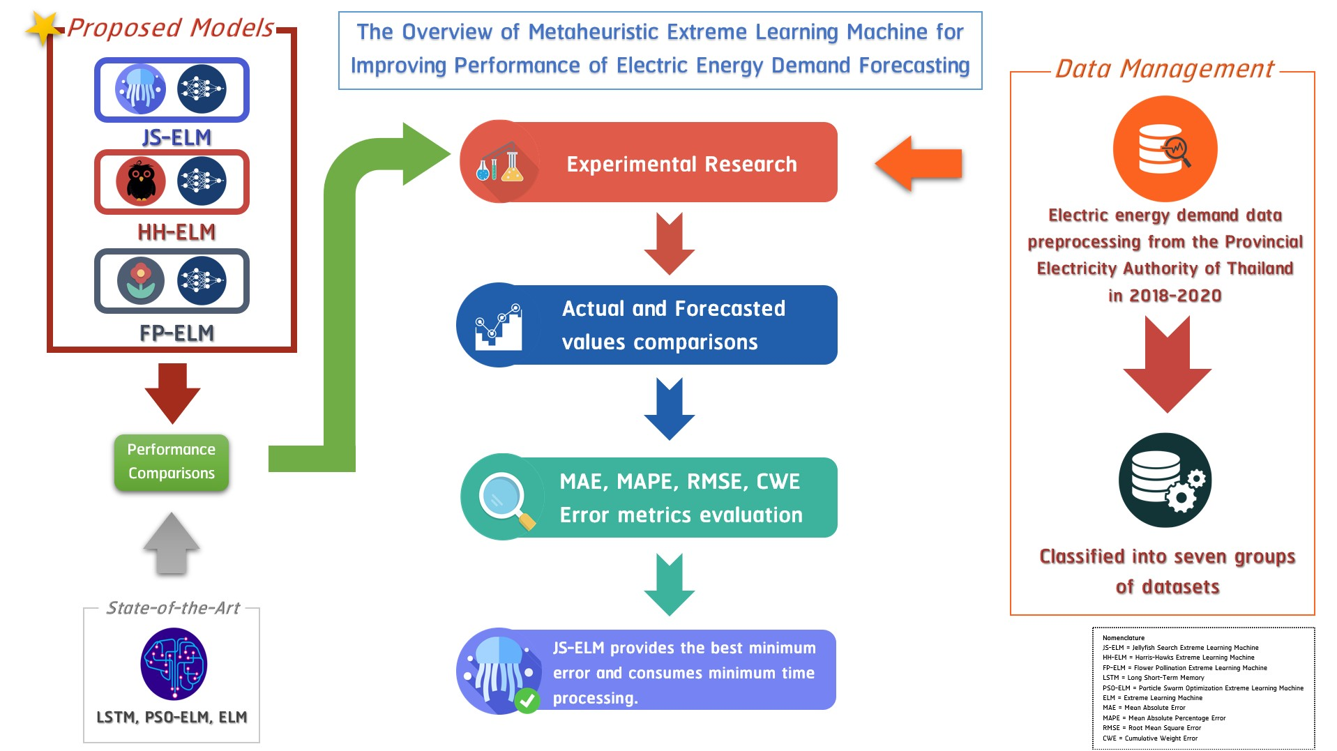
25] were selected for adjusting the output weight and reducing the cause of overfitting as mentioned before. The performances of these three proposed forecasting models were evaluated via an experiment that used the seven groups of the electric energy demand datasets in Thailand. The main contributions of this work can be summarized as follows:
  • This paper presents the novel hybrid method combining the ELM and metaheuristic optimization consisting of the JSO, the HHO, and the FPA to forecast the electric energy demand. Furthermore, the proposed model is investigated with the real-life dataset of electric energy demand to challenge the forecasting performance in terms of forecasting accuracy and stability.
  • To increase the robustness of forecasting in the training and testing processes of the traditional ELM model, the randomization process of the initial weight parameter in the ELM is developed to obtain the optimal weight parameter. The proposed metaheuristic optimization algorithms are not complex to implement, leading to less processing time, low population usage, and fast convergence to the optimal solution. In addition, these three optimization methods can reduce the number of hidden nodes of the ELM model.
  • Finally, the presented metaheuristic algorithms (the JSO, the HHO, and the FPA) have the characteristic of being self-adaptive to tune the weight parameter of the ELM without trapping in the local optima. This characteristic can increase the forecasting stability of the traditional model. Furthermore, this method can reduce the cause of sensitivity to outliers, which leads the forecasting process to be more stable, and the standard deviation was used to calculate the forecasting stability of the proposed models.
This paper is organized as follows. Section 2 indicates the basic principles of the algorithms used in this paper. Section 3 indicates the methodology of the datasets’ preparation and the proposed models. Section 4 indicates the overall experimental results using the datasets and the proposed models in Section 3. Lastly, the conclusion and future work of this work are described in Section 5.

2. Basic Principles

This section describes the basic principles and materials used in this research, which consists of forecasting methodology, ELM, JSO, HHO, FPA, a summary of selected metaheuristic optimization, and related works as shown below.

2.1. Forecasting Methodology

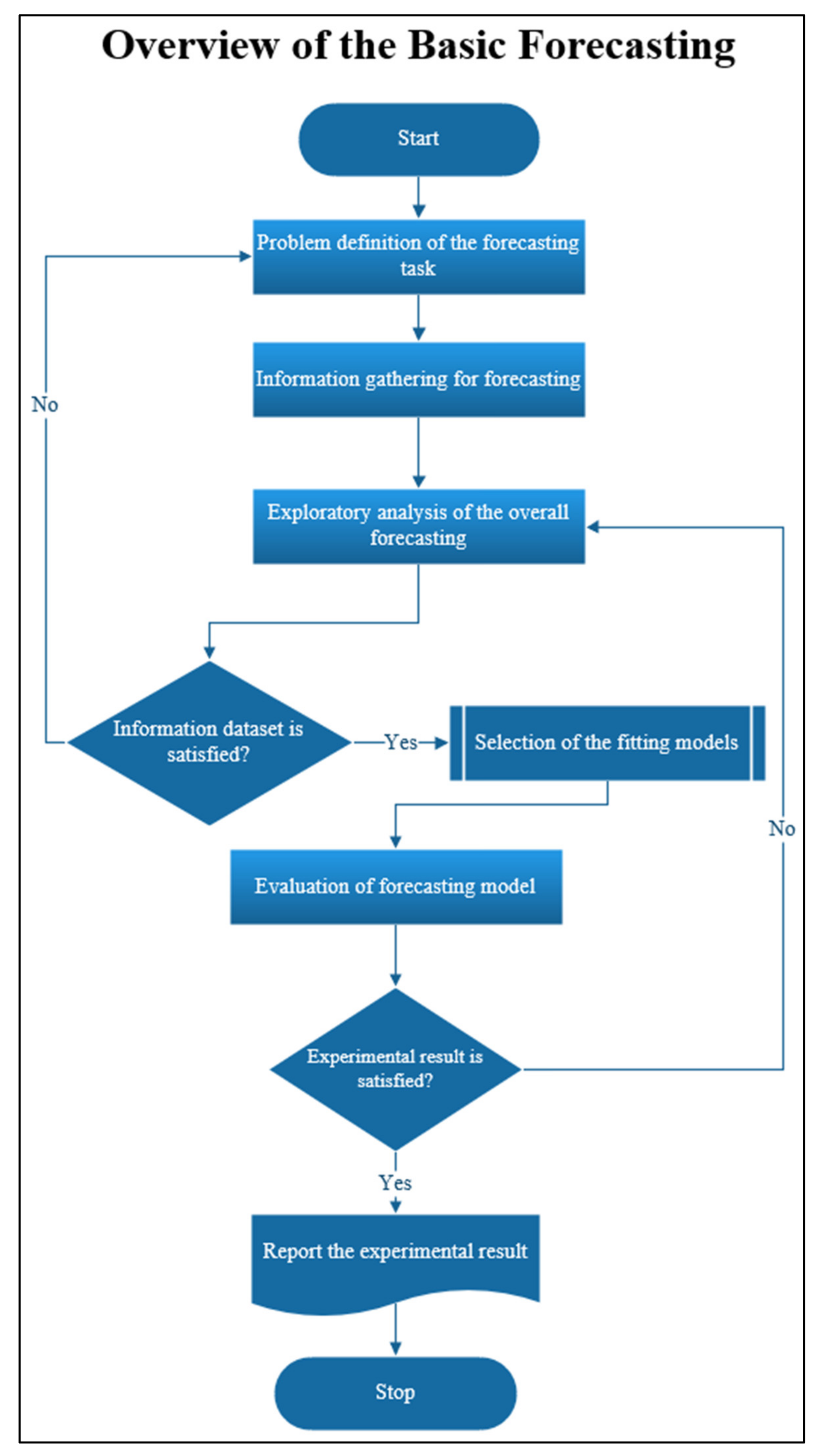
The basic methodology for forecasting (Figure 1) can be described in five steps [26] as follows. Firstly, the forecasting task problem is defined; the aim of this step is to study the problem and factors that can affect the outcome of forecasting. Secondly, the information is gathered for forecasting; the aim of this step is to collect and analyze the significant data needed for forecasting and finding the expected result [27]. Thirdly, the exploratory analysis of the overall forecasting is conducted; the aim of this step is to actively analyze the consistency of data to so that they can be implement without noise or elements missing in the dataset such as the imbalance or inconsistency of data [28], missing values of data [29], and so on. Fourthly, the fitting models are selected; this step is the key of this research, which proposes the new model to increase the performance of the forecasting. Fifthly, the evaluation of the forecasting model is conducted, this step aims to consider and evaluate the experimental results obtained from all models and then select the best model for forecasting. The performances of all models [30] can be compared by considering error metrics such as the Mean Absolute Error (MAE), Mean Absolute Percentage Error (MAPE), Root Mean Square Error (RMSE), and so on.

2.2. Extreme Learning Machine

The Extreme Learning Machine (ELM) was proposed by Guang-Bin Huang et al. [18]. Due to the non-iterative tuning model, the training time of the ELM model was faster than other machine learning models in the hidden layer.
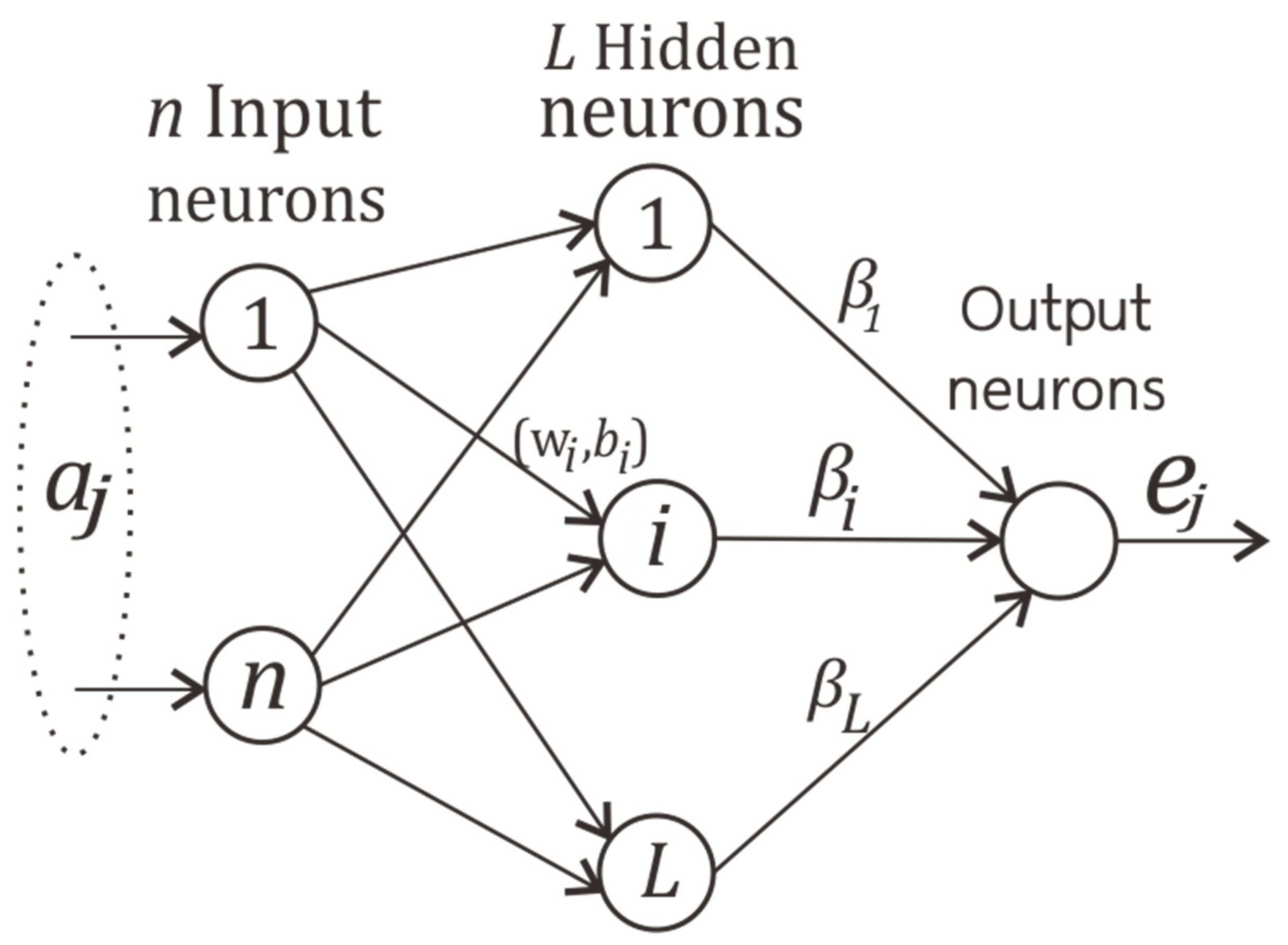
Figure 2 is the architecture of the ELM model. The structure of this model has three layers. The first layer is the input layer, which imports the sample dataset a j , t j of input data a j = a j 1 , a j 2 , a j 3 , , a j n T R n and target data t j = t j 1 , t j 2 , t j 3 , , t j m T R m where n is the number of instances of data with j = 1 , 2 , , n . After the input layer step is completed, the second hidden layer is calculated as shown as in (1).
i = 1 L β i g i a j = i = 1 L β i g w i · a j + b i = e j
where w i is the initial weight randomization, β i is the connecting weight of hidden nodes and output nodes, L is the random number of hidden nodes, and g a is the activation function. Equation (1) can be revised to a short equation defined as the matrix, as in (2).
H β = T
where H = h a 1 h a N = G w 1 , b 1 , a 1 G w L , b L , a 1 G w 1 , b 1 , a N G w L , b L , a N N   x   L   β = β 1 T β L T L   x   m and T = t 1 T t L T N   x   m .
After the hidden layer step is completed, the aim of the third output layer step is to find the β matrix; Equation (2) is inversed to Equation (3) as shown below.
β = H T
where H is the Moore–Penrose pseudo-inverse [19] of the H matrix.
Due to the problem of overfitting of the ELM model [20], this paper proposes a method to find the optimal weight parameter with the metaheuristic optimization that can reduce the cause of the overfitting.

2.3. Jellyfish Search Optimization

Jellyfish Search Optimization (JSO) was proposed by Jui-Sheng Chou and Dinh-Nhat Truong [23]. The main idea of this optimization was inspired by the nature of jellyfish behavior in the ocean when hunting prey for their food [32]. 
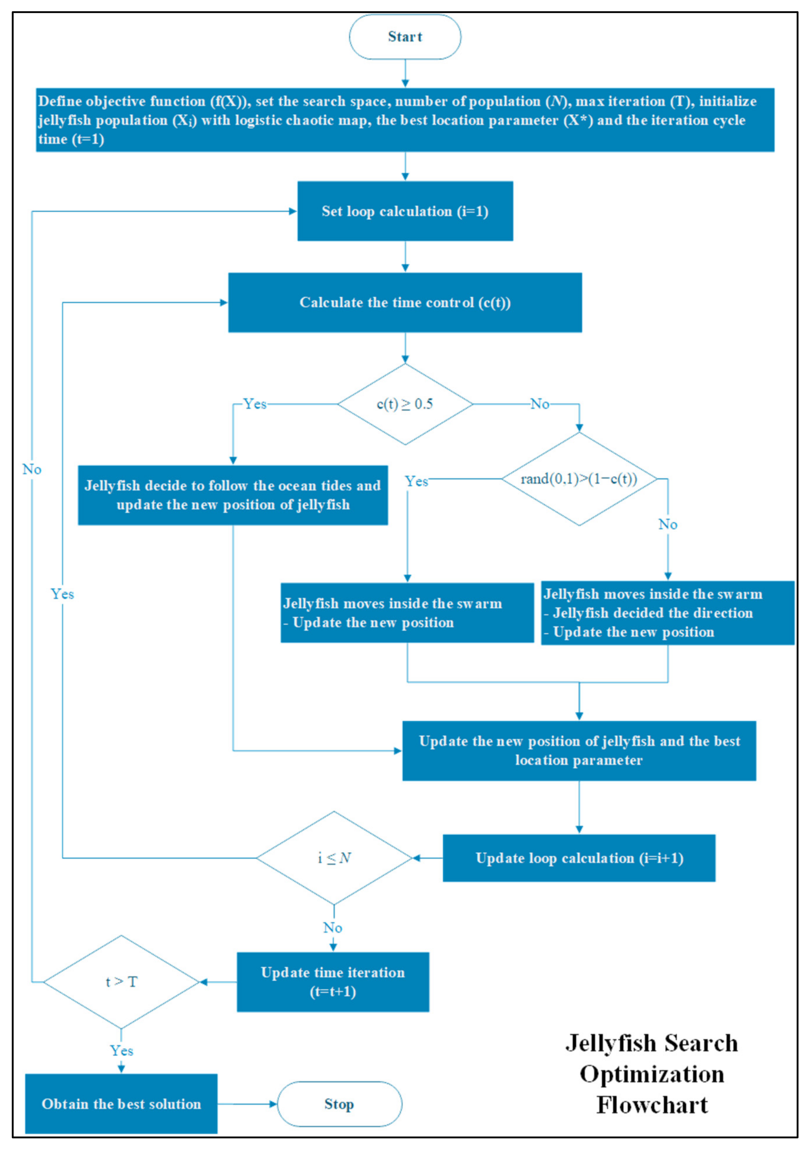
Figure 3 is the JSO algorithm flowchart that can be described as follows:
  • Define the objective function ( f X ) in terms of X = x 1 , , x d T , the best location parameter ( X ), the number of search space, the number of population ( N ), the max iteration ( T ), the iteration cycle time starting from 1 to max iteration ( t ). Jellyfish population X i is initialized with a logistic chaotic map [33].
  • Calculate the control time ( c t ) as presented in (4).
    c t = 1 1 T × 2 × r a n d 0 , 1 1
    where r a n d 0 , 1 is the number of randomization from 0 to 1, which changes in every iteration.
If the control time is greater than or equal to 0.5 ( c t 0.5 ), then the jellyfish decides to follow the ocean tides as shown in (5). Otherwise, the movement of jellyfish to the swarm is calculated by Equation (7).
t r e n d = X β × r a n d 0 , 1 × μ
where t r e n d is the direction of the ocean tides, β is a distribution coefficient that is greater than 0 ( β > 0 ) , and μ is the mean location of all jellyfishes.
After that, jellyfish live at the new position that can be calculated as shown as in (6).
X i t + 1 = X i t + r a n d 0 , 1 × X β × r a n d 0 , 1 × μ
If r a n d 0 , 1 is greater than 1 c t , then jellyfish show the passive motions, which can be calculated by Equation (7). Otherwise, jellyfish show the active motions by deciding the direction as shown by Equation (8).
X i t + 1 = X i t + γ × r a n d 0 , 1 × U b L b
where γ is the motion coefficients, and U b and L b are upper bound and lower bound, respectively.
S t e p = X i t + 1 X i t = r a n d 0 , 1 × D i r e c t i o n
where S t e p is the direction of the movement of jellyfish and D i r e c t i o n can be decided by Equation (9).
D i r e c t i o n = X j t X i t X i t X j t       i f   f X i f X j     i f   f X i < f X j
3.
Update the new position of the jellyfish and the best location parameter.
4.
Repeat step 2 until the iteration reaches the max iteration criterion.
The JSO algorithm is used to optimize the weight parameter in the ELM model that is described in Section 3.3.

2.4. Harris Hawk Optimization

The Harris Hawk Optimization (HHO) was proposed by Ali Asghar Heidari et al. [24]. The main idea of this optimization model came from the cooperative behavior and hunting of prey of Harris Hawk [34]. 
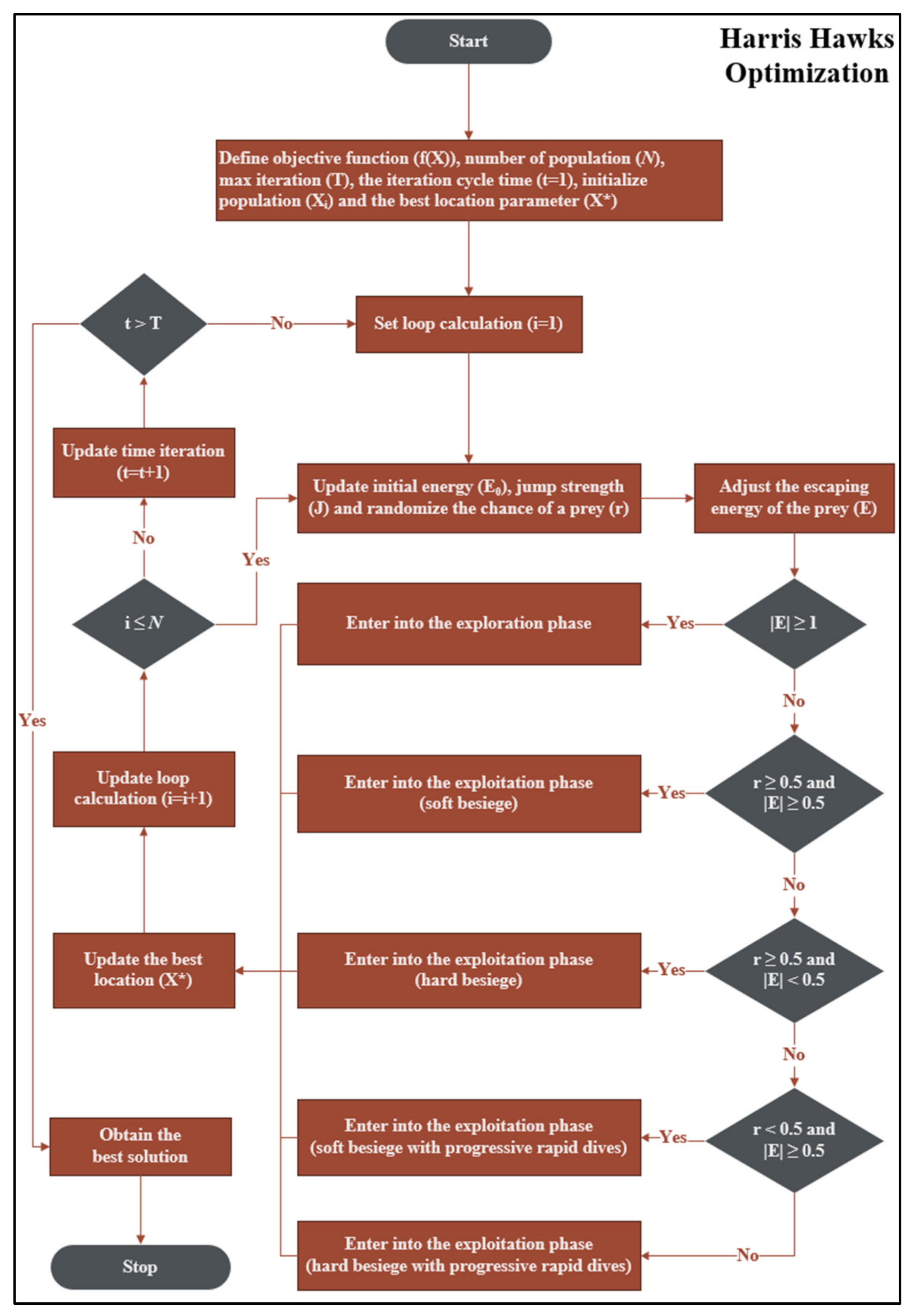
Figure 4 presents a flowchart of the HHO algorithm that can be described as follows:
  • Define the objective function ( f X ) in terms of X = x 1 , , x d T , the location of rabbit (best location parameter) ( X ), the number of population ( N ), the max iteration ( T ), the iteration cycle time starting from 1 to max iteration ( t ), and initialize hawk population X i .
  • Specify the initial energy E 0 as in (10).
    E 0 = 2 × r a n d 0 , 1 1
  • Specify the initial jump strength ( J ) as in (11).
    J = 2 × 1 r a n d 0 , 1
  • Adjust the escaping energy of the prey ( E ) as in (12).
    E = 2 E 0 1 t T
  • If E 1 , then go to the exploration phase as in (13).
    If   q 0.5 :     X t + 1 = X r a n d t r a n d 1 0 , 1   X r a n d t 2 r a n d 2 0 , 1 X t If   q < 0.5 :   X t + 1 = X X m t r a n d 3 0 , 1 L b + r a n d 4 0 , 1 U b L b
    where X r a n d t is the random position of the currently selected hawk, X m t is the average position of the current population, and q is random numbers between 0 and 1.
  • If E < 1 , then consider with four conditions of the exploitation phase as follows:
    6.1.
    If the instantly randomized number r is greater than or equal to 0.5 r 0.5 and E 0.5 , then go to the soft besiege as in (14).
    X t + 1 = X X t E J X X t
    6.2.
    If r 0.5 and E < 0.5 , then go to the hard besiege as in (15).
    X t + 1 = X E X X t
    6.3.
    If r < 0.5 and E 0.5 , then go to the soft besiege with progressive rapid dives as in (16).
    X t + 1 = Y i f   f Y < f X t Z i f   f Z < f X t
    where Y is the next movement of the hawk as in (17).
    Y = X E J X X t
    and Z is the random movement of the hawk with the levy flight concept as in (18).
    Z = X E J X X t   S × L F D
    where D is the dimension of the problem, S is the 1 × D size of random vector and L F is the levy flight function [35] as in (19).
    L F = 0.01 × r a n d 0 , 1 × Γ 1 + β × s i n π β 2 Γ 1 + β 2 × β × 2 β 1 2 1 β r a n d 0 , 1 1 β
    where β is the default constant set to 1.5.
    6.4.
    If r < 0.5 and E < 0.5 , then go to the hard besiege with progressive rapid dives as in (20).
    X t + 1 = Y i f   f Y < f X t Z i f   f Z < f X t
    where Y is the next movement of the hawk as in (21).
    Y = X E J X X m t
    and Z is the random movement of the hawk with levy flight concept as in (22).
    Z = X E J X X m t S × L F D
  • Update the new position of the hawk and the location of the rabbit (best location parameter).
  • Repeat step 4 until the iteration reaches the max iteration criterion.
The HHO algorithm is used to optimize the weight parameter in the ELM model that is described in Section 3.3.

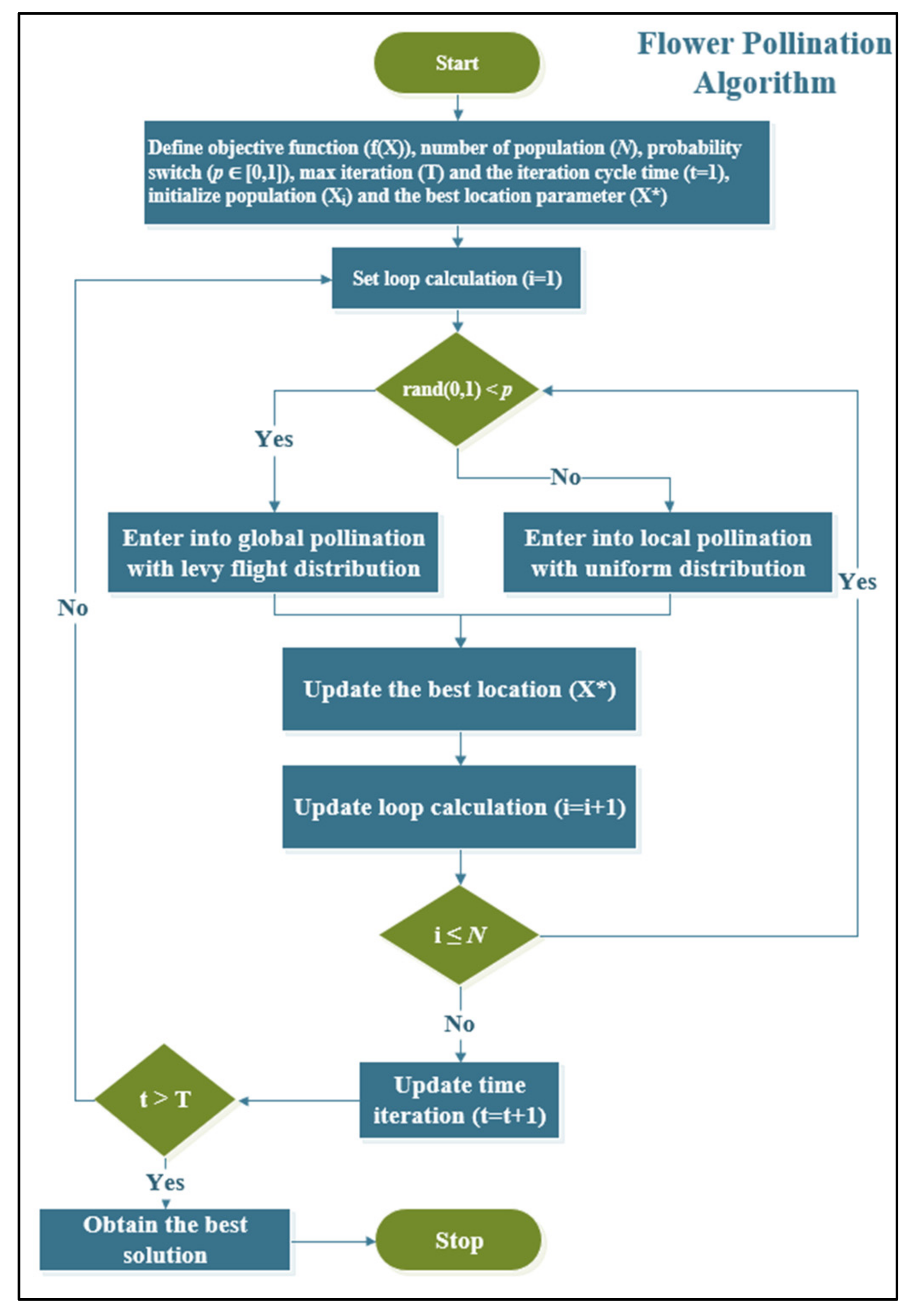
2.5. Flower Pollination Algorithm

The Flower Pollination Algorithm (FPA) was proposed by Xin-She Yang [25]. The main idea of this optimization model was inspired by the nature of the pollination process of flowers. Figure 5 presents the FPA algorithm flowchart that can be described as follows:
  • Define the objective function ( f X ) in terms of X = x 1 , , x d T , define the best location parameter ( X ), set the number of population ( N ), set the max iteration ( T ), set the iteration cycle time starting from 1 to max iteration ( t ), and initialize flower population X i and fixed switch probability set to 0.8 p = 0.8 .
  • Define the random number between 0 and 1 and compare it with switch probability. If r a n d 0 , 1 < p , then go to the global pollination phase as in (23). Otherwise, go to the local pollination phase as in (24).
    X i t + 1 = X i t + L F X i t X
    where LF is the levy flight function [35], which is defined as in (19).
    X i t + 1 = X i t + r a n d 0 , 1 × X j t X k t
    where X j t and X k t are other populations obtained from a random position in terms of t .
  • Update the new position of flowers and the best location parameter.
  • Repeat step 2 until the iteration reaches the max iteration criterion.
The FPA algorithm is used to optimize the weight parameter in the ELM model that is described in Section 3.3.

2.6. Summary of the JSO, the HHO, and the FPA

As aforementioned, the Jellyfish Search Optimization, the Harris Hawk Optimization, and the Flower Pollination Algorithm are the metaheuristic algorithms inspired by animals’ and plants’ behavior in nature [36,37]. According to Table 1, the benefits and drawbacks of the three metaheuristics are summarized. The benefits of JSO [23] include its fast speed to converge calculation, stability in the processing of the problem, and being hard to trap in local optima. However, the drawback of JSO is that there are quite a minor of related works because this optimization was a novel metaheuristics model in 2020. The benefit of HHO [38] is there are many steps of calculation that are hard to trap in local optima; however, the drawback of HHO is that it is slow to converge calculation. Finally, the benefits of FPA [39] are it is fast to converge calculation because the steps of this optimization are simple and easy to implement; however, the drawback of FPA is that it is easy to trap in local optima.
In conclusion, the three metaheuristic optimizations were merged with the ELM model to optimize the weight parameter, compare the three proposed models with the forecasting dataset, and evaluate the model with the error metrics objective function.

3. Data Preparation and Proposed Models

This section describes the technique of this research work, which consists of an overview of the electric energy demand datasets in Thailand, proposed data, and models used in the experiment to achieve the best result, the experimental setup and hyper-parameter settings for all proposed and state-of-the-art models, and performance evaluation of each model.

3.1. Preparation of Electric Energy Demand Data

Electric energy demand datasets were collected from Provincial Electricity Authority in Thailand (PEA), which can be accessed from references [40,41]. The scope of the electric energy demand datasets in this research was set from 2018 to 2020.
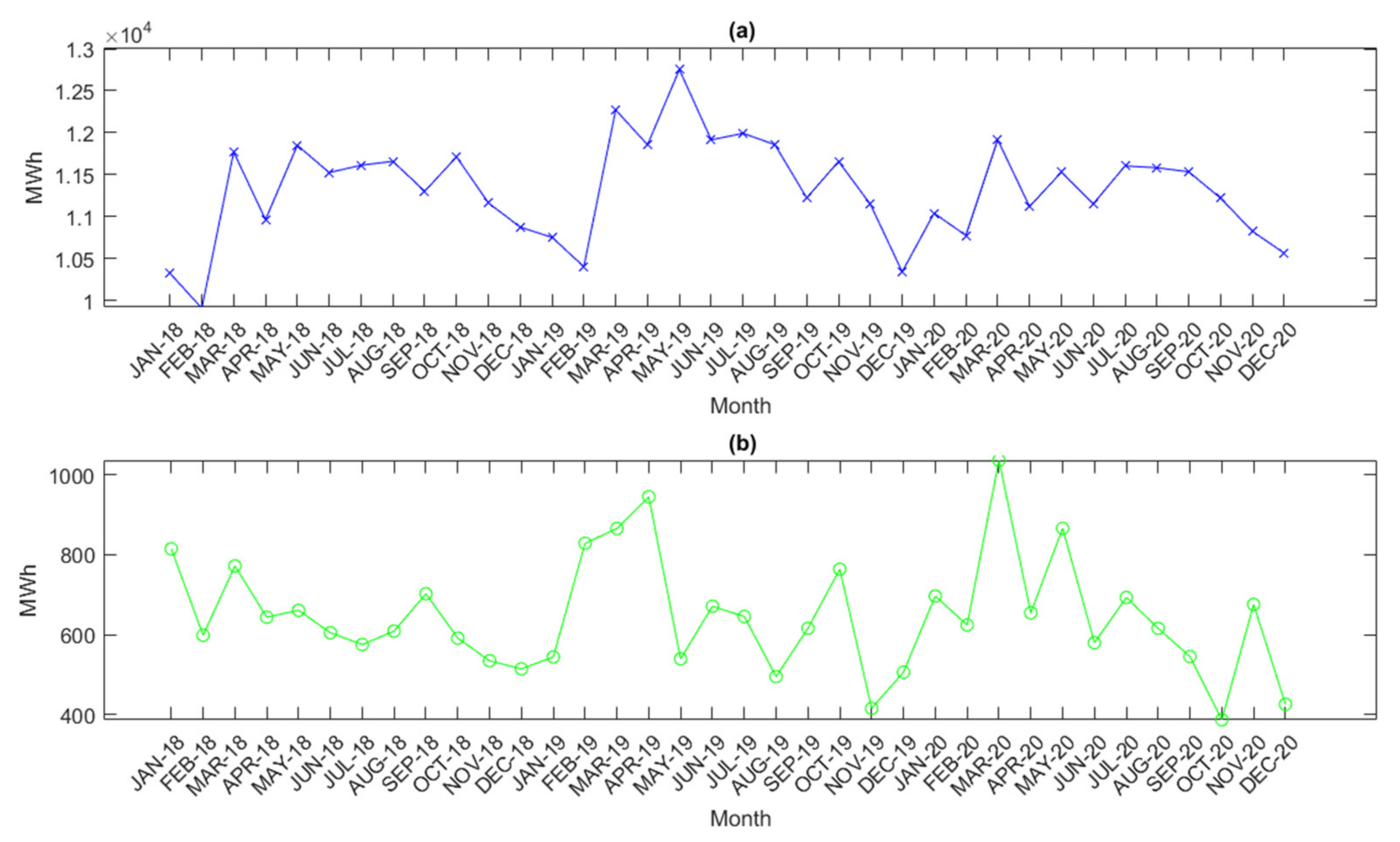
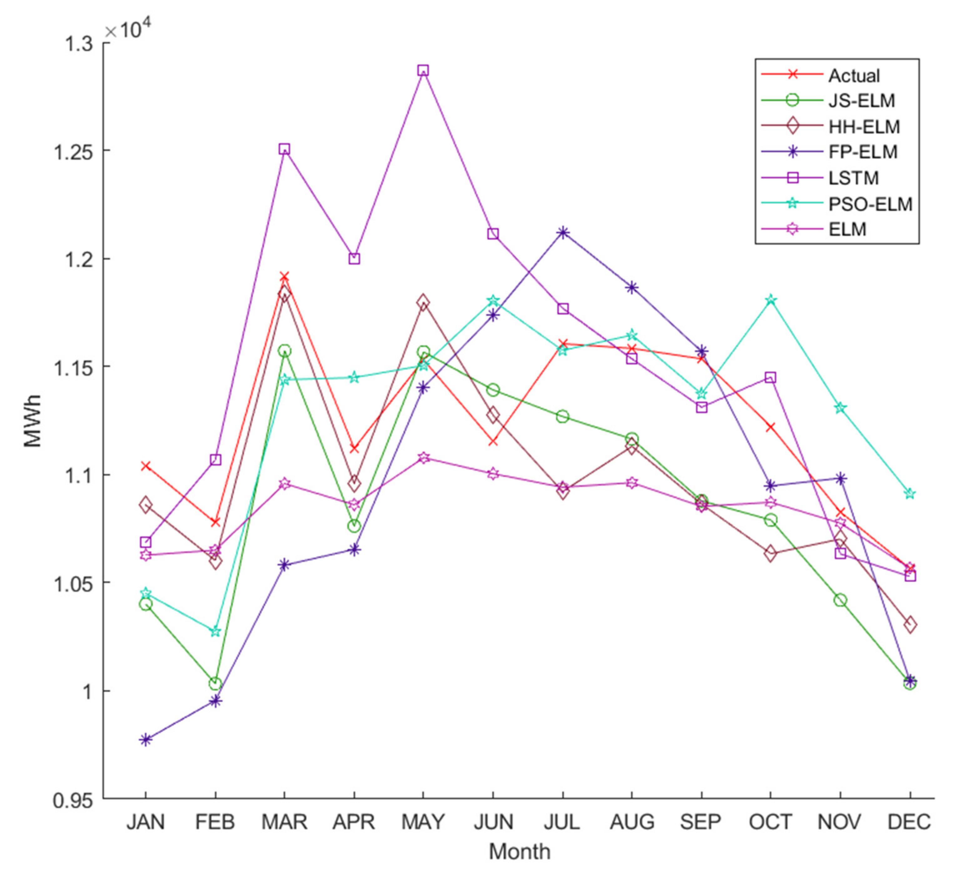
Figure 6a is the pattern of the monthly demand data of electric energy from January 2018 to December 2020 in terms of MegaWatt-Hour (MWh). The minimum electric energy demand is 9909 MWh in February 2018, the maximum electric energy is 12,752 MWh in May 2019, and the average electric energy demands in 2018, 2019, and 2020 are 11,222 MWh, 11,514 MWh, and 11,239 MWh, respectively. 
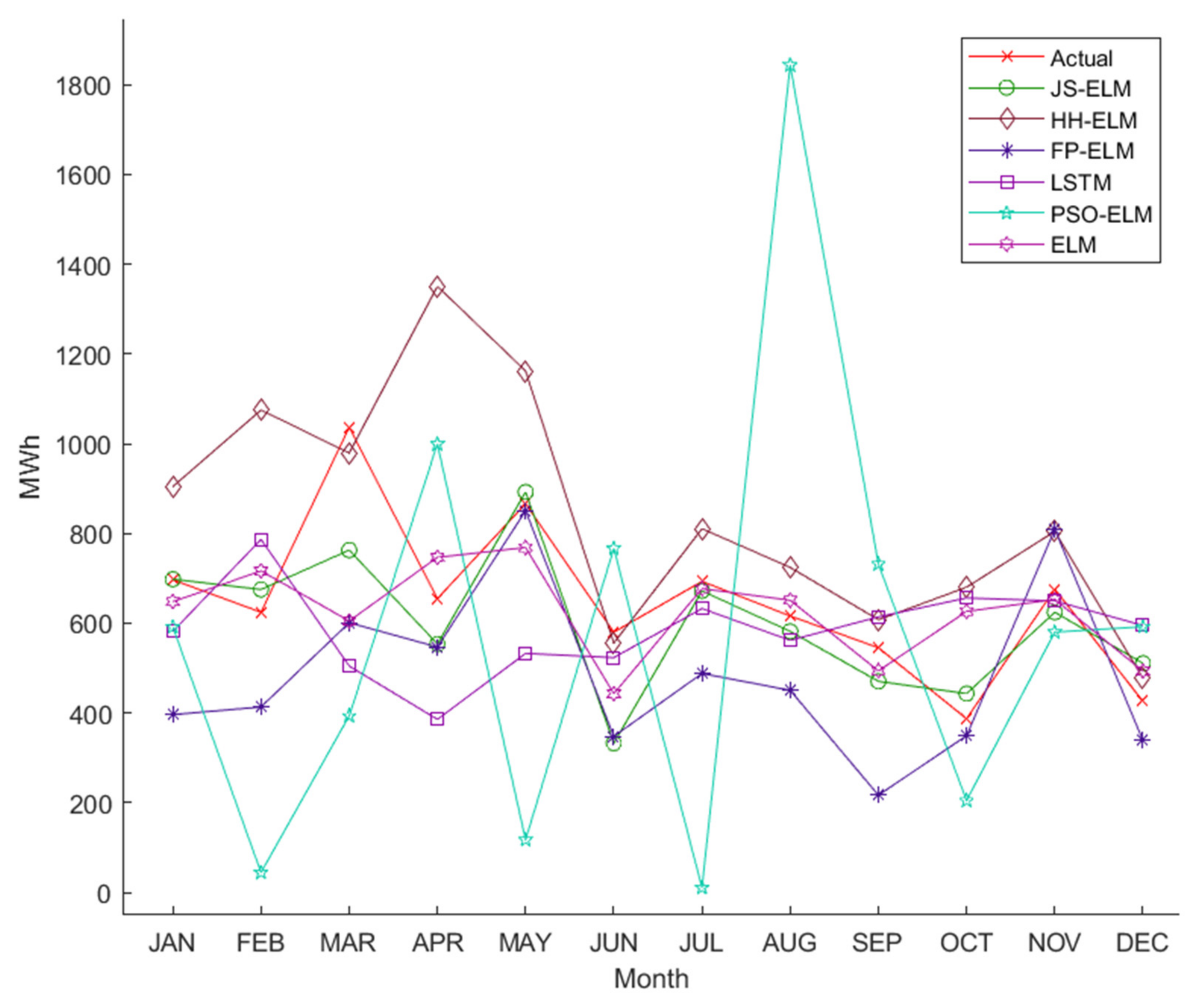
Figure 6b is the pattern of the monthly loss data of electric energy in Thailand from January 2018 to December 2020. The minimum loss is 387 MWh in October 2020, the maximum loss is 1036 MWh in March 2020, and the average losses in 2018, 2019, and 2020 are 635 MWh, 653 MWh, and 650 MWh, respectively.
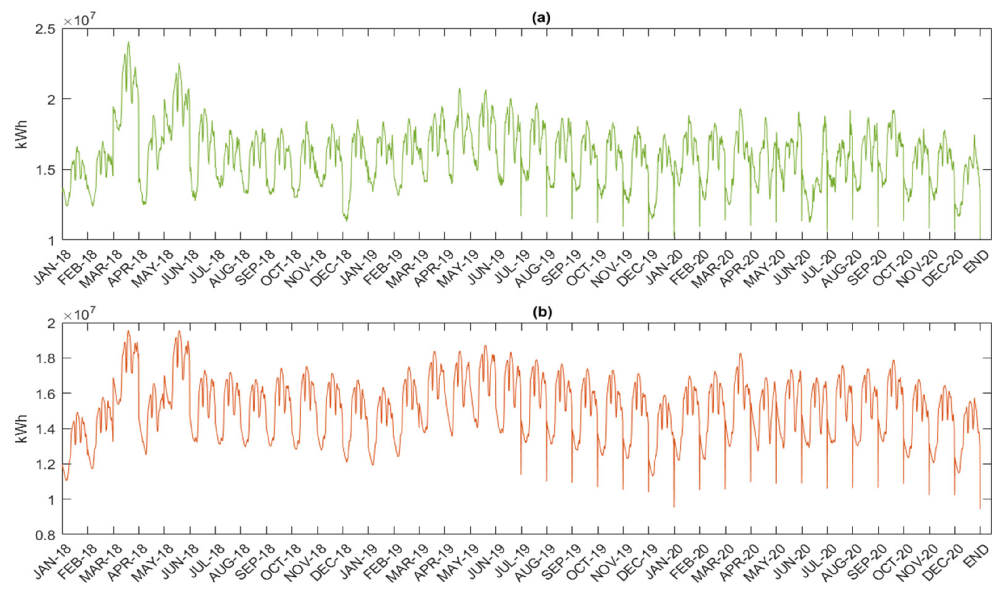
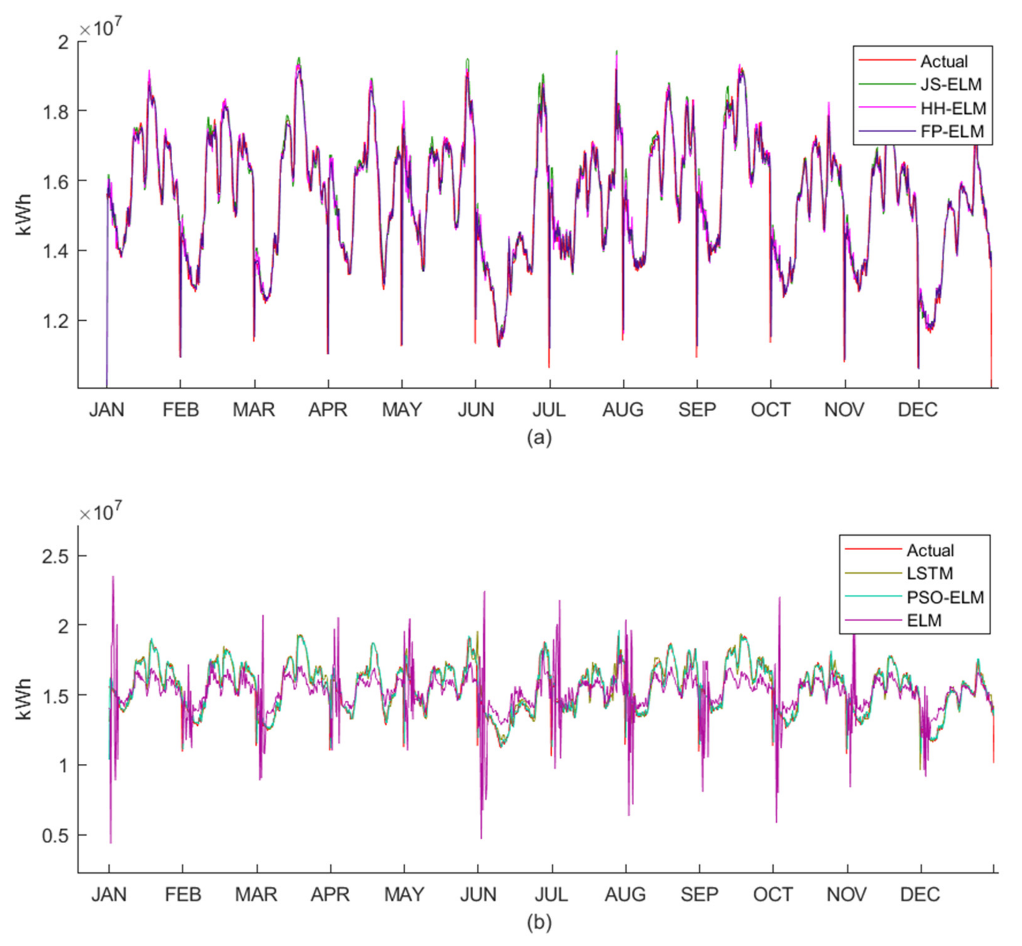
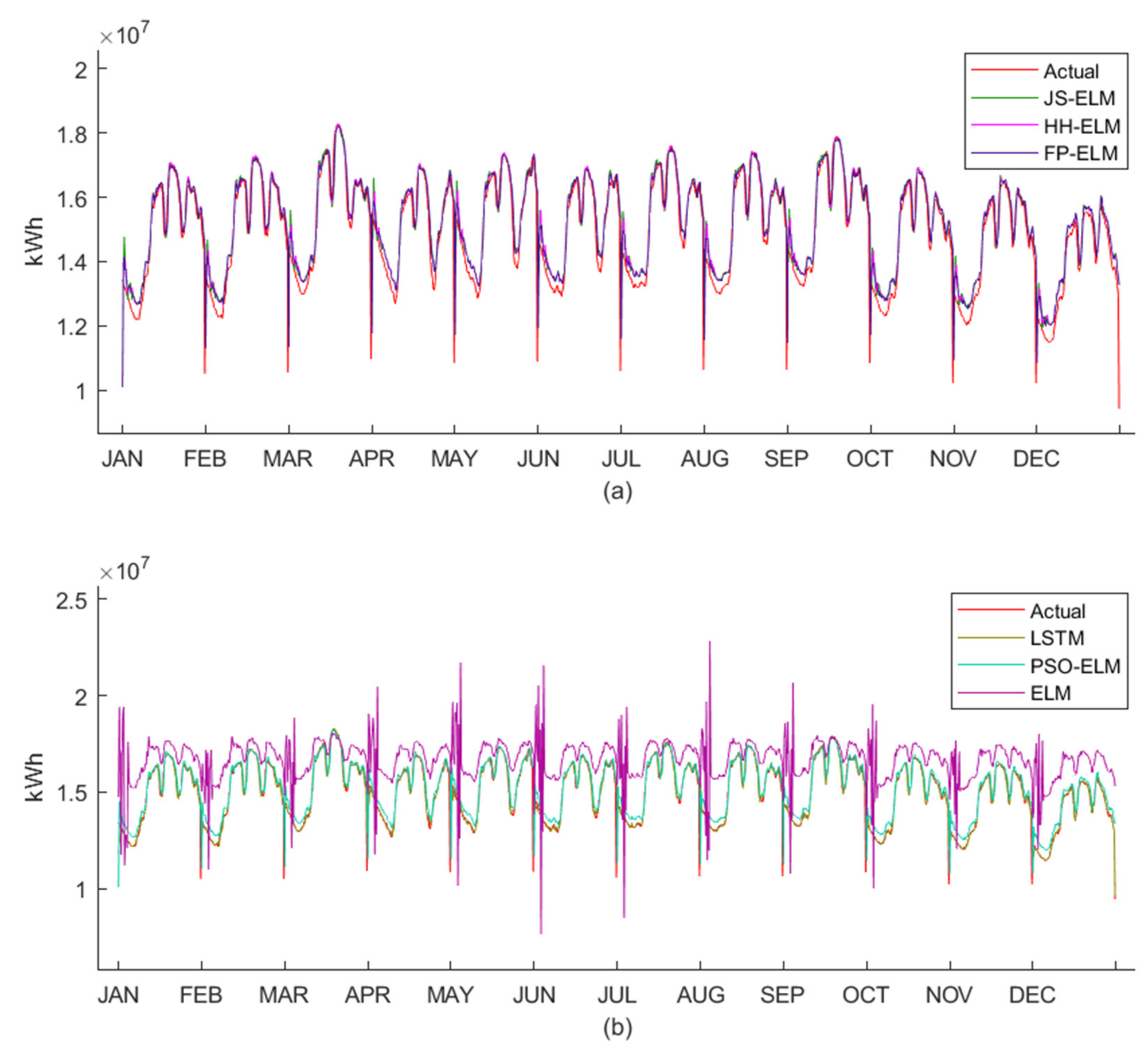
Figure 7a,b are the patterns of the peak demand data of electric energy and the pattern of the workday demand data of electric energy, respectively. Both peak demand data and workday demand data were collected in 15 min intervals from January 2018 to December 2020 in terms of a kiloWatt-Hour (kWh). The peak demand data were collected from the days that use the highest electricity for each month, and the workday demand data were collected from Monday to Friday for each month.
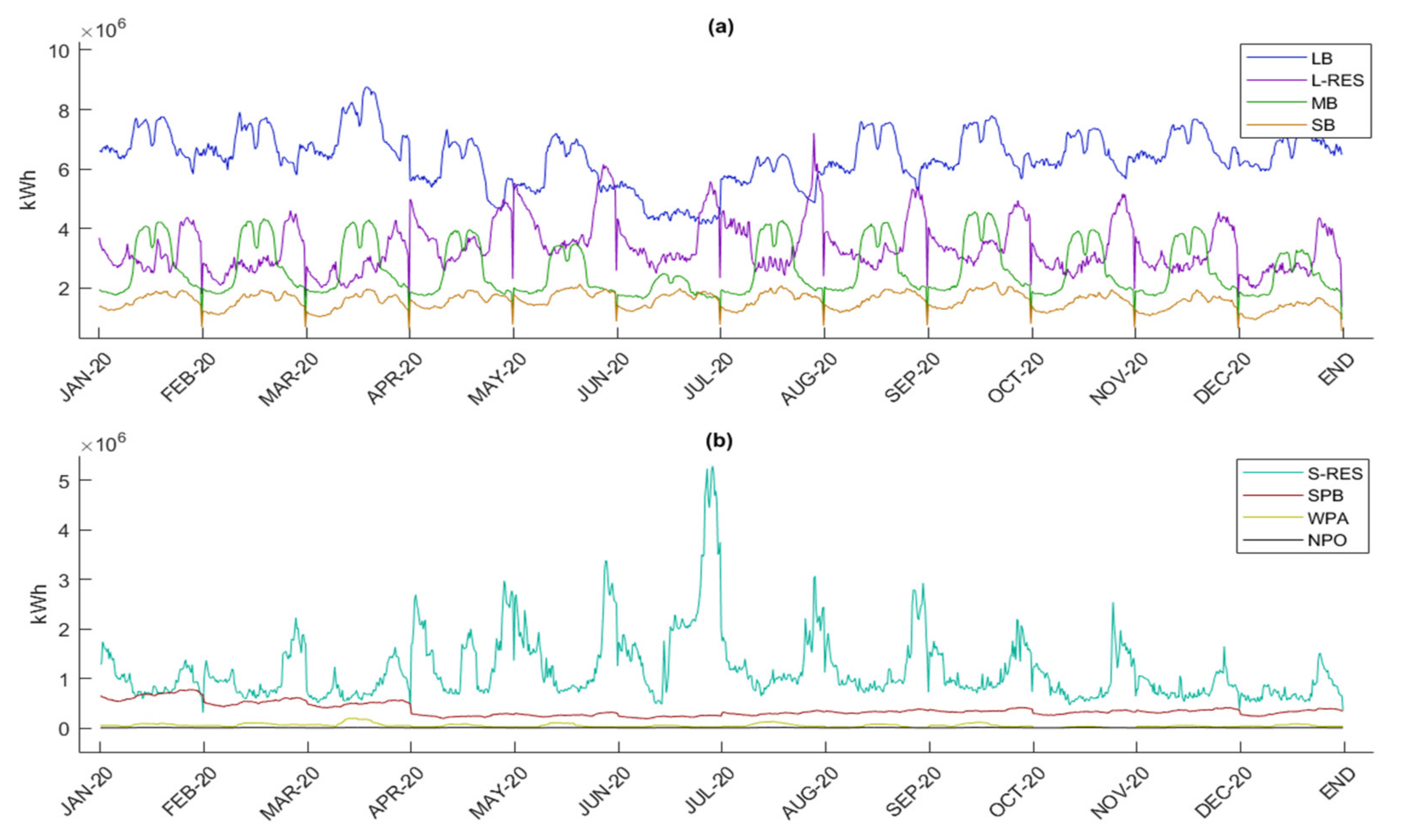
Figure 8 is the group pattern of the peak demand data of electric energy collected in 15 min intervals from January 2018 to December 2020 in terms of kWh. This dataset can be separated into 8 clusters when sorting from the highest total electric energy demand to the lowest total electric energy demand. The 8 clusters consist of Large Business (LB), Large Residential or Residential (L-RES) demand, which consumes energy greater than or equal to 150 kWh per month, Medium Business (MB), Small Business (SB), Small Residential or Residential (S-RES) demand, which consumes energy less than 150 kWh per month, Specific Business (SPB), Water Pumping for Agriculture (WPA), and Nonprofit Organization (NPO).

3.2. Dataset

When the preparation of electric energy demand data was completed, the experimental datasets were built to be tested in proposed models to forecast data with minimum error. In this research, the datasets were classified into seven groups for testing the proposed models. Table 2 describes the detail of each dataset, which is separated in terms of train and test data.
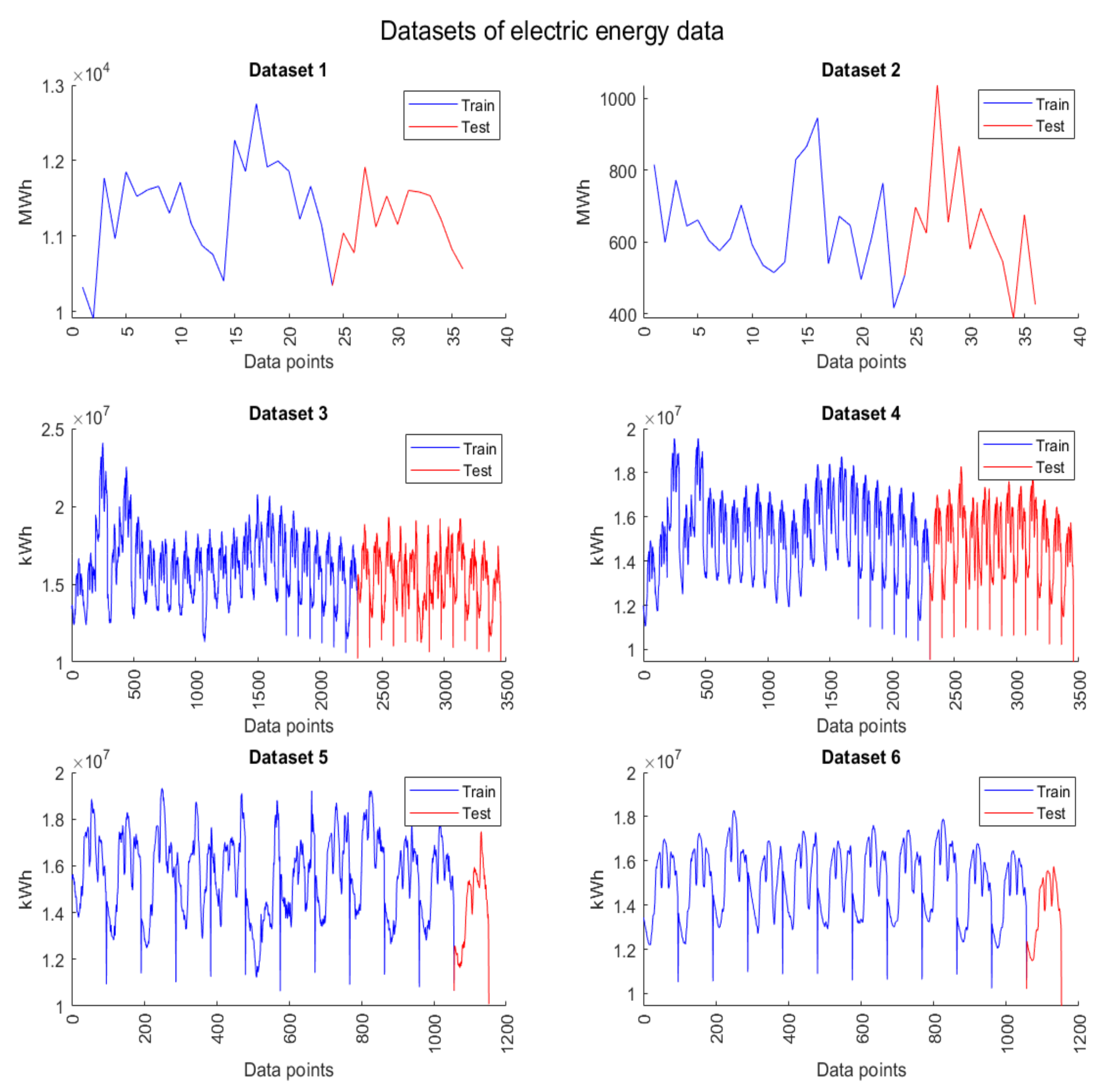
Figure 9 is the electric energy pattern data from dataset 1 to dataset 6, where the blue line is the train data for machine learning, and the red line is the test data for machine learning. Therefore, the detail from dataset 1 to dataset 6 can be described as follows:
Dataset 1 is the monthly electric energy demand data that is separated from January 2018 to December 2019 as train data (24 instances) and from January 2020 to December 2020 as test data (12 instances).
Dataset 2 is the monthly electric energy loss data that is separated from January 2018 to December 2019 as train data (24 instances) and from January 2020 to December 2020 as test data (12 instances).
Dataset 3 is the peak day 15 min interval electric energy demand data that is separated from January 2018 to December 2019 as train data (2304 instances) and from January 2020 to December 2020 as test data (1151 instances).
Dataset 4 is the workday 15 min interval electric energy demand data that is separated from January 2018 to December 2019 as train data (2304 instances) and from January 2020 to December 2020 as test data (1151 instances).
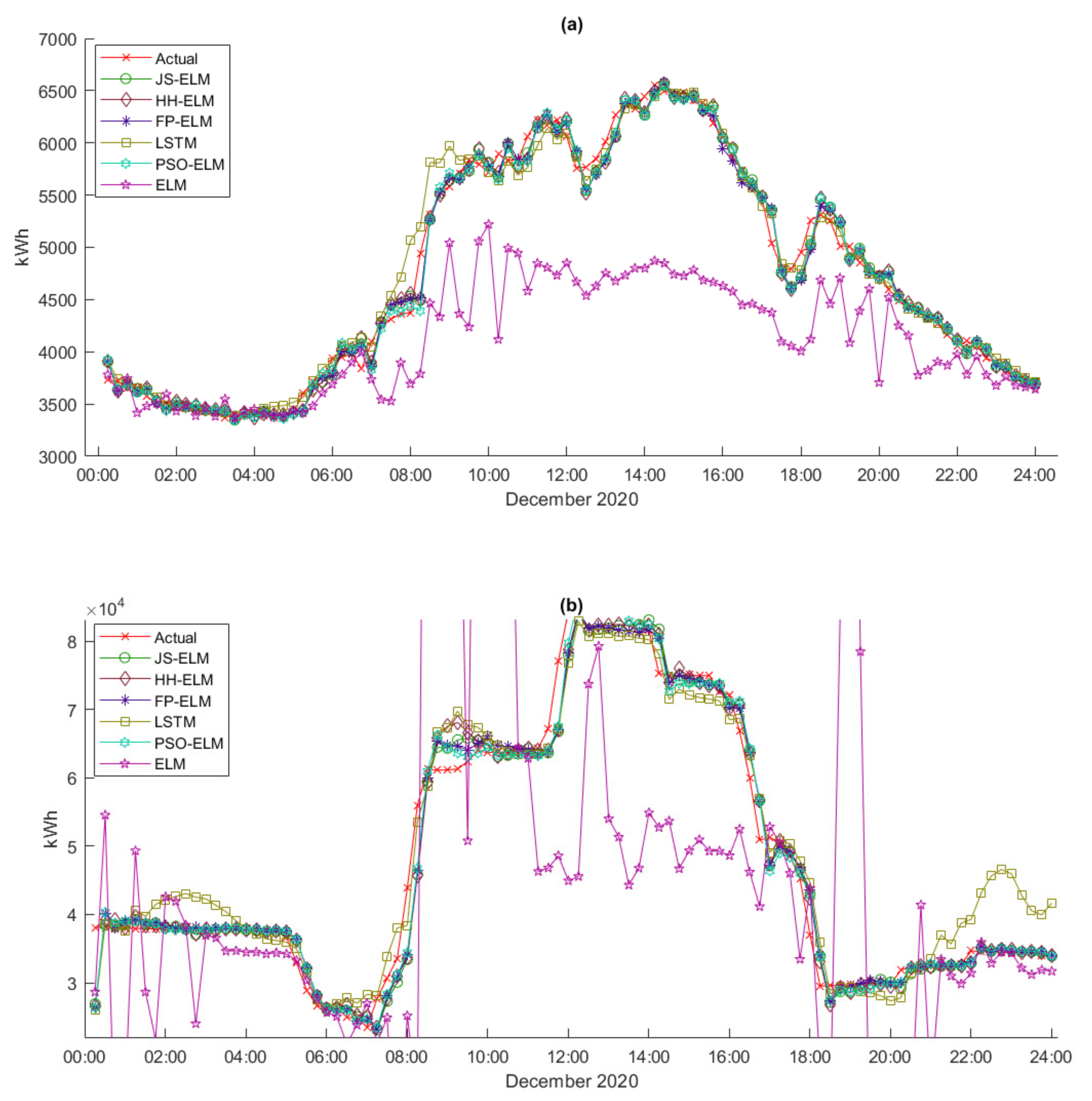
Dataset 5 is the peak day 15 min interval electric energy demand data that is separated from January 2020 to December 2020 as train data (1506 instances) and only December 2020 as test data (96 instances).
Dataset 6 is the workday 15 min interval electric energy demand data that is separated from January 2020 to December 2020 as train data (1506 instances) and only December 2020 as test data (96 instances).
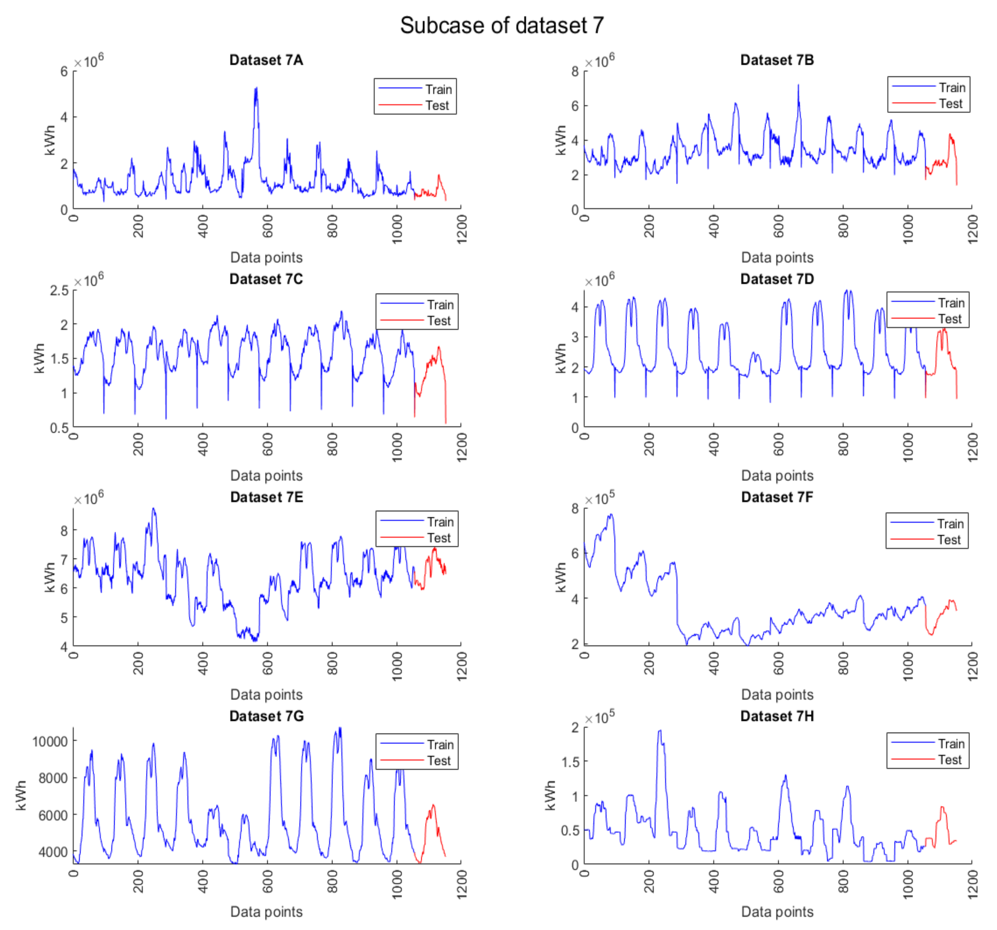
Figure 10 is the electric energy pattern data of dataset 7, where the blue line is the train data for machine learning, and the red line is the test data for machine learning. Therefore, the detail of dataset 7 can be described as follows:
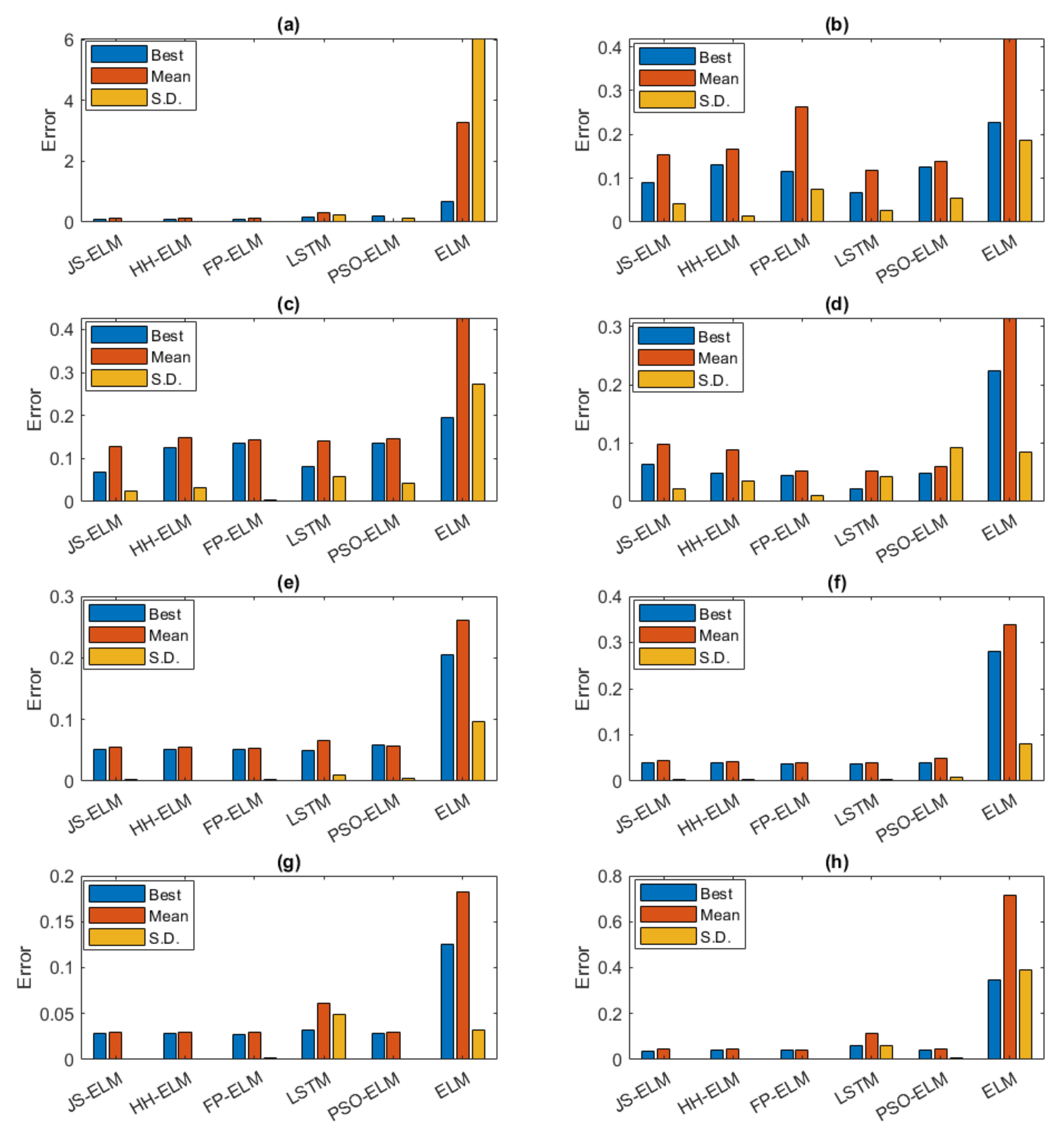
Dataset 7 is the cluster of 15 min interval peak day electric energy demand data that are separated into 8 subcases (7A to 7H). Subcase 7A is the cluster of S-RES electric energy demand data, subcase 7B is the cluster of L-RES electricity demand data, subcase 7C is the cluster of SB electricity demand data, subcase 7D is the cluster of MB electricity demand data, subcase 7E is the cluster of LB electricity demand data, subcase 7F is the cluster of SPB electricity demand data, subcase 7G is the cluster of NPO electricity demand data, and subcase 7H is the cluster of WPA electricity demand data. All subcases are separated from January 2020 to December 2020 as train data (1506 instances) and only December 2020 as test data (96 instances).

3.3. Proposed Models

The concept of the proposed models is using metaheuristic algorithms to optimize the weight parameter to reduce the cause of overfitting. In this research, three metaheuristic algorithms, which consist of JSO, HHO, and FPA, modified the randomization of weight parameter for searching the best weight parameter to improve the performance of the forecasting. The algorithm of the proposed models is described in Algorithm 1.
Algorithm 1. Pseudo-code of the Proposed Models.
1:Define objective function f(x), ( x i , t i )     R n   ×   R m by i = 1 , 2 , , N
2:Define the initialize n number of population in metaheuristic models (JSO, HHO, or FPA)
3:Define a switch probability p  ϵ [0,1] (FPA only)
4:Define the best solution g in the initial population
5:Define L hidden nodes in ELM
6:Define G w i , b i , x i Hidden nodes activation function in ELM (sigmoidal function)
7:Define β output weight vector
8:Define T as the max iteration for metaheuristic models
9:while (t < T)
10:  for i = 1: n
11:   Adjust w i t + 1 as the population with the metaheuristic models (JSO, HHO, or FPA)
12:   Evaluate new solution w i t + 1 to ELM
13:   for i = 1:L
14:    for j = 1:N
15:     H(i,j) =   G w i t + 1 , b i , x i β
16:    end
17:   end
18:   β = H T
19:  If new solutions are better, update new g in the population
20:    end for
21:Find the current best solution g & best output weight β
22:end while
First of all, based on the ELM model, all setting parameters were defined in the model, which consisted of a number of hidden nodes, input and target data, and initial weight parameter. Secondly, based on metaheuristic models, all setting parameters of each model were defined, which consisted of the number of populations, switch probability for the FPA model, and the best solution of the population. Thirdly, the weight parameter was defined based on metaheuristic models and then evaluated the new weight parameter for calculating in the ELM model. Fourthly, the activation function was calculated in the ELM model to receive the last weight parameter from the hidden layer. All processes were calculated until the iteration reached the max iteration criterion and the best weight parameter was received for calculating in the testing phase.

3.4. Experimental Setup and Hyper-Parameters Setting

The hardware specification of the computer used in this research work was CPU Intel Core i7-7700HQ 2.80 GHz (up to 3.40 GHz), RAM 32 GB, and SSD NVMe. The software was the MATLAB version R2020a. The major hyper-parameters [42,43] of proposed models consisted of the number of hidden nodes and the number of populations and the major hyper-parameters [44] of state-of-the-art models consisting of the number of hidden nodes that were analyzed through the electric energy demand datasets. The objective function to find the best hyper-parameters was the Root Mean Square Error (RMSE).
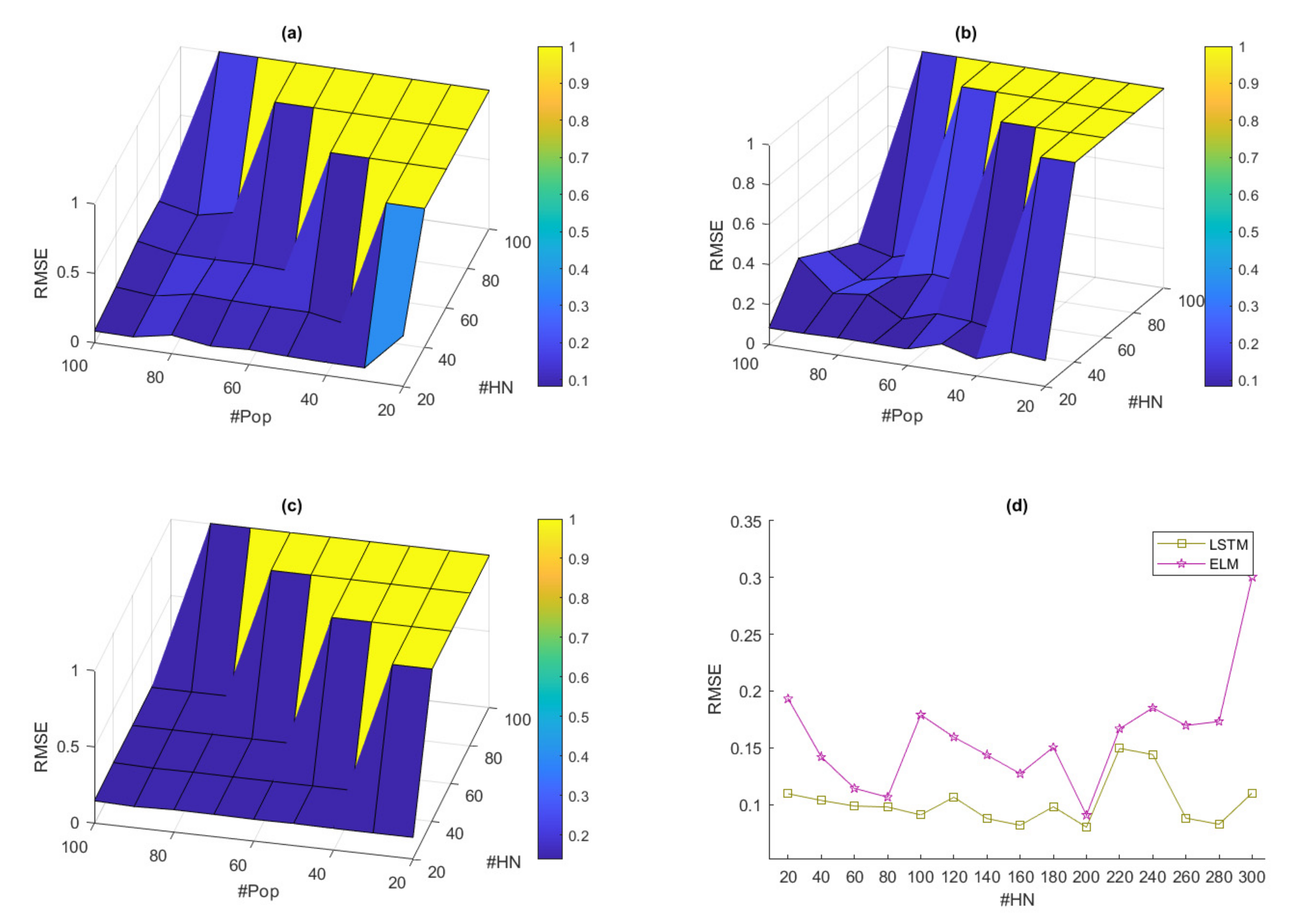
The hyper-parameter tuning [45,46] of the proposed and state-of-the-art models is shown in Figure 11. In this experiment, the average of RMSE from all models was obtained by taking all the datasets (7 datasets) used to find the RMSE value, then averaging RMSE value in terms of the number of hidden nodes and population. In the proposed models, the boundary of hidden nodes was set from 20 to 200 (increasing 20 nodes), the boundary of populations was set from 20 to 100 (increasing 10 populations), and the number of iterations for metaheuristics was set to 100 due to the fast computation. In the state-of-the-art models, the boundary of hidden nodes was set from 20 to 300 (increasing 20 nodes). For fast computing in the long short-term memory (LSTM) model, the fixed setting of hyper-parameters in the LSTM model consisted of 2 hidden layers, 1000 epochs, 64 batch size, and optimizer was set to Adam.
According to Figure 11, the hyper-parameter experiment results show that the best average RMSE of JS-ELM is 0.0838, and the locations of hidden nodes and populations are 40 and 50, respectively. The best average RMSE of HH-ELM is 0.0927, and the locations of hidden nodes and populations are 40 and 50, respectively. The best average RMSE of FP-ELM is 0.1384, and the locations of hidden nodes and populations are 40 and 50, respectively. The best average RMSE of LSTM is 0.0880, and the location of hidden nodes is 200. The best average RMSE of ELM is 0.0907, and the location of hidden nodes is 200.
For comparing with the metaheuristic-based proposed models, the Particle Swarm Optimization Extreme Learning Machine (PSO-ELM) [47,48] model was considered to forecast in electric energy demand datasets. The best hyper-parameters of PSO-ELM model were received from [48], which consist of 150 hidden nodes, 30 populations (swarm size), acceleration coefficients C 1 = 1 and C 2 = 2 , and inertia weight was set to 0.9.
To summarize, the best hyper-parameters of JS-ELM, HH-ELM, and FP-ELM are 40 hidden nodes and 50 populations. The best hyper-parameters of LSTM and ELM are 200 hidden nodes. All suitable hyper-parameters were defined as presented in Table 3.

3.5. Performance Evaluation

In this research, all datasets were processed by min–max normalization [49] as calculated in (25).
x = x min x max x min x
where x is a data point and x is normalized data.
To evaluate the performance of proposed models, three error metrics, Mean Absolute Error (MAE), Mean Absolute Percentage Error (MAPE), and Root Mean Square Error (RMSE), were used in this experiment as presented in (26)–(28), respectively.
M A E t = 1 n i = 1 n e i t i
M A P E t = 100 n i = 1 n e i t i t i
R M S E t = i = 1 n e i t i 2 n
where i is the present time variable, n is the number of input data, e i is the expected data at the time i, and t i is the actual data at the time i.
To receive the best solution from the performance evaluation, which is suggested from [50,51], all error metrics were combined to the Cumulative Weighted Error (CWE) for evaluating the final result of the experiment as presented in (29).
C W E = M A E + M A P E 100 + R M S E 3
After error metrics were completely calculated, the result of error metrics was used to evaluate the performance of the proposed models as discussed in Section 4.

4. Experimental Results

This section describes the experimental results of the proposed models and ELM using electric energy demand datasets. This section is separated into three subsections consisting of the experimental results overview, forecasting time consumption for each model, and the summary of the experimental results.

4.1. Discussion of the Experimental Results

In the experimental results, the datasets mentioned in Section 3.2 were set. The forecasting error of the proposed models was presented and all error metrics as mentioned in Section 3.5 were compared. According to Table 4, the detail of the experimental result is described in terms of the dataset with the minimum error, minimum mean error, and standard deviation (S.D.) error result when using the number of global iterations defined in Table 3.
The minimum error was obtained by finding the lowest forecasting error result from the global iterations as presented in (30). The minimum mean error was obtained by averaging all results from the global iterations as presented in (31). The minimum S.D. error was obtained by using the forecasting error result and the minimum mean error result to indicate the standard deviation of the error solution from global iterations as presented in (32).
E = min i E i i = 1 N
μ = 1 N i = 1 N E i
σ = 1 N 1 i = 1 N E i μ 2
where E is the minimum error, μ is the minimum mean error, σ is the minimum S.D. error, i is the present time variable, N is the number of global iterations, and E i is the result of the forecasting error metric for each global iteration.
The minimum forecasting error result of dataset 1 is shown in Figure 12. The result shows that all models provided results near the actual target value. Furthermore, according to the CWE error metric in Table 4, JS-ELM provided the best minimum error result when compared to the other models’ results. However, LSTM, PSO-ELM, and ELM provided higher stability of forecasting when considered on the minimum mean error and minimum S.D. error. HH-ELM provided the minimum error lower than that of the ELM model, but the minimum mean error was higher than that of the ELM model. The overall error metrics of FP-ELM were higher than those of other models.
The minimum forecasting error result of dataset 2 is shown in Figure 13. The result shows that all models provided results near the actual target value. Furthermore, according to the CWE error metric in Table 4, JS-ELM provided the best minimum error result when compared to the other models’ results. However, the minimum mean error and minimum standard deviation of JS-ELM, HH-ELM, FP-ELM, and PSO-ELM were higher than those of the LSTM and ELM models, which means the proposed models could provide the instability of the attempt to dataset 2.
The minimum forecasting error result of dataset 3 s shown in Figure 14. All proposed models and LSTM provided results near the actual target value. The ELM model was already overfitted because the training RMSE result was 0.0207, but the forecasting RMSE result was 0.1668. Furthermore, the minimum mean error and minimum standard deviation of ELM were higher than those of the proposed models, which means the ELM could provide the instability of the attempt to dataset 3.
The minimum forecasting error result of dataset 4 is shown in Figure 15. All proposed models and LSTM provided results near the actual target value. The ELM model was already overfitted because the training RMSE result was 0.0253, but the forecasting RMSE result was 0.1504. Furthermore, the minimum mean error and minimum standard deviation of ELM were higher than those of proposed models, which means the ELM could provide the instability of the attempt to dataset 4.
The minimum forecasting error result of dataset 5 is shown in Figure 16. The result shows that the expected target value of JS-ELM was close to the actual target value. The expected target values of HH-ELM and FP-ELM slightly swung from 02:00 to 04:00 when compared to the actual target value. The expected target values of LSTM slightly swung from 00:00 to 01:00 when compared to the actual target value. The expected target value of ELM was clearly different from the actual target value.
The minimum forecasting error result of dataset 6 is shown in Figure 17. The result shows that all models provided results near the actual target value. However, the ELM model was already overfitted because the training RMSE result was 0.0151, but the forecasting RMSE result was 0.2347. Furthermore, the minimum mean error and minimum standard deviation of ELM were higher than those of the proposed models, which means ELM could provide the instability of the attempt to dataset 6.
The minimum forecasting error results of dataset 7 are shown in Figure 18, Figure 19 and Figure 20. Dataset 7 contained eight sub-datasets to attempt on this experiment, which consists of sub-dataset 7A (the S-RES profile), sub-dataset 7B (the L-RES profile), sub-dataset 7C (the SB profile), sub-dataset 7D (the MB profile), sub-dataset 7E (the LB profile), sub-dataset 7F (the SPB profile), sub-dataset 7G (the NPO profile), and sub-dataset 7H (the WPA profile). The overall results of dataset 7 show that the proposed models provided the results nearest to the actual target value. However, the expected target value of the ELM model was instability, which means the ELM model was already overfitted because the training accuracy between the expected target value and actual target value was overrated, thus, the forecasting result was unacceptable. Furthermore, the minimum mean error and minimum standard deviation of ELM were higher than those of the proposed models, which means the ELM could provide the instability of the attempt to dataset 7.

4.2. Discussion on the Time Consumption

In this research, the training times of each forecasting model were calculated and compared. According to Table 5, the result of the training time showed that ELM consumed the least time compared with other models. Due to the metaheuristic calculation, JS-ELM and FP-ELM consumed a lower amount of time to calculate the data and provide the best result. HH-ELM consumed more time than the other models because the number of time steps of the HHO calculation are greater than JSO and FPA. However, the LSTM model consumed more time than all other models in the experiment. The forecasting time was not focused upon because all models consumed a low forecasting time (in milliseconds).

4.3. Summary of the Experimental Results

In this research, three main factors, the minimum error, minimum mean error, and minimum standard deviation, were analyzed by error metrics (MAE, MAPE, RMSE, and CWE) to evaluate the performance of all models that fitted each dataset.
The CWE comparison for all models from datasets 1 to 6 is shown in Figure 21. For datasets 1 and 2, the JS-ELM model was the most suitable in terms of the minimum error result, while the ELM was the most suitable in terms of the minimum mean error and S.D. error. For dataset 3, the FP-ELM model was suitable for all three factors. For dataset 4, the LSTM model was the most suitable in terms of the minimum error result, while the FP-ELM was the most suitable in terms of the minimum mean error and S.D. error. For datasets 5 and 6, the JS-ELM model was the most suitable in terms of the minimum error result, while HH-ELM and FP-ELM were the most suitable in terms of the minimum mean error and S.D. error, respectively.
The CWE comparison of all models for dataset 7 is shown in Figure 22. All proposed models were the most suitable for all three factors, while the ELM model provided the highest CWE rate, which means the ELM model was already overfitted, as referred to in Section 4.1.
According to Section 4.2, the time consumptions of the proposed models were higher than the time consumption of the ELM model because the proposed models were tuned by metaheuristics optimization. Major factors that directly affected the high time consumption of the proposed models consist of the time step calculation for each metaheuristic algorithm, number of populations, iterations of the metaheuristics algorithms, and number of hidden nodes of the ELM model. In conclusion, the proposed models slightly consumed more time in calculation than the time consumption of the ELM model, while the experiment results for all datasets were highly accurate and more stable than the result of the ELM model.
In comparison, the overall error results of the proposed models and LSTM were close. However, according to Table 5, the training time of the proposed models was faster than the LSTM model.

5. Conclusions and Future Work

This research proposed the novel ELM model optimized by metaheuristic algorithms, namely JS-ELM, HH-ELM, and FP-ELM, to forecast the electric energy dataset. The characteristic of the metaheuristic optimizations, namely JSO, HHO, and FPA, is that they are self-adaptive to tune the weight parameter of the ELM model without being trapped in the local optimum. Therefore, the models mentioned earlier were applied to the ELM model by tuning the weight parameter of the ELM model instead of using the traditional randomization of the weight parameter. In addition, these three optimization methods can reduce the number of hidden nodes of the ELM model. To demonstrate the performance of the proposed method, all models were applied to forecast seven real-life electric energy datasets. The dataset of electric energy demand consists of monthly electric energy demand data from 2018 to 2020, monthly electric energy loss data from 2018 to 2020, peak day 15 min interval electric energy demand data from 2018 to 2020, workday 15 min interval electric energy demand data from 2018 to 2020, peak day 15 min interval electric energy demand data in 2020, workday 15 min interval electric energy demand data in 2020, and cluster of 15 min interval peak day electric energy demand data. Consequently, the result showed that the proposed models could improve the forecasting accuracy, provide forecasting stability, and reduce the cause of overfitting from the traditional model.
According to Table 6, the JS-ELM model was the most suitable for the minimum error result. The overall forecasting results of the HH-ELM model were similar to the JS-ELM model results, but the time consumption was higher than the time consumption of other models. The FP-ELM model was the most suitable in terms of the minimum mean error and minimum S.D. The time consumption of the proposed models depended on the number of populations, iterations criterion of metaheuristics algorithms, and the number of hidden nodes of the ELM model. The HH-ELM model used twice the time consumption compared with the time consumptions of the JS-ELM and the FP-ELM models. Furthermore, the time consumptions of the proposed models were lower than the LSTM model, while the overall error results of the proposed models and LSTM were close.
For suggestions for future works, the proposed models can improve the stability of forecasting, for instance, according to Table 6, JS-ELM was the most suitable when considering the minimum error result, and FP-ELM was the most suitable when considering the S.D. result. Therefore, future work may propose a novel model that applies the hybrids of JSO and FPA to the ELM model. Due to the benefits of JSO and FPA, the expected results of the aforementioned novel model can be achieved with a more stable accuracy of forecasting and provide the best forecasting result. Moreover, the time consumption of forecasting is the major topic to discuss. According to Table 5, the time consumption of JS-ELM and FP-ELM were close and less than other models except for ELM. The time consumption of the proposed models and the future novel model can be reduced by using the step of tuning the hyper-parameters with a suitable algorithm and the methodology of an ensemble learning algorithm [52,53,54] that splits the appropriate sub-datasets from the primary dataset, forecasts the sub-datasets, and aggregates the forecasted model results. Finally, due to the variety of metaheuristics algorithms [47] that are continuously being developed, an alternative metaheuristics algorithm can be discussed to implement with the ELM model or other machine learning models to improve the accuracy of the forecasted electric energy demand.

Author Contributions

S.B.: writing—original draft preparation, conceptualization, methodology, software, data curation, simulation. C.S.: supervision, investigation, conceptualization, writing—review and editing. P.F.: supervision, investigation, conceptualization, data curation, resources. R.C.: supervision, writing—review and editing, formal analysis, methodology, investigation, validation. All authors have read and agreed to the published version of the manuscript.

Funding

This work was supported by the Provincial Electricity Authority of Thailand, which provided funding and useful information for the experiment in this research, and the Faculty of Engineering, Khon Kaen University, under Grant Ph.D.Ee-1/2564.

Institutional Review Board Statement

Not applicable.

Informed Consent Statement

Not applicable.

Data Availability Statement

Datasets from Section 3 (electric energy demand data) can be found and downloaded at http://peaoc.pea.co.th/loadprofile/en/. (accessed on 8 October 2021).

Conflicts of Interest

The authors declare that they have no known competing financial interests or personal relationships that could have appeared to influence the work reported in this paper.

References

  1. Pritima, D.; Krishnan, P.G.; Padmanabhan, P.; Stalin, B. Performance of electrical energy based unconventional machining processes—Review. Mater. Today Proc. 2021, in press. [Google Scholar] [CrossRef]
  2. Hyndman, R.J. Forecasting: An Overview. In International Encyclopedia of Statistical Science; Springer: Berlin/Heidelberg, Germany, 2011; pp. 536–539. [Google Scholar] [CrossRef]
  3. Mas-Machuca, M.; Sainz, M.; Martinez-Costa, C. A review of forecasting models for new products. Intang. Cap. 2014, 10, 1–25. [Google Scholar] [CrossRef] [Green Version]
  4. Palm, F.C.; Nijman, T.E. Missing Observations in the Dynamic Regression Model. Econometrica 1984, 52, 1415. [Google Scholar] [CrossRef] [Green Version]
  5. Box, G.E.P.; Jenkins, G.M.; Reinsel, G.C.; Ljung, G.M. Time Series Analysis: Forecasting and Control, 5th ed.; John Wiley & Sons: Hoboken, NJ, USA, 2015. [Google Scholar]
  6. Brown, R.G. Smoothing, Forecasting and Prediction of Discrete Time Series; Prentice-Hall: Englewood Cliffs, NJ, USA, 1963. [Google Scholar]
  7. Mcculloch, W.S.; Pitts, W.H. A logical calculus of the ideas immanent in nervous activity. Bull. Math. Biophys. 1943, 5, 115–133. [Google Scholar] [CrossRef]
  8. Memarzadeh, G.; Keynia, F. Short-term electricity load and price forecasting by a new optimal LSTM-NN based prediction algorithm. Electr. Power Syst. Res. 2020, 192, 106995. [Google Scholar] [CrossRef]
  9. Liu, Z.; Loo, C.K.; Pasupa, K. A novel error-output recurrent two-layer extreme learning machine for multi-step time series prediction. Sustain. Cities Soc. 2020, 66, 102613. [Google Scholar] [CrossRef]
  10. Larrea, M.; Porto, A.; Irigoyen, E.; Barragán, A.J.; Andújar, J.M. Extreme learning machine ensemble model for time series forecasting boosted by PSO: Application to an electric consumption problem. Neurocomputing 2020, 452, 465–472. [Google Scholar] [CrossRef]
  11. Chen, Y.; Kloft, M.; Yang, Y.; Li, C.; Li, L. Mixed kernel based extreme learning machine for electric load forecasting. Neurocomputing 2018, 312, 90–106. [Google Scholar] [CrossRef]
  12. Chen, Q.; Xia, M.; Lu, T.; Jiang, X.; Liu, W.; Sun, Q. Short-Term Load Forecasting Based on Deep Learning for End-User Transformer Subject to Volatile Electric Heating Loads. IEEE Access 2019, 7, 162697–162707. [Google Scholar] [CrossRef]
  13. Rafi, S.H.; Masood, N.A.; Deeba, S.R.; Hossain, E. A Short-Term Load Forecasting Method Using Integrated CNN and LSTM Network. IEEE Access 2021, 9, 32436–32448. [Google Scholar] [CrossRef]
  14. Sajjad, M.; Khan, Z.A.; Ullah, A.; Hussain, T.; Ullah, W.; Lee, M.Y.; Baik, S.W. A Novel CNN-GRU-Based Hybrid Approach for Short-Term Residential Load Forecasting. IEEE Access 2020, 8, 143759–143768. [Google Scholar] [CrossRef]
  15. Hu, Y.; Li, J.; Hong, M.; Ren, J.; Lin, R.; Liu, Y.; Liu, M.; Man, Y. Short term electric load forecasting model and its verification for process industrial enterprises based on hybrid GA-PSO-BPNN algorithm—A case study of papermaking process. Energy 2019, 170, 1215–1227. [Google Scholar] [CrossRef]
  16. Kazemzadeh, M.-R.; Amjadian, A.; Amraee, T. A hybrid data mining driven algorithm for long term electric peak load and energy demand forecasting. Energy 2020, 204, 117948. [Google Scholar] [CrossRef]
  17. Hafeez, G.; Alimgeer, K.S.; Khan, I. Electric load forecasting based on deep learning and optimized by heuristic algorithm in smart grid. Appl. Energy 2020, 269, 114915. [Google Scholar] [CrossRef]
  18. Huang, G.-B.; Zhu, Q.-Y.; Siew, C.-K. Extreme learning machine: Theory and applications. Neurocomputing 2006, 70, 489–501. [Google Scholar] [CrossRef]
  19. Penrose, R. A generalized inverse for matrices. Math. Proc. Camb. Philos. Soc. 1955, 51, 406–413. [Google Scholar] [CrossRef] [Green Version]
  20. Wang, J.; Lu, S.; Wang, S.-H.; Zhang, Y.-D. A review on extreme learning machine. Multimedia Tools Appl. 2021, 80, 1–50. [Google Scholar] [CrossRef]
  21. Horata, P.; Chiewchanwattana, S.; Sunat, K. Robust extreme learning machine. Neurocomputing 2013, 102, 31–44. [Google Scholar] [CrossRef]
  22. Song, S.; Wang, M.; Lin, Y. An improved algorithm for incremental extreme learning machine. Syst. Sci. Control Eng. 2020, 8, 308–317. [Google Scholar] [CrossRef]
  23. Chou, J.-S.; Truong, D.-N. A novel metaheuristic optimizer inspired by behavior of jellyfish in ocean. Appl. Math. Comput. 2020, 389, 125535. [Google Scholar] [CrossRef]
  24. Heidari, A.A.; Mirjalili, S.; Faris, H.; Aljarah, I.; Mafarja, M.; Chen, H. Harris hawks optimization: Algorithm and applications. Futur. Gener. Comput. Syst. 2019, 97, 849–872. [Google Scholar] [CrossRef]
  25. Yang, X.-S. Flower Pollination Algorithm for Global Optimization. In Lecture Notes in Computer Science (Including Subseries Lecture Notes in Artificial Intelligence and Lecture Notes in Bioinformatics); Springer: Berlin/Heidelberg, Germany, 2012; Volume 7445, pp. 240–249. Available online: https://0-doi-org.brum.beds.ac.uk/10.1007/978-3-642-32894-7_27 (accessed on 16 June 2021).
  26. Hyndman, R.J.; Athanasopoulos, G. Forecasting: Principles and Practice, 3rd ed.; OTexts: Melbourne, Australia, 2021; Available online: https://otexts.com/fpp3/index.html (accessed on 10 February 2021).
  27. Armstrong, J.S.; Green, K.C. Forecasting methods and principles: Evidence-based checklists. J. Glob. Sch. Mark. Sci. 2018, 28, 103–159. [Google Scholar] [CrossRef]
  28. Mohamad, M.; Selamat, A.; Subroto, I.M.; Krejcar, O. Improving the classification performance on imbalanced data sets via new hybrid parameterisation model. J. King Saud Univ. Comput. Inf. Sci. 2019, 33, 787–797. [Google Scholar] [CrossRef]
  29. Dinh, D.-T.; Huynh, V.-N.; Sriboonchitta, S. Clustering mixed numerical and categorical data with missing values. Inf. Sci. 2021, 571, 418–442. [Google Scholar] [CrossRef]
  30. Millsap, R.E.; Chase, C.W.J. R: A Language and Environment for Statistical Computing. J. Bus. Forecast. Methods Syst. 1995, 14, 461–473. Available online: http://www.r-project.org (accessed on 12 July 2021).
  31. Boriratrit, S.; Tepsiri, W.; Krobnopparat, A.; Khunsaeng, N. Forecasting and Evaluation Electricity Loss in Thailand via Flower Pollination Extreme Learning Machine Model. In Proceedings of the 2018 IEEE International Conference on Smart Energy Grid Engineering (SEGE), Oshawa, ON, Canada, 12–15 August 2018; pp. 160–164. [Google Scholar] [CrossRef]
  32. Bastian, T.; Lilley, M.K.; Beggs, S.E.; Hays, G.C.; Doyle, T.K. Ecosystem relevance of variable jellyfish biomass in the Irish Sea between years, regions and water types. Estuar. Coast. Shelf Sci. 2014, 149, 302–312. [Google Scholar] [CrossRef]
  33. May, R.M. Simple mathematical models with very complicated dynamics. Nature 1976, 261, 459–467. [Google Scholar] [CrossRef]
  34. Bednarz, J.C. Cooperative Hunting Harris’ Hawks (Parabuteo unicinctus). Science 1988, 239, 1525–1527. [Google Scholar] [CrossRef]
  35. Kleinberg, J.M. Navigation in a small world. Nature 2000, 406, 845. [Google Scholar] [CrossRef]
  36. Gomes, W.; Beck, A.; Lopez, R.H.; Miguel, L.F. A probabilistic metric for comparing metaheuristic optimization algorithms. Struct. Saf. 2018, 70, 59–70. [Google Scholar] [CrossRef]
  37. Kaul, S.; Kumar, Y. Nature-Inspired Metaheuristic Algorithms for Constraint Handling: Challenges, Issues, and Research Perspective. In Constraint Handling in Metaheuristics and Applications; Springer: Singapore, 2021; pp. 55–80. [Google Scholar] [CrossRef]
  38. Alabool, H.M.; Alarabiat, D.; Abualigah, L.; Heidari, A.A. Harris hawks optimization: A comprehensive review of recent variants and applications. Neural Comput. Appl. 2021, 33, 8939–8980. [Google Scholar] [CrossRef]
  39. Lei, M.; Zhou, Y.; Luo, Q. Enhanced Metaheuristic Optimization: Wind-Driven Flower Pollination Algorithm. IEEE Access 2019, 7, 111439–111465. [Google Scholar] [CrossRef]
  40. PEA. Load Profile: Load Research of PEA. Available online: http://peaoc.pea.co.th/loadprofile/en/ (accessed on 2 August 2021).
  41. PEA. Electricity Sales Report & Load Research of PEA. Provincial Electricity Authority of Thailand. 2020. Available online: http://peaoc.pea.co.th/ (accessed on 8 October 2021).
  42. Shahhosseini, M.; Hu, G.; Pham, H. Optimizing ensemble weights and hyperparameters of machine learning models for regression problems. Mach. Learn. Appl. 2022, 7, 100251. [Google Scholar] [CrossRef]
  43. Agrawal, T. Hyperparameter Optimization in Machine Learning; Apress: Berkeley, CA, USA, 2021; volume XIX, p. 166. Available online: https://0-doi-org.brum.beds.ac.uk/10.1007/978-1-4842-6579-6 (accessed on 29 November 2021).
  44. Nakisa, B.; Rastgoo, M.N.; Rakotonirainy, A.; Maire, F.; Chandran, V. Long Short Term Memory Hyperparameter Optimization for a Neural Network Based Emotion Recognition Framework. IEEE Access 2018, 6, 49325–49338. [Google Scholar] [CrossRef]
  45. Xie, Y.; Li, C.; Tang, G.; Liu, F. A novel deep interval prediction model with adaptive interval construction strategy and automatic hyperparameter tuning for wind speed forecasting. Energy 2020, 216, 119179. [Google Scholar] [CrossRef]
  46. Neshat, M.; Nezhad, M.M.; Abbasnejad, E.; Mirjalili, S.; Groppi, D.; Heydari, A.; Tjernberg, L.B.; Garcia, D.A.; Alexander, B.; Shi, Q.; et al. Wind turbine power output prediction using a new hybrid neuro-evolutionary method. Energy 2021, 229, 120617. [Google Scholar] [CrossRef]
  47. Mirjalili, S. Projects, Seyedali Mirjalili Project. 2022. Available online: https://seyedalimirjalili.com/projects (accessed on 15 March 2022).
  48. Kaloop, M.R.; Kumar, D.; Samui, P.; Gabr, A.R.; Hu, J.W.; Jin, X.; Roy, B. Particle Swarm Optimization Algorithm-Extreme Learning Machine (PSO-ELM) Model for Predicting Resilient Modulus of Stabilized Aggregate Bases. Appl. Sci. 2019, 9, 3221. [Google Scholar] [CrossRef] [Green Version]
  49. Patro, S.G.K.; Sahu, K.K. Normalization: A preprocessing stage. Int. Adv. Res. J. Sci. Eng. Technol. 2015, 2, 20–22. [Google Scholar] [CrossRef]
  50. Pirbazari, A.M.; Farmanbar, M.; Chakravorty, A.; Rong, C. Short-Term Load Forecasting Using Smart Meter Data: A Generalization Analysis. Processes 2020, 8, 484. [Google Scholar] [CrossRef]
  51. Asare-Bediako, B.; Kling, W.L.; Ribeiro, P.F. Day-ahead residential load forecasting with artificial neural networks using smart meter data. In Proceedings of the 2013 IEEE Grenoble Conference, Grenoble, France, 16–20 June 2013; pp. 1–6. [Google Scholar] [CrossRef]
  52. Wijaya, D.R.; Afianti, F.; Arifianto, A.; Rahmawati, D.; Kodogiannis, V.S. Ensemble machine learning approach for electronic nose signal processing. Sens. Bio-Sens. Res. 2022, 36, 100495. [Google Scholar] [CrossRef]
  53. Carneiro, T.C.; Rocha, P.A.; Carvalho, P.C.; Fernández-Ramírez, L.M. Ridge regression ensemble of machine learning models applied to solar and wind forecasting in Brazil and Spain. Appl. Energy 2022, 314, 118936. [Google Scholar] [CrossRef]
  54. Matrenin, P.; Safaraliev, M.; Dmitriev, S.; Kokin, S.; Ghulomzoda, A.; Mitrofanov, S. Medium-term load forecasting in isolated power systems based on ensemble machine learning models. Energy Rep. 2021, 8, 612–618. [Google Scholar] [CrossRef]
Figure 1. Overview of the Basic Forecasting Process [26].
Computers 11 00066 g001
Figure 2. The architecture of the Extreme Learning Machine Model [18,31].
Computers 11 00066 g002
Figure 3. Flowchart of the Jellyfish Search Optimization [23].
Computers 11 00066 g003
Figure 4. Flowchart of the Harris Hawk Optimization [24].
Computers 11 00066 g004
Figure 5. Flowchart of the Flower Pollination Algorithm [25].
Computers 11 00066 g005
Figure 6. (a) The pattern of electric energy demand data from 2018 to 2020. (b) The pattern of electric energy loss data from 2018 to 2020.
Computers 11 00066 g006
Figure 7. (a) Pattern of peak day electric energy demand data from 2018 to 2020. (b) Pattern of workday electric energy demand data from 2018 to 2020.
Computers 11 00066 g007
Figure 8. (a) Pattern of high electric energy demand cluster, which consists of Large Business (LB), Large Residential (L-RES), Medium Business (MB), and Small Business (SB). (b) Pattern of low electric energy demand cluster, which consists of Small Residential (S-RES), Specific Business (SPB), Water Pumping for Agriculture (WPA), and Nonprofit Organization (NPO).
Computers 11 00066 g008
Figure 9. Train data (blue line) and test data (red line) of datasets 1 to 6 [40,41].
Computers 11 00066 g009
Figure 10. Train data (blue line) and test data (red line) of each subcase of dataset 7 [40,41].
Computers 11 00066 g010
Figure 11. Hyper-parameter tuning of the proposed and state-of-the-art models where #pop is the number of populations and #HN is the number of hidden nodes. (a) The average RMSE of JS-ELM. (b) The average RMSE of HH-ELM. (c) The average RMSE of FP-ELM. (d) The average RMSE of LSTM and ELM.
Computers 11 00066 g011
Figure 12. Forecasting result of dataset 1 (minimum error result).
Computers 11 00066 g012
Figure 13. Forecasting result of dataset 2 (minimum error result).
Computers 11 00066 g013
Figure 14. Forecasting result of dataset 3 (minimum error result). (a) Forecasted energy of each proposed model. (b) Forecasted energy of each state-of-the-art model.
Computers 11 00066 g014
Figure 15. Forecasting result of dataset 4 (minimum error result). (a) Forecasted energy of each proposed model. (b) Forecasted energy of each state-of-the-art model.
Computers 11 00066 g015
Figure 16. Forecasting result of dataset 5 (minimum error result). (a) Forecasted energy of each proposed model. (b) Forecasted energy of each state-of-the-art model.
Computers 11 00066 g016
Figure 17. Forecasting result of dataset 6 (minimum error result). (a) Forecasted energy of each proposed model. (b) Forecasted energy of each state-of-the-art model.
Computers 11 00066 g017
Figure 18. Forecasting result of dataset 7A–7C (minimum error result). (a) Forecasted energy of each proposed model in dataset 7A. (b) Forecasted energy of each proposed model in dataset 7B. (c) Forecasted energy of each proposed model in dataset 7C.
Computers 11 00066 g018
Figure 19. Forecasting result of dataset 7D–7F (minimum error result). (a) Forecasted energy of each proposed model in dataset 7D. (b) Forecasted energy of each proposed model in dataset 7E. (c) Forecasted energy of each proposed model in dataset 7F.
Computers 11 00066 g019
Figure 20. Forecasting result of dataset 7G–7H (minimum error result). (a) Forecasted energy of each proposed model in dataset 7G. (b) Forecasted energy of each proposed model in dataset 7H.
Computers 11 00066 g020
Figure 21. CWE comparison for all models from datasets 1 to 6 (lower is better). (a) CWE comparison of each proposed model in dataset 1. (b) CWE comparison of each proposed model in dataset 2. (c) CWE comparison of each proposed model in dataset 3. (d) CWE comparison of each proposed model in dataset 4. (e) CWE comparison of each proposed model in dataset 5. (f) CWE comparison of each proposed model in dataset 6.
Computers 11 00066 g021
Figure 22. CWE comparison for all models from datasets 7 (lower is better). (a) CWE comparison of each proposed model in dataset 7A. (b) CWE comparison of each proposed model in dataset 7B. (c) CWE comparison of each proposed model in dataset 7C. (d) CWE comparison of each proposed model in dataset 7D. (e) CWE comparison of each proposed model in dataset 7E. (f) CWE comparison of each proposed model in dataset 7F. (g) CWE comparison of each proposed model in dataset 7G. (h) CWE comparison of each proposed model in dataset 7H.
Computers 11 00066 g022
Table 1. Benefits and Drawbacks of the JSO, the HHO, and the FPA.
Metaheuristic AlgorithmsBenefitsDrawbacks
JSO
  • Fast calculation.
  • Stability of the processing.
  • Hard to trap in local optima.
  • There are quite a minor of related works due to the novel metaheuristic model (2020).
HHO
  • Hard to trap in local optima.
  • Slow calculation due to the complex steps of the algorithm.
FPA
  • Fast calculation due to the simple steps of the algorithm
  • Easy to trap in local optima.
Table 2. Details of Datasets.
DatasetsDataset TypeForecasting TypeTrain DataTest Data
1Monthly electric energy demand dataLong-term forecastingJAN 2018–DEC 2019JAN 2020–DEC 2020
2Monthly electric energy loss dataLong-term forecastingJAN 2018–DEC 2019JAN 2020–DEC 2020
3Peak day 15 min interval electric energy demand dataLong-term forecastingJAN 2018–DEC 2019JAN 2020–DEC 2020
4Workday 15 min interval electric energy demand dataLong-term forecastingJAN 2018–DEC 2019JAN 2020–DEC 2020
5Peak day 15 min interval electric energy demand dataShort-term forecastingJAN 2020–NOV 2020DEC 2020
6Workday 15 min interval electric energy demand dataShort-term forecastingJAN 2020–NOV 2020DEC 2020
7ACluster of 15 min interval peak day electric energy demand data—S-RESShort-term forecastingJAN 2020–NOV 2020DEC 2020
7BCluster of 15 min interval peak day electric energy demand data—L-RESShort-term forecastingJAN 2020–NOV 2020DEC 2020
7CCluster of 15 min interval peak day electric energy demand data—SBShort-term forecastingJAN 2020–NOV 2020DEC 2020
7DCluster of 15 min interval peak day electric energy demand data—MBShort-term forecastingJAN 2020–NOV 2020DEC 2020
7ECluster of 15 min interval peak day electric energy demand data—LBShort-term forecastingJAN 2020–NOV 2020DEC 2020
7FCluster of 15 min interval peak day electric energy demand data—SPBShort-term forecastingJAN 2020–NOV 2020DEC 2020
7GCluster of 15 min interval peak day electric energy demand data—NPOShort-term forecastingJAN 2020–NOV 2020DEC 2020
7HCluster of 15 min interval peak day electric energy demand data—WPAShort-term forecastingJAN 2020–NOV 2020DEC 2020
Table 3. Initial Parameters of All Models.
ModelsNumber of Hidden NodesNumber of PopulationsNumber of Iterations for Metaheuristic OptimizationNumber of Global Iterations for Machine Learning Model
JS-ELM405010020
HH-ELM405010020
FP-ELM405010020
LSTM200--20
PSO-ELM1503010020
ELM200--20
Table 4. Experimental results of all models (bold text is the best error result).
DatasetsForecasting Error MetricProposed ModelsState-of-the-Art Models
JS-ELMHH-ELMFP-ELMLSTMPSO-ELMELM
1MAE E 0.11220.14910.20100.18680.22770.1571
μ 0.18290.22680.30390.23260.26830.1740
σ 0.03900.03870.04550.02240.02770.0115
MAPE E 2.44182.69584.77953.28802.62003.5355
μ 3.88533.97047.91623.51783.40234.7433
σ 1.65510.77132.24910.19980.49850.7377
RMSE E 0.17170.20260.27610.23070.27290.2000
μ 0.22550.27120.37330.27760.31810.2184
σ 0.04080.04260.04940.02370.03100.0106
CWE E 0.10280.12620.17500.15010.17560.1308
μ 0.14910.17920.25210.18180.20680.1466
σ 0.03210.02970.03910.01600.02120.0098
2MAE E 0.16620.18450.18660.34060.30140.3075
μ 0.28030.28260.26570.40950.33660.3192
σ 0.04480.03990.05100.02990.03080.0077
MAPE E 16.810921.808620.001524.384139.687517.0482
μ 101.361487.9551110.281432.0613324.360019.8431
σ 237.7910114.8906167.05354.2338366.75322.7022
RMSE E 0.19180.25130.23230.41400.32910.3472
μ 0.33610.33460.32910.48520.40080.3592
σ 0.04560.03760.06000.03290.03580.0064
CWE E 0.17540.21790.20630.33280.34240.2751
μ 0.54330.49890.56590.40511.32690.2923
σ 0.82280.40880.59380.03501.24470.0137
3MAE E 0.04930.04960.03700.03560.04410.1371
μ 0.08540.09220.05240.07200.05530.1644
σ 0.02980.03320.00920.03590.05320.0263
MAPE E 2.07612.20842.22872.01242.29836.7634
μ 2.20802.31032.27342.26792.278912.5276
σ 0.10400.06100.08110.14880.05426.5947
RMSE E 0.08320.08430.07840.06880.08180.1668
μ 0.10870.11410.08620.09850.09450.1996
σ 0.02250.02510.00630.03010.02120.0289
CWE E 0.05110.05200.04590.04150.04990.1238
μ 0.07210.07650.05380.06440.06780.1631
σ 0.01780.01960.00540.02250.00310.0404
4MAE E 0.02760.02620.02590.01800.02980.1221
μ 0.05790.05190.02940.07250.05780.1555
σ 0.01760.02200.00470.03020.00190.0323
MAPE E 2.17862.20102.36280.80402.45197.3798
μ 2.28882.36082.40750.91592.459915.2733
σ 0.09450.07730.03910.07110.98254.8535
RMSE E 0.06390.06680.06740.05030.06980.1504
μ 0.08300.08120.06920.09000.07820.1861
σ 0.01200.01320.00190.02710.04290.0349
CWE E 0.03770.03830.03900.02540.03990.1154
μ 0.05460.05220.04090.05720.05690.1648
σ 0.01020.01200.00230.01930.03410.0386
5MAE E 0.04640.05960.09940.08070.10780.1509
μ 0.14440.10440.11030.13770.19850.1955
σ 0.09280.02340.00570.03720.02310.0321
MAPE E 2.61492.73852.77911.97922.89747.8708
μ 7.12402.98222.85903.74422.998715.5761
σ 11.75930.14930.04930.88360.12936.4519
RMSE E 0.07060.08960.12210.13080.12980.2092
μ 0.17920.12350.13000.17930.19840.2460
σ 0.09240.01840.00430.03130.02310.0308
CWE E 0.04770.05890.08310.07710.08680.1463
μ 0.13160.08590.08960.11820.09810.1991
σ 0.10090.01440.00350.02580.04120.0425
6MAE E 0.08380.08280.11940.13560.14270.2016
μ 0.14510.13520.13830.15380.15490.2878
σ 0.03170.01890.00640.01250.05420.0669
MAPE E 2.70642.64292.76790.81332.91459.4805
μ 3.06842.91692.88121.07002.899248.6885
σ 0.33580.20190.04970.11530.034157.6711
RMSE E 0.10680.11390.16480.17670.18090.2347
μ 0.17120.16310.17230.18850.18740.3268
σ 0.02860.01730.00360.00870.02410.0692
CWE E 0.07260.07440.10400.10680.11750.1770
μ 0.11570.10920.11310.11770.12370.3671
σ 0.02120.01270.00350.00750.04120.2376
7AMAE E 0.08200.07720.07410.11780.08630.1682
μ 0.11530.12180.10050.16520.15620.2885
σ 0.02490.01770.01460.03390.03690.0791
MAPE E 10.306810.522010.531817.338715.1356159.3181
μ 12.425411.883611.119255.778115.3368921.8174
σ 1.86230.95370.349566.06480.81561800.9530
RMSE E 0.11150.10520.10220.16910.19340.2211
μ 0.14270.14710.12600.21810.19960.3286
σ 0.02250.01720.01330.03800.0580.0755
CWE E 0.09890.09590.09390.15340.18670.6608
μ 0.12740.12920.11260.31370.19233.2784
σ 0.02200.01480.01050.24420.02656.0547
7BMAE E 0.07040.13350.11790.05710.13940.1583
μ 0.16430.18040.31520.13370.15570.2125
σ 0.05770.01700.09430.03810.08780.0498
MAPE E 10.697110.37199.01104.19679.124529.5542
μ 11.492811.609013.05356.40499.687877.1914
σ 0.74650.64662.48111.46695.779546.7933
RMSE E 0.09640.15250.13680.10270.14750.2282
μ 0.18300.20010.34140.15940.19690.2732
σ 0.05790.01590.10320.02940.06770.0451
CWE E 0.09120.12990.11490.06730.12640.2273
μ 0.15410.16550.26240.11910.13770.4192
σ 0.04100.01310.07410.02740.05470.1876
7CMAE E 0.06140.15330.17060.07950.16770.1620
μ 0.15140.18920.18110.15480.18140.3231
σ 0.03450.05200.00580.02810.06110.1019
MAPE E 4.00184.33824.26183.28134.443520.5478
μ 4.68884.68204.42707.91414.698959.7436
σ 0.81420.21280.076412.31560.089662.1757
RMSE E 0.10250.18100.19100.13080.19730.2197
μ 0.18250.21360.20420.19240.21370.3597
σ 0.02740.04670.00640.02430.06310.0983
CWE E 0.06800.12590.13470.08100.13610.1957
μ 0.12690.14990.14320.14210.14680.4268
σ 0.02330.03360.00430.05850.04350.2740
7DMAE E 0.06720.03890.03170.02100.03790.2040
μ 0.11920.10070.04230.06230.05760.2310
σ 0.03230.04990.01570.06110.01930.0241
MAPE E 3.57993.46213.74251.83343.798923.2984
μ 3.95164.47773.92232.36983.915542.9784
σ 0.23431.32630.16120.46820.178919.6851
RMSE E 0.08970.07120.06760.02850.07970.2336
μ 0.13680.11910.07340.07260.08950.2838
σ 0.03330.04380.01260.06110.05670.0356
CWE E 0.06420.04820.04560.02260.04890.2235
μ 0.09850.08820.05160.05280.05970.3149
σ 0.02270.03570.01000.04230.09350.0855
7EMAE E 0.06120.06120.06080.05910.06880.2469
μ 0.06470.06420.06340.07690.07120.2797
σ 0.00350.00210.00370.01190.01210.0255
MAPE E 1.37131.36171.38001.40031.39667.4999
μ 1.40181.39581.43501.76211.457917.5561
σ 0.01760.02170.07670.23550.289923.2809
RMSE E 0.08180.08180.08170.07560.07990.2915
μ 0.08590.08530.08360.10190.08970.3304
σ 0.00350.00190.00310.01630.00480.0291
CWE E 0.05230.05220.05210.04960.05870.2045
μ 0.05490.05450.05380.06550.05740.2619
σ 0.00240.00140.00250.01020.00400.0958
7FMAE E 0.03700.03640.03510.02980.03890.2810
μ 0.04450.04100.03840.03680.04150.3115
σ 0.00490.00500.00160.00550.00630.0290
MAPE E 1.59791.5181.43721.37861.488923.3061
μ 1.73451.68831.54311.48871.756234.2174
σ 0.13050.13850.07650.12710.101518.2012
RMSE E 0.06570.06640.06590.06590.06780.3297
μ 0.07180.06910.06750.06860.07820.3637
σ 0.00320.00300.00090.00300.00870.0312
CWE E 0.03960.03930.03840.03650.03990.2813
μ 0.04450.04230.04040.04010.04840.3391
σ 0.00320.00310.00110.00330.00870.0807
7GMAE E 0.02850.02810.02760.02980.03790.1073
μ 0.03000.02960.02970.06210.04850.1729
σ 0.00080.00090.00150.04270.00420.0370
MAPE E 1.85541.84181.77741.94451.788413.4419
μ 1.89641.89081.88464.02131.899314.7832
σ 0.02390.02680.09345.00590.03670.6157
RMSE E 0.03800.03790.03800.04610.03880.1363
μ 0.03950.03930.04010.08270.03990.2280
σ 0.00080.00070.00230.05580.00100.0538
CWE E 0.02840.02810.02780.03180.02880.1260
μ 0.02950.02930.02960.06170.02980.1829
σ 0.00050.00060.00160.04950.00070.0323
7HMAE E 0.02960.02980.02930.04820.03110.2217
μ 0.03520.03480.03270.09340.03240.2857
σ 0.00330.00290.00210.04430.01150.0465
MAPE E 3.75104.08163.95176.13043.885453.3827
μ 4.42494.39784.247512.04084.5691153.4755
σ 0.31650.17810.17538.17310.5362107.6369
RMSE E 0.04910.04980.04760.06840.05620.2875
μ 0.05500.05340.05130.12520.05560.3252
σ 0.00320.00230.00220.05350.01350.0448
CWE E 0.03870.04010.03880.05930.03980.3477
μ 0.04480.04410.04210.11300.04550.7152
σ 0.00320.00230.00200.05990.00680.3892
Table 5. Result of the Training Time Experiment (Bold text is the suitable time processing result).
DatasetsThe Training Time of Models (Seconds)
JS-ELMHH-ELMFP-ELMLSTMPSO-ELMELM
111.781320.07819.562543.780217.36980.0001
29.109417.25008.484435.426814.23560.0001
3102.8281228.625096.1563397.0562135.37560.7188
489.3438183.218889.6563393.6320129.84510.5781
574.5469 146.0156 70.4844386.5398107.64060.4844
669.6563137.015667.0469375.6900108.03420.2500
7A61.0313124.656360.5781345.5692109.03120.2344
7B62.1719126.625061.1875358.3612108.07810.2969
7C64.2031132.968864.2344362.5597107.98430.3281
7D70.8438138.562566.0625372.6623106.20310.3594
7E64.2188138.937565.7656351.1258108.92180.2500
7F65.5625132.328164.3594363.6690106.56250.4219
7G62.6719127.140667.9063349.9562108.95310.3906
7H74.6094145.046975.4219383.3356104.01560.2188
Table 6. Summary of the Outperformance models (ranking by CWE).
DatasetsOutperformance Models (Ranking by CWE)
BestMeanS.D.
1JS-ELMJS-ELMELM
2JS-ELMELMELM
3JS-ELMFP-ELMFP-ELM
4LSTMFP-ELMFP-ELM
5JS-ELMHH-ELMFP-ELM
6JS-ELMHH-ELMFP-ELM
7AFP-ELMFP-ELMFP-ELM
7BLSTMLSTMLSTM
7CFP-ELMJS-ELMJS-ELM
7DLSTMFP-ELMFP-ELM
7ELSTMFP-ELMHH-ELM
7FLSTMFP-ELMFP-ELM
7GFP-ELMHH-ELMJS-ELM
7HJS-ELMFP-ELMFP-ELM
Publisher’s Note: MDPI stays neutral with regard to jurisdictional claims in published maps and institutional affiliations.

