Constrained versus Unconstrained Rational Inattention

Department of Economics, The Ohio State University, Columbus, OH 43210, USA
Games 2021, 12(1), 3; https://0-doi-org.brum.beds.ac.uk/10.3390/g12010003
Submission received: 30 October 2020
/
Revised: 10 December 2020
/
Accepted: 29 December 2020
/
Published: 5 January 2021
(This article belongs to the Special Issue Limited Attention)
Abstract
:The rational inattention literature is split between two versions of the model: in one, mutual information of states and signals are bounded by a hard constraint, while, in the other, it appears as an additive term in the decision maker’s utility function. The resulting constrained and unconstrained maximization problems are closely related, but, nevertheless, their solutions differ in certain aspects. In particular, movements in the decision maker’s prior belief and utility function lead to opposite comparative statics conclusions.
1. Introduction
The Rational Inattention (RI) model was introduced to economics by Sims [1,2], and it has been widely applied since then in a variety of fields. It is based on the premise that attention is a scarce resource for decision makers, and that these decision makers optimally allocate their attention, given the environment that they face. Sims suggested that a useful way for capturing the scarcity of attention is to impose a constraint on the quantity of information that the agent can process. Specifically, the constraint is that the average reduction of entropy, from the agent’s prior belief about the state of the world to her posterior, can not exceed a given threshold.1
The follow-up literature continued for the most part to use entropy reduction in order to measure informativeness, but two different versions of the model emerged: the first, which we call the ′constrained version′, continues as in Sims to study problems of the form subject to . Here, x is the information choice of the agent,2 the objective f maps each choice to the expected utility that it generates, is the expected reduction of entropy induced by x, and c is the bound on the agent’s capacity to process information. The second ′unconstrained version ′ instead analyzes maximization problems of the form , where are the same as before and captures the marginal cost of attention.
The purpose of this note is to point out that, while the two versions of the problem are obviously closely related, their solutions differ in several important aspects. Thus, the conclusions reached when using one of these versions do not automatically transfer to the other and tests of the validity of the RI model may reach different conclusions, depending on which of the two versions is tested.
The connection between the two versions is as follows: the Lagrangian of the constrained version is given by , where is the multiplier of the RI ′budget constraint′.3 Therefore, the first-order conditions with respect to x are the same as in the unconstrained version and, since these programs are convex, the conditions are also sufficient. Furthermore, as long as c is not too large the budget constraint binds. Therefore, x solves the constrained version if and only if (i) x solves the unconstrained version with some and (ii) the constraint binds at x. In the other direction, if x solves the unconstrained version, then it also solves the constrained version with parameter .
Despite this apparent equivalence, note that, in the constrained version, the Lagrange multiplier is determined endogenously, while, in the unconstrained version, it is part of the description of the problem. This is the reason underlying the differences between the solutions. First, for a fixed decision problem, the mapping from the parameter c in the constrained version to the corresponding multiplier need not be one-to-one, i.e., there may be an interval of c values mapped to the same multiplier, say . These critical values are associated with ′regime changes′ in the unconstrained version, where the set of actions are considered by the agent shifts. When analyzing the unconstrained problem, these cases appear to be knife-edge and negligible, but, for the constrained problem, this is exactly where much of the "action" takes place. We demonstrate this phenomenon with a simple example (Section 3), and then show that it always happens in two families of decision problems (Propositions 2 and 3).
A byproduct of this observation is that some properties of the solution of the unconstrained version that have been emphasized in the literature fail to hold in the constrained version. For example, Caplin and Dean [4] show that, for the unconstrained problem, there is always a solution in which the number of posteriors (and, hence, the number of actions) chosen by the agent is, at most, the number of states. This is no longer true for the constrained problem: there may be intervals of c values at which any solution uses more actions than there are states.4 Another example is the dependence of the optimal set of posteriors on the parameter. It is easy to see that any two different values of lead to different sets of posteriors in the solution to the unconstrained version. In the constrained version, on the other hand, there may be intervals of c values where the optimal posteriors stay fixed and only the allocation of mass between them changes as c varies.
Second, as the decision problem changes the mapping from c to changes with it, which leads to reversal of known comparative statics results for the unconstrained version. Specifically, one important property of the unconstrained version is that changes in the prior do not affect the optimal set of posteriors, so long as the prior remains within the convex-hull of these posteriors. This property was termed ″locally invariant posteriors″ (LIP) by Caplin and Dean [4], and it has been experimentally tested by Dean and Neligh [6]. For the constrained version, quite the opposite is true: if the set of optimal posteriors is affinely independent, which is often the case, then changes in the prior almost always lead to changes in the optimal posteriors. See Proposition 7 for details.
On the other hand, scaling up or down the stakes of the decision problem works in the opposite way: while the solution to the unconstrained version is sensitive to such changes, for the constrained version, the solution stays the same. Indeed, scaling up the utility function has exactly the same effect as scaling down the marginal cost of attention in the unconstrained version. When changes, the solution to the unconstrained problem changes with it, as already mentioned above. However, in the constrained problem, a rescaling of utility is accompanied by a corresponding rescaling of the multiplier , and the two cancel each other.
These differences between the two versions have simple testable implications and can help to guide the modeling of rationally inattentive agents.5 For instance, Propositions 2 and 3 describe classes of decision problems, in which the two versions significantly differ in their predictions, offering a direct way to distinguish between them. Similarly, Proposition 7 on the failure of LIP in the constrained version can be used to refute the validity of this model while using experimental or empirical data.
Related Literature
This paper makes a theoretical contribution to the growing body of literature on RI, see Maćkowiak et al. [7] for a recent survey.
We work in a finite environment and make extensive use of the characterization of the solution of the unconstrained version in Matějka and McKay [8] (MM, henceforth) and Caplin et al. [9] (CDL, henceforth). For most of the analysis, we view the agent as choosing a distribution over posterior beliefs, rather than state-dependent distributions over actions, see e.g., Caplin and Dean [4] and Caplin et al. [10] for previous works using this approach.
The constrained and unconstrained versions are both extensively used in the literature. Roughly speaking, static models tend to adopt the unconstrained version, while dynamic models the constrained one, although there are exceptions in both directions.6 De Oliveira [13] axiomatizes the unconstrained version of the RI model and comments that, due to the Lagrangian connection, the constrained version behaves similarly for small variations in the menu of available acts. Matějka [11] points out that, in his model, the multiplier decreases as c increases, and Fulton ([14], Theorem 2) makes a similar observation in a continuous Gaussian framework; as we show below, in the discrete case, the relationship is monotonic, but sometimes only weakly so.
Le Treust and Tomala [5] analyze the interaction between a sender and a receiver, who communicate through a noisy channel. The receiver faces a sequence of n identical decision problems and the sender sends k messages through the channel. The main result is that, as grow, the payoff of the sender converges to the value of the constrained version of the RI problem, with c being determined by the channel’s capacity. They then show that the number of posteriors in the solution to the constrained problem can always be chosen to be, at most, one more than the number of states, and they give an example showing that this bound is tight.7 Their example is similar to the one that is given below in Section 3. Relative to that paper, the contribution of our Propositions 2 and 3 below is to show that more actions than states in the solution is a ′robust′ phenomenon that holds for intervals of c values and, in general, classes of decision problems.
Our results may be relevant for the experimental tests of the RI model and for its estimation. Dean and Neligh [6] use the testable implications that were identified by Caplin and Dean [17] and by Caplin et al. [10] in order to study whether subjects’ choices are consistent with models of costly information acquisition in general, and with the RI unconstrained model in particular. One of their findings is that subjects pay more attention (more likely to make the right choice) when the stakes are higher, which is consistent with the unconstrained version of the RI model, but not with the constrained version (see Proposition 6). Dewan and Neligh [18] observe a similar kind of behavior by most subjects (60%) in their experiment; however, note that many subjects were non-responsive to scaling up of the incentives, which suggests that the constrained model may better fit a significant fraction of the population.8
Dean and Neligh [6] also test the LIP property and find that it generally holds. In view of Proposition 7, this is another indication that the unconstrained model does a better job in explaining the data. It would be interesting to see whether LIP holds more generally in other kinds of decision problems and with other implementations of attention costs.
Finally, Cheremukhin et al. [19] use laboratory data in order to estimate a hybrid model that includes the two versions considered in this paper as special cases. The behavior of approximately 70% of their subjects is better described by an additive cost term than by a capacity constraint. This further suggests that the unconstrained model is a better fit for most decision makers, but, at the same time, that one should not dismiss the constrained version as irrelevant.
2. Two Versions of the RI Problem
For the most part, we follow the notation of CDL in order to facilitate an easy comparison. There is a finite set of states, with denoting a typical state. The prior belief of the decision maker (DM) is , where is the set of probability distributions over any finite set X. We assume that assigns positive probability to every . The finite set of available actions is . For each pair , the utility of the DM when she chooses action a and the realized state is is denoted by . A decision problem is described by the triplet .
Throughout, we restrict attention to decision problems that satisfy two assumptions: first, actions are not duplicates, i.e., for some whenever . Second, different actions are optimal in different states, i.e., if , then . The first assumption is purely for expositional reasons. As for the second, all of our results still hold without this assumption, but the upper end of the range of the cost parameter c for which they hold may decrease.
The DM chooses an information structure, i.e., a mapping from states to distributions over some set of signals, as well as which action to play after observing each signal. However, it is without loss ([8], Lemma 1, e.g.) to restrict attention to information structures with at most one signal per action in and to identify signals with the actions that they induce. Therefore, the choice variable is a mapping , where is the probability of action a conditional on state . With slight abuse of notation, P also denotes the unconditional probability of actions, which is . Following CDL, the consideration set of P is .
In order to state the problem, it is useful to introduce one more piece of notation. If for some finite set X, then is the entropy of p. We will use H for distributions over as well as over .
In their papers, MM and CDL consider the following maximization problem, where is an exogenous parameter:
The first term is the expected utility that the DM obtains by conditioning her choice on the observed signal, while the second term in parentheses is the expected reduction of entropy from the marginal distribution to the state-contingent distribution of actions, which captures the cost of attention.
Here the objective only includes the benefit of receiving information, and the constraint requires that the expected reduction in entropy does not exceed the ′budget of attention′ c. As mentioned above, this second formulation corresponds to the original RI problem that was introduced by Sims [2].
The relationship between programs of the form (*) and (**) is well-understood in general. While is part of the input in the former, it is the Lagrange multiplier of the constraint in the later, and, therefore, is endogenously determined. The following proposition formalizes this connection.
Proposition 1.
The mapping P solves program (**) if and only if
- (i)
- P satisfies the budget constraint (*) with equality; and,
- (ii)
- P solves (*) with some.
The fact that the budget constraint necessarily binds for any is a consequence of our assumption that different actions are optimal at different states; a proof is provided in Appendix A. Once this is established, and given that these are convex programs, the rest of the proof easily follows from the KKT theorem ([20], Corollary 28.3.1, e.g.), and, therefore, is omitted.
Let . MM and CDL prove that P solves (*) if and only if it satisfies
for every a and , and, in addition
for every a.
It is often more convenient to work with the distribution over posteriors that are induced by P than with P itself. Namely, instead of choosing , we can equivalently think of the DM as choosing the unconditional probabilities of actions and the posteriors subject to for every .10 CDL show that conditions (2) and (3) can be rewritten as
for every , , and
for every and . Furthermore, the budget constraint (1), which must bind at the optimum, can be rewritten as
3. An Example
We now illustrate the differences between the solutions of the two problems with an example; in the next section, we show that these differences hold more generally. Let . Because only has two elements, we identify with the interval and describe its elements by the probability that the state is . The set of actions is standing for left, middle, and right. The following table provides the utility function:
| l | m | r | |
| 1 | 0 | −2 | |
| −2 | 0 | 1 |
Thus, m is a safe action with a sure payoff of zero; l and r are risky actions, where l gives a high payoff at the ′left′ state and r gives a high payoff at the ′right′ state . Note that l is optimal for beliefs , m is optimal for , and r is optimal for . See Figure 1.
We use the distribution over posteriors for the analysis, as this makes it easier to visualize the solution. We break the analysis to three different cases, depending on the location of the prior , and, for each case, compare the solutions of (**) and (*).11 Figure 2, Figure 3 and Figure 4 illustrate the solutions of the three cases, while proofs of the claims can be found in the Appendix A.
In order to describe the solution, it is useful to introduce additional notation. First, let and . Second, define the function by
Case 1:
For problem (*), the solution is as follows. If then and . If then and . If , then any mixture (including degenerate) of the former two solutions is optimal. Thus, if the cost parameter is high, then the DM chooses m for sure without seeking any information; once falls below the threshold level , the DM chooses sufficiently informative symmetric signals, so that she ends up choosing either l or r for sure; only at the cutoff there is the possibility that all three actions are considered, and even in this case and are still optimal. The value of is determined by the condition that the ′net utilities′ (see [9]), i.e., the difference between expected utility and cost, of the three associated posteriors are equal.
Moving onto problem (**), first note that it can never (for no ) be optimal to choose no information, since, by Proposition 1, the budget constraint must bind. When c is small, specifically , the solution is given by , , , and . That is, for c in this interval, we have and, as c increases, the posteriors stay constant while more probability is shifted from the middle to the extremes and . In light of Proposition 1, this is possible, because, for all c in this range, the corresponding value of the lagrange multiplier is . However, in contrast to the previous paragraph, it is strictly beneficial here to the DM to move as much mass as possible to the extreme posteriors, since the cost does not directly enter the objective. For larger values of c, specifically, , the solution is given by with the posteriors determined by the equation .
Figure 2 illustrates the consideration sets of the two solutions. The figure also shows the mapping from c to the corresponding value of at the optimum of (**). While this mapping is weakly decreasing (a higher c implies weakly lower ), it is neither one-to-one nor onto the entire range of ’s.
Case 2:
Figure 3 illustrates the solution for this case. In (*), when , the solution is similar to the previous case : the consideration set is , the posteriors are , and the probabilities are set to satisfy . At , again, the solution is not unique, with , , and all possible. When , , the posteriors are , , and the probabilities are adjusted, so that . Finally, for , it is optimal to obtain no information, and the consideration set is either or when is below or above , respectively.12
In (**), when c is small, the consideration set is . The posteriors satisfy (this follows from (4)) and, in addition, we need that and that . These three equations, combined, pin down the solution. Once c is sufficiently large, so that all three actions can be considered,13 the consideration set becomes , the posteriors are fixed at , and the probabilities adjust, so that the expected posterior is equal to and the cost is equal to c. For even larger c, namely , the consideration set is and the posteriors satisfy .
Case 3:
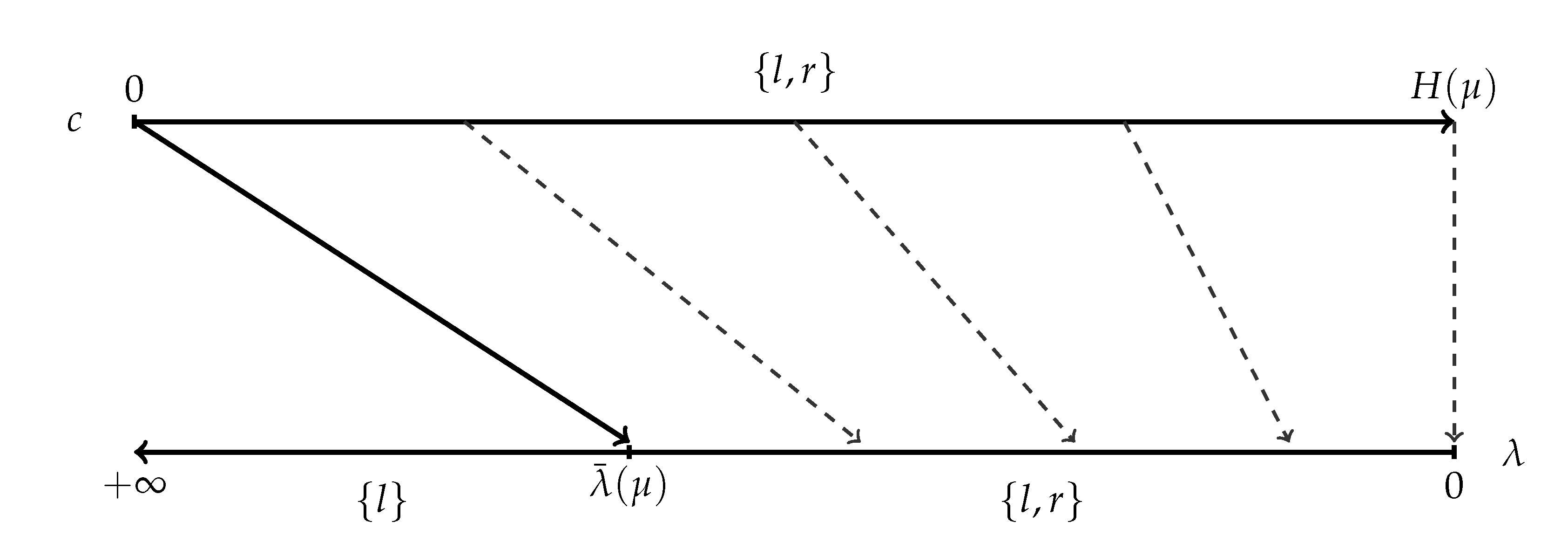
In (*), for , we have , , and determined by . For , the solution is , i.e., no information.
In (**), for any , the consideration set is and . These posteriors are determined by the equation , and the probabilities are then determined by the equation . See Figure 4.
4. Model Comparison
In this section, we state several results regarding the relationship and differences between the two versions of the RI problem. These results generalize the insights that are gained from the above example. All of the proofs not in the main text can be found in the Appendix A.
We start with the following lemma that describes the correspondence between c and . This correspondence is key for the subsequent analysis.
Lemma 1.
Fix a decision problem . For every , there is a unique , denoted , such that every solution to (**) with c solves (*) only with . The mapping is continuous and (weakly) decreasing on , and .
Lemma 1 implies that the choice consistent with optimization in problem (**) with c can be rationalized as optimal behavior in (*) only for one value of , namely . The continuity and monotonicity of imply that its image contains the entire interval . Therefore, for every in this interval, the optimal behavior in (*) can be rationalized as optimal behavior in (**) with some c. However, as illustrated in the example, for a given , there may be multiple solutions that correspond to different values of c, so a solution to (*) with need not be optimal (or even feasible) for (**) with c.
4.1. Consideration Sets and Optimal Posteriors
Perhaps the most apparent difference between the solutions of (*) and (**) in the example is that there is an interval of c values for which the solution of (**) has all three actions considered, while, in (*), this can only happen at a single point , and, even at , there are other solutions that only involve subsets of actions. It is well-known [4] that this feature of the solution of (*) is true in general: in every decision problem, there is always a solution in which the size of the consideration set is, at most, . We now show that, in several cases of interest, the solution of (**) behaves quite differently. Thus, the example of Section 3 is in no way special.
The first result generalizes the example to any decision problem with a binary state-space, at least three actions, and a not-too-extreme prior.
Proposition 2.
Let and denote, by , the (unique) optimal action at . If neither nor are optimal at the prior μ, then there is and , such that, for every (i) and (ii) for every P that solves (**).
In the next proposition, we consider a class of decision problems similar to the one analyzed in (Caplin et al. [9], Section 3.1), but with an additional action corresponding to the outside option of the DM. Let . Consider the decision problem in which , and the utility function is given by
and for every , where . Thus, if the DM correctly guesses the state, then her payoff is 1, while any wrong guess yields a payoff of 0. In addition, the safe choice o guarantees a payoff of t.14 For this class of problems, we obtain a similar result to that of Proposition 2.
Proposition 3.
Consider a decision problem, as described above, and suppose that the prior μ satisfies for every i. Then there is and , such that, for every (i) and (ii) for every P that solves (**).
The assumption that for each i guarantees that the optimal action at the prior is the outside option o, and that is centrally located, in the sense that it is not in the convex-hull of any collection of posteriors at which the actions are optimal.
The intuition for the last two propositions is similar to the one in the example: when is small, the DM obtains precise information guaranteeing that one of the ′extreme′ actions (the ’s) will be selected. When is relatively large, the DM may seek some information, but it will often end up at a posterior in which a safer action is optimal (o in Proposition 3). The transition between these two regimes happens at . Moreover, at , mixtures of these two types of solutions are also optimal, so there is a range of c values mapped to and both types of actions are considered.
Remark 1.
Another known property of (*) is that the same set of posteriors can not be a solution with two different values of λ, while assuming that some information is obtained (this immediately follows from condition (4) above). As shown in the example, this is not true for the parameter c in (**): there is an interval of c values, such that the chosen posteriors are fixed, and only the allocation of mass over these posteriors changes as c varies. The proofs of Propositions 2 and 3 make it clear that the same is also true in these families of decision problems.
An ′Anything Goes′Result
We end this section by arguing that the testable implications of the constrained model are limited if the analyst does not know the DM’s utility function and prior. Namely, any finite set of posteriors that is not convex independent can arise as the solution to problem (**) for an interval of c values in some decision problem. Note that the set of posteriors can be arbitrarily large.
Proposition 4.
Fix Ω, let be an arbitrary integer, and consider a collection of distinct elements in the relative interior of . If Γ is not convex independent (i.e., if there is in the convex-hull of ), then there is a decision problem and such that for every (i) there is a solution of (**), in which the set of posteriors is Γ; and (ii) if , then γ is not part of any solution of (**).
A couple of comments are in order. First, property (ii) of the proposition guarantees that optimal posteriors must be in ; in particular, the decision problem is non-trivial in the sense that not every P is optimal. Second, while we know that the set is also a solution to the unconstrained problem for some , Remark 1 above implies that it is not robustly so in the sense that arbitrarily small changes in would change the optimal set of posteriors. This is in contrast to the constrained version, in which remains optimal for all .
4.2. Comparative Statics
4.2.1. Locally Variant Posteriors
The "locally invariant posteriors" (LIP) property [4] states that changes in the prior do not affect the optimal set of posteriors for (*) whenever this set is still feasible. Dean and Neligh [6] experimentally test this property and find that it is generally satisfied.
In problem (**), on the other hand, arbitrarily small changes in the prior typically induce different sets of optimal posteriors. Consider the example of Section 3 with some given prior , and suppose that c is large enough, so that the optimal consideration set is . The optimal posteriors satisfy in this case. Therefore, by the symmetry of H, the cost of an optimal P is given by . Because the budget constraint binds, we must have . Therefore, if c is fixed and the prior changes, then the optimal posteriors must also change.
The reason for the failure of LIP is clear: suppose that we fix a set of affinely independent posteriors . For in the convex-hull of this set, say , the cost associated with the choice of these posteriors is . The first term is strictly concave in , while the second is linear in (since the vector changes linearly with ). Therefore, with a fixed set of posteriors, the cost is a strictly concave function of the prior , which implies that changes in the prior typically lead to variation in the cost. Because the budget constraint binds, the set of posteriors associated with an optimal solution must adjust to keep the cost unchanged. Therefore, we have the following.
Proposition 5.
Consider a decision problem and parameter c, such that (**) has a unique solution P with posteriors that are affinely independent. Then the set of priors for which the same set of posteriors is optimal for decision problem with parameter c is a nowhere dense subset of .15
Another way to think about the failure of LIP is that, under the conditions of the proposition, for decision problem is usually different than for . When changes, the optimal set of posteriors in (*) changes with it, as mentioned in the previous subsection.
We note that the assumption of affinely independent posteriors can not be dispensed with. Indeed, going back to the example, consider the case and c not too large, so that the solution to (**) has . For close to and the same c, the solution to (**) still has . Additionally, when all three actions are considered, the posteriors must be , , and .
Finally, the difference between the unconstrained and constrained versions of the RI model that are exhibited in Proposition 7 is much more general than in the case where cost is measured by a reduction of entropy. Indeed, both the LIP property in the unconstrained version and its failure in the constrained version continue to hold so long as cost is measured by the expected reduction in the value of a strictly concave function of posteriors.
4.2.2. Utility Scaling
While the solution of problem (**) is sensitive to changes in the prior, it does not change when the stakes of the decision problem are scaled up or down.
Proposition 6.
Consider a decision problem and suppose that P solves (**) with parameter c. Then P is also a solution of (**) with parameter c in the decision problem for every .
The argument is straightforward: since P is optimal in , it follows from Proposition 1 that P solves (*) for this decision problem with some . Therefore, P also solves (*) for the scaled decision problem with . Because the cost of P does not change with the problem, Proposition 1 implies that P also solves (**) for with the same c.
Notice that stakes do matter in the unconstrained version: scaling up the utility has the exact same effect as scaling down the marginal cost of information , which, as already discussed, necessarily changes the solution.
4.3. Optimality of ′No Information′
For large values of , the solution of (*) often involves the DM choosing not to be informed at all, as demonstrated by the example. Indeed, that was the case for any prior , except for . On the other hand, since the budget constraint must bind, choosing no information can not be optimal in (**) for any .
In light of Lemma 1, this gap between the two versions occurs if and only if the limit is finite. Indeed, there is a zero-cost (i.e., uninformative) solution to (*) with if and only if . In the next proposition, we characterize those decision problems for which is finite and show that this is the ′typical′ case.
Formally, we say that P is uninformative if is the same for all , or, equivalently, if the posterior is equal to the prior with probability 1. Additionally, given , say that the prior is an indifference point if there are two different actions , such that both a and are optimal at belief , i.e., . Note that, for a given , the set of indifference points is "small" in , e.g., it is nowhere dense and has Lebesgue measure zero in viewed as a subset of .
Proposition 7.
Suppose that μ is not an indifference point of and let be the (unique) optimal action given belief μ. Then the limit is finite and, for every , the unique solution to (*) is given by for all ω. If μ is an indifference point, then and uninformative P’s are never optimal.
Intuitively, when is large condition (4) that characterizes the solution to (*) requires that the posteriors are close to each other and, therefore, close to the prior . Thus, if is not an indifference point, then, for large enough , the same action that is optimal at is also optimal at all posteriors. But then obtaining no information yields the same expected utility at a lower cost. Conversely, when is an indifference point, the marginal value of little information is positive, since it allows the DM to learn which of the a-priory optimal actions is better. The marginal cost of little information is zero due to the smoothness of the entropy function. Therefore, it is not optimal to obtain no information.
Funding
This research received no external funding.
Institutional Review Board Statement
Not applicable.
Informed Consent Statement
Not applicable.
Conflicts of Interest
The author declares no conflict of interest.
Appendix A. Proofs
Appendix A.1. Notation
The following notation and remarks will be used in several of the proofs below. We use P to denote the state-dependent stochastic choice of the DM, i.e., . The distribution over posteriors induced by P is denoted by . Recall that the support of is the collection , where , and is the probability assigned to posterior . Given and , the mixture of the induced distributions over posteriors is defined as usual: The support of the mixture is the union of the supports of and , and the probability of each in the support is the corresponding average of probabilities of in the two distributions.
Remark A1.
Suppose that P solves either (*) or (**). If , then choosing a must be optimal given belief , that is . Indeed, if that was not the case then choosing the same distribution over posteriors but playing some action from the arg max would increase the utility of the DM without changing the cost of information. Furthermore, a must be the unique optimal action given belief . Indeed, if there are multiple optimal actions at some induced posterior, then this is inconsistent with optimality, as shown in the proof of Proposition 7.
Remark A2.
Given P and , if and the posteriors induced by P and induced by are not equal, then the mixture has two different posteriors associated with the same action a. In particular, if P and are both optimal in (*), and if , then . Indeed, if P and are optimal, then so is any mixture of and .
Given a decision problem , we write
for the expected utility that the DM obtains with choice P. Notice that this can also be expressed using as
Similarly, we write
for the cost of P. Thus, problem (*) can be written as , and problem (**) as subject to .
Appendix A.2. Proofs of Propositions
Proof of Proposition 1.
Fix a decision problem and . We prove here that if P is optimal for (**) then the budget constraint (1) binds. As explained in the text, the rest of the argument is a standard application of the KKT theorem.
For each let . Denote , where . Then a choice P gives the DM expected utility of if and only if for every . Our assumption that different actions are optimal at different states means that whenever . It follows that if P achieves then P reveals the realized state with probability one, and therefore that .
Now, suppose that P is such that the constraint is slack, . Because it follows from the previous paragraph that . For define , where satisfies . Then , and since C is continuous in P we have that for small enough, so is feasible. This shows that P is not a solution for (**). □
Proof of Lemma 1.
Fix c and let P be a solution to (**). By Proposition 1 the budget constraint binds, implying that P must be informative. In particular, there must be two actions such that . Moreover, Proposition 1 implies that there is , such that conditions (4) and (5) are satisfied. From (4) we have that for every
or, after rearranging,
Because we assumed that actions are not duplicates, there exists some at which , which implies that the right-hand side of the last equation is strictly monotone in . It follows that is pinned down uniquely by P. Denote this by .
Now, suppose that also solves (**) with the same c. By Proposition 1 solves (*) with some . We claim that it must be the case that . Indeed since they are both optimal in (**), and, since the budget constraint binds, . This implies that P is also optimal for (*) with , so by the previous paragraph .
Next, we prove that is (weakly) decreasing. Let and suppose per absurdum that . Let P be optimal for (**) with c and optimal for (**) with . Then
where the first inequality follows from P being optimal for (*) with , the next equality holds since the budget constraint in (**) binds, the strict inequality is by the assumptions that and , and the last equality is again by the binding budget constraint. Rearranging gives
contradicting the optimality of for (*) with .
Finally, we show that the image of contains the entire open interval . Combining this with the monotonicity proved above implies both continuity and . Suppose that is in this interval. Let P be optimal for (*) with . Notice that is impossible, since that would imply that any also has an uninformative solution, contradicting the assumption that . It also can not be that since that would require the posteriors to be at the vertices of the simplex, contradicting (4). Thus, and it follows from Proposition 1 that P is also optimal for (**) with . Therefore, , i.e., is in the image. This completes the proof. □
Proof of Proposition 2.
Because there are only two states, we identify distributions over with the probability they assign to . Define to be the set of all , such that there exists a solution P to (*) satisfying . We break the proof into several claims.
Claim 1.
The set is non-empty and bounded from above.
Proof.
If P is optimal and then by (4) we have and also . As we either get and , or vice versa.16 From Remark A1, a and b must be optimal given beliefs and , respectively. This is only possible if when is sufficiently small. It is also clear that choosing ′no information′ is not optimal for small enough, since it is not optimal at . Thus, every sufficiently small is in .
On the other hand, as the ratio converges to 1. Because must be in the convex-hull of the induced posteriors, all the induced posteriors necessarily converge to as (see the proof of Proposition 7 for details). Additionally, since we assumed that neither nor are optimal at , this implies that these actions are not considered for large enough . Thus, is bounded from above. □
Claim 2.
Let . Then in problem (*) with there are two solutions, and , such that and .
Proof.
First, consider a sequence converging to from below, such that for each n there is a solution to (*) with satisfying . Such a sequence exists by the definition of . By taking a subsequence if needed we may assume that converges. By the theorem of the maximum the limit is optimal at . In addition, we must have : For every we have for all n, implying . Additionally, it is impossible that or since these actions are not optimal at .
Second, let be a sequence converging to , but this time from above. Let be a corresponding solution sequence such that for each n.17 Subsequently, the limit is optimal at , and by the definition of we have for every n, also implying that . □
Claim 3.
For and constructed in Claim 2, .
Proof.
Because H is strictly concave over , it is sufficient to show that is a mean-preserving spread of . We consider two different cases. Suppose first that , i.e., neither of the two extreme actions is in the consideration set of . Subsequently, by Remark A1, every posterior induced by is in-between the two posteriors induced by . This implies that is a mean-preserving spread of as needed.
The other case is when . Since has at most two elements, the intersection contains exactly one element, say . Denote the support of by and the support by . Remark A1 implies that . In addition, since both and are optimal, Remark A2 implies that . Therefore, we again get that is a mean-preserving spread of and the claim is proved. If the argument is symmetric. □
So far, we have shown that , and that . By monotonicity proved in Lemma 1 this implies that for every . The next claim completes the proof of the proposition.
Claim 4.
Denote . There is such that if P is optimal for (**) with then .
Proof.
Assume, contrary to the claim, that there is a sequence converging to from below and a corresponding sequence , such that solves (**) with and for every n. Because of the budget constraint binds, we have for all n, so for n large enough also solves (*) with . Denote and the corresponding posteriors by (it can not be that since then ). Additionally, recall that are the posteriors induced by . There are three cases to consider:
First, it can not be that , since by Remark A2 this would imply and , contradicting the assumption that .
Second, suppose that for some action . Then again by Remark A2 this would imply . Additionally by Remark A1 the other posterior is smaller and bounded away from , contradicting the assumption that . The argument for is analogous.
Third, if , then both and are between and bounded away from , so can not converge to . □
Proof of Proposition 3.
For the most part the proof follows the footsteps of the proof of Proposition 2. We only provide details when a different argument is needed.
Claim 5.
For any , if P solves (*) then either or .
Proof.
Suppose by contradiction that P is optimal and . From Remark A1, if then the associated posterior must satisfy , implying that for any . Let i be such that . Then
contradicting the assumption in the proposition. □
Define to be the set of all , such that there exists a solution P to (*), satisfying .
Claim 6.
The setis non-empty and bounded from above.
Proof.
We first prove that, if is small enough and P solves (*), then . By Claim 5, this implies that , so .
Summing up over all i gives
Since this inequality clearly can not hold for small enough.
To show that is bounded, note that the assumption of the proposition implies that o is the unique optimal action at . By Proposition 7, this implies that obtaining no information is the unique optimal choice for all large enough. □
Claim 7.
Let . Then in problem (*) with there are two solutions, and , such that and .
Proof.
The proof is identical to that in Claim 2, except that to argue that we need to use Claim 5. □
Claim 8.
For and constructed in the previous claim, .
Proof.
We denote by the posterior corresponding to induced by and by the one induced by (if ).
Because , must coincide with the solution given in ([9], Theorem 1) when all of the ’s are considered. In particular, the induced posteriors are symmetric in the sense that is the same for all i. It follows that . On the other hand, by Remark A2 we must have whenever , implying that
where the strict inequality follows from (recall Claim 5) and . Therefore, we got that , and since both are optimal for (*) with it must be that . □
Claim 9.
Denote . There is such that if P is optimal for (**) with then .
Proof.
Suppose by contradiction that , and that for each n solves (**) with but . Then , so for n large enough also solves (*) with . Since we can not have , so by Claim 5 . The exact same argument as in the previous claim gives . Moreover, is bounded away from zero, since is not in the convex-hull of any strict subset of . This implies that there is such that for every n. However, and are both optimal for (*) with , so . This contradicts the convergence of to . □
Proof of Proposition 4.
Fix a collection as in the proposition. Define by . Because f is strictly convex, for each there is an affine function such that and for every . Let the set of actions be and the utility function be , where is the Dirac measure on state .
To complete the description of the decision problem we need to choose the prior . By assumption, one of the elements of , say , is in the convex hull of the others. Define for some .
Consider the set
We claim that this set contains a non-degenerate interval of c values. Indeed, one element of this set is . Additionally, we have for some probability vector , so is also in this set. The strict concavity of H implies that the former is strictly larger than the latter. By taking convex combinations of these two representations of we can get any c in between. Denote and . Note that .
Finally, consider problem (**) with . Subsequently, by the definition of and , there are strictly positive satisfying and . We claim that this distribution over posteriors is optimal. Indeed, this gives an expected utility of
where the first equality is by the definition of u and the affinity of , the inequality is obvious, the next equality follows from , and the last equality is by construction of . On the other hand, for any feasible distribution over posteriors we have
where the first equality is again by the definition of u and the affinity of , the inequality follows from for all j, and the last inequality follows from feasibility (the reduction of entropy must be at most c). Moreover, if for some i, then for every j, so the first inequality is strict. This completes the proof. □
Proof of Proposition 7.
From Proposition 1 and Lemma 1 it immediately follows that is equal to the infimum of the set of ’s for which an uninformative P is optimal in problem (*). Thus, to prove the proposition, it is enough to show that is an indifference point if and only if the set of such ’s is empty.
We start by showing that if is not an indifference point then for large enough the optimal solution to (*) is uninformative. For this proof, we view as the unit simplex of endowed with the metric . Let
be the set of beliefs at which is the unique optimal action. Because K is relatively open in and , there is such that whenever .
Let . Suppose that is large enough, so that . If P is optimal for (*) with , the, n for every and every , we have
where the first equality is by (4), and the next inequality is by the definition of M. We thus get
where in the first equality we used the fact that optimal posteriors are never on the boundary of (implied by condition (4)), and the following inequality is by (A1).
Now, since , we also have for every and every
Taking the maximum over gives
where the last inequality is from (A2). By the construction of this implies that for every . Thus, by Remark A1, P induces a unique posterior and is therefore uninformative.
In the other direction, we now claim that, if is an indifference point, then an uninformative P can not be a solution of (*) with any . Indeed, let be two optimal actions given belief . Consider , as given by for every . Note that is optimal among the set of uninformative P’s. However, we have and . Because are not duplicates, condition (4) can not hold for any , implying that is not optimal.18 □
Appendix A.3. Proofs of Claims in the Example
We start with the following lemma.
Lemma A1.
- (i)
- For : .
- (ii)
- For : and .
- (iii)
- For : , and .
Proof
- (i)
- Condition (4) with and requiresin state andin . It is immediate to verify that these two equations are equivalent to .
- (ii)
- Similarly, condition (4) with and requiresin andin , and these two equations are satisfied if and only if the posteriors are as in the lemma.
- (iii)
- When all three actions are considered condition (4) is equivalent to the equations in both previous cases holding simultaneously. In particular, it implies that both and . This pins down at , and consequentially the posteriors , as above.
□
Case 1:
Claim 10.
Solution of (*): If then and . If then and . If then any mixture (including degenerate) of the former two solutions is optimal.
Proof.
Suppose , and we will show that is optimal. From Lemma A1 (i), condition (4) is equivalent to . Condition (5) with and requires
Plugging in and rearranging, this condition becomes , which holds by assumption. Condition (7), with and , is identical, given that .
Suppose now that . We need to show that obtaining no information is optimal. Condition (4) is trivially satisfied, so we only need to check (5) for and . For , this gives
which is equivalent to . For , we get the exact same condition.
Finally, when it follows from the last two paragraphs that both and are still optimal. Because the set of optimal distributions over posteriors is convex, it follows that any mixture of these solutions is optimal as well. Note that at the posteriors of the risky actions in the solution are given by . □
Claim 11.
Solution of (**): If then the solution is given by , , , and . If then and is determined by the equation .
Proof.
Suppose . We show that is optimal. From Lemma A1 (iii) it must be that , , and that the value of the lagrange multiplier is . Setting and , we get that . In addition, the expected reduction of entropy from the prior to the posteriors is given by
so the budget constraint (6) binds. By Proposition 1, we are done.
Once it is no longer possible that all three actions are considered, since, given the location of the posteriors, the budget constraint can not bind. We show that is optimal. Define by the equation , and set . Let . Subsequently, and the budget constraint binds. Set to solve . Afterwards, condition (4) is satisfied by Lemma A1 (i). Furthermore, since we know that , which implies that . Thus, (5) holds for and in the same way as in the case of the previous claim. □
Case 2:
Claim 12.
Solution of (*): When we have , , and the probabilities are set to satisfy . At the solution is not unique, with , , and all possible. When , , the posteriors are , , and the probabilities are adjusted, so that . Finally, for , it is optimal to obtain no information, and the consideration set is either or when is below or above , respectively.
Proof.
The proof for is identical to the case. Suppose that and we prove that is optimal. By Lemma A1 (ii), condition (4) is equivalent to and . We need to check condition (5) with and . For , this requires
which boils down to . For , the condition is
which, again, is equivalent to . Finally, we need that is in the interior of the convex hull of and . It is not hard to check that this is equivalent to .
Note that at both solutions with and with are optimal, and therefore any mixture is optimal as well. This implies that is also optimal.
Suppose now that . We consider the case where , so obtaining no information implies that and (the case in which is similar). We need to check (5) with and . These conditions are given by
and
respectively. For every , the second inequality implies the first, and it is satisfied if and only if . This completes the proof. □
Claim 13.
Solution of (**): For the consideration set is , and the distribution over posteriors is determined by the equations , and . For the consideration set is , the posteriors are , and the probabilities adjust so that the expected posterior is equal to and the cost is equal to c. For , the consideration set is , the posteriors are determined by and , and their probabilities by .
Proof.
Fix c in the first range. The function is strictly increasing on , strictly decreasing on , and is equal to at both and . It follows that, for each , there is a unique , such that , and that as increases the corresponding decreases. Therefore, given , there is a unique way to choose the posteriors and the probabilities , such that (1) ; (2) ; and, (3) .19 Now, define as the (unique) solution to , and note that this implies . By Lemma A1 (ii) condition (4) holds. Finally, implies that , so condition (4) holds in the same way as in the previous claim.
Moving on to , the distribution in the claim is optimal by Proposition 1 with . The lower end of the range of c is obtained by the distribution with support and only, while the upper end by the distribution with support and only.
When the proof is as in the previous claims. □
Case 3:
Claim 14.
The solution of (*): for we have , , and determined by . For , the solution is , i.e., no information.
Proof.
Fix and set the posteriors as in the claim. Subsequently, (4) holds by Lemma A1 (i). As in the previous cases above, condition (5) with and is equivalent to ; for in the current range it is easy to check that , so the condition holds by assumption. Finally, we need that , which is equivalent to .
Assume now . Set and . Condition (5) with and requires
and
respectively. For any in the range, the second inequality implies the first and it is satisfied if and only if . □
Claim 15.
The solution of (**): For any the consideration set is and . The posterior is determined by the equation , and the probability is then determined by the equation .
Proof.
Fix c and define by . Let and set to solve . The fact that implies that , which in turn implies that as well as that . The optimality of these posteriors now follows in the same way as in the previous claim. □
References
- Sims, C.A. Stickiness. Carnegie Rochester Conf. Ser. Public Policy 1998, 49, 317–356. [Google Scholar] [CrossRef]
- Sims, C.A. Implications of rational inattention. J. Monet. Econ. 2003, 50, 665–690. [Google Scholar] [CrossRef] [Green Version]
- Shannon, C.E. A mathematical theory of communication. Bell Syst. Tech. J. 1948, 27, 379–423. [Google Scholar] [CrossRef] [Green Version]
- Caplin, A.; Dean, M. Behavioral Implications of Rational Inattention with Shannon Entropy; National Bureau of Economic Research: Cambridge, MA, USA, 2013. [Google Scholar]
- Le Treust, M.; Tomala, T. Persuasion with limited communication capacity. J. Econ. Theory 2019, 184, 104940. [Google Scholar] [CrossRef] [Green Version]
- Dean, M.; Neligh, N. Experimental Tests of Rational Inattention. Working Paper. 2019. Available online: http://www.columbia.edu/~md3405/Working_Paper_21.pdf (accessed on 29 December 2020).
- Maćkowiak, B.; Matějka, F.; Wiederholt, M. Rational Inattention: A Review. Working Paper. 2020. Available online: http://home.cerge-ei.cz/matejka/RIsurvey.pdf (accessed on 29 December 2020).
- Matějka, F.; McKay, A. Rational inattention to discrete choices: A new foundation for the multinomial logit model. Am. Econ. Rev. 2015, 105, 272–298. [Google Scholar] [CrossRef] [Green Version]
- Caplin, A.; Dean, M.; Leahy, J. Rational inattention, optimal consideration sets, and stochastic choice. Rev. Econ. Stud. 2019, 86, 1061–1094. [Google Scholar] [CrossRef] [Green Version]
- Caplin, A.; Dean, M.; Leahy, J. Rationally Inattentive Behavior: Characterizing and Generalizing Shannon Entropy; National Bureau of Economic Research: Cambridge, MA, USA, 2017. [Google Scholar]
- Matějka, F. Rigid pricing and rationally inattentive consumer. J. Econ. Theory 2015, 158, 656–678. [Google Scholar] [CrossRef] [Green Version]
- Steiner, J.; Stewart, C.; Matějka, F. Rational inattention dynamics: Inertia and delay in decision-making. Econometrica 2017, 85, 521–553. [Google Scholar] [CrossRef]
- De Oliveira, H. Axiomatic Foundations for Entropic Costs of Attention. Working Paper. 2014. Available online: https://6964c30c-a4a4-4464-a435-9021be4b7ccd.filesusr.com/ugd/21e9a6_dab3d6bc526d40fa86894de99e3a48ba.pdf (accessed on 29 December 2020).
- Fulton, C. Mechanics of Linear Quadratic Gaussian Rational Inattention Tracking Problems. Working Paper. 2017. Available online: https://papers.ssrn.com/sol3/papers.cfm?abstract_id=3065488# (accessed on 29 December 2020).
- Doval, L.; Skreta, V. Constrained Information Design: Toolkit. Working Paper. 2018. Available online: https://arxiv.org/abs/1811.03588 (accessed on 29 December 2020).
- Boleslavsky, R.; Kim, K. Bayesian Persuasion and Moral Hazard. Working Paper. 2020. Available online: https://papers.ssrn.com/sol3/papers.cfm?abstract_id=2913669 (accessed on 29 December 2020).
- Caplin, A.; Dean, M. Revealed preference, rational inattention, and costly information acquisition. Am. Econ. Rev. 2015, 105, 2183–2203. [Google Scholar] [CrossRef] [Green Version]
- Dewan, A.; Neligh, N. Estimating information cost functions in models of rational inattention. J. Econ. Theory 2020, 187, 105011. [Google Scholar] [CrossRef]
- Cheremukhin, A.; Popova, A.; Tutino, A. A theory of discrete choice with information costs. J. Econ. Behav. Organ. 2015, 113, 34–50. [Google Scholar] [CrossRef]
- Rockafellar, R.T. Convex Analysis; Princeton University Press: Princeton, NJ, USA, 1970. [Google Scholar]
| 1. | The use of entropy for measuring quantity of information has its origins in [3] classical work on the capacity of a communication channel. |
| 2. | More precisely, the agent chooses both the information structure and the action to take conditional on the realized signal. See the next section. |
| 3. | The Lagrangian contains additional terms due to constraints associated with x being a collection of probability distributions. These constraints are common to the two versions and are not relevant for the current discussion. |
| 4. | Le Treust and Tomala [5] give an example that is similar to ours, where the number of actions considered is larger than the number of states in the constrained problem. They prove that there is always a solution with at most the number of states plus one actions. We discuss the relation to that paper below. The first draft of the current paper was written without awareness of this existing result. |
| 5. | See the related literature section below for a discussion of experimental works that test some of these implications. |
| 6. | |
| 7. | |
| 8. | Dewan and Neligh [18] also compare the performance of several cost functions for information in explaining their data. They find that most of the subjects fit well to one of four functional forms, including Shannon entropy; however, they do not explicitly consider the constrained model. |
| 9. | If , then full information is feasible and the problem becomes trivial, similarly to the case in (*). |
| 10. | Indeed, starting from , define and let for any . In the other direction, set . |
| 11. | Because the setup is symmetric the analysis is similar for . |
| 12. | Note that, for , we have , so the latter case is empty. |
| 13. | This happens when . |
| 14. | In Caplin et al. [9], the available actions are just . Setting the payoffs to 1 and 0 is just for convenience, the same result (with the obvious changes) applies with similar payoff structures. |
| 15. | We view as a subset of the Euclidean space and endow it with the topology that it inherits from that space. A set in a topological space is nowhere dense if its closure has an empty interior. The proposition immediately follows from the fact that the level sets of a strictly concave and continuous function are closed and contain no open set. |
| 16. | If one of the actions (weakly) dominates the other then the latter can not be part of an optimal solution. |
| 17. | Recall that there is always a solution in which the size of the consideration set is at most the number of states [4]. |
| 18. | The same argument also implies the stronger result that if P is optimal for (*) with some , then none of the posteriors is an indifference point. |
| 19. | Note that the bound on c is obtained by setting and . |
Figure 1.
The dashed lines show the expected utility for each of the actions in the example as a function of the decision maker’s (DM’s) belief. The upper envelope of these functions is the solid black line. l is optimal for posteriors in , m is optimal in , and r is optimal in .
Figure 1.
The dashed lines show the expected utility for each of the actions in the example as a function of the decision maker’s (DM’s) belief. The upper envelope of these functions is the solid black line. l is optimal for posteriors in , m is optimal in , and r is optimal in .
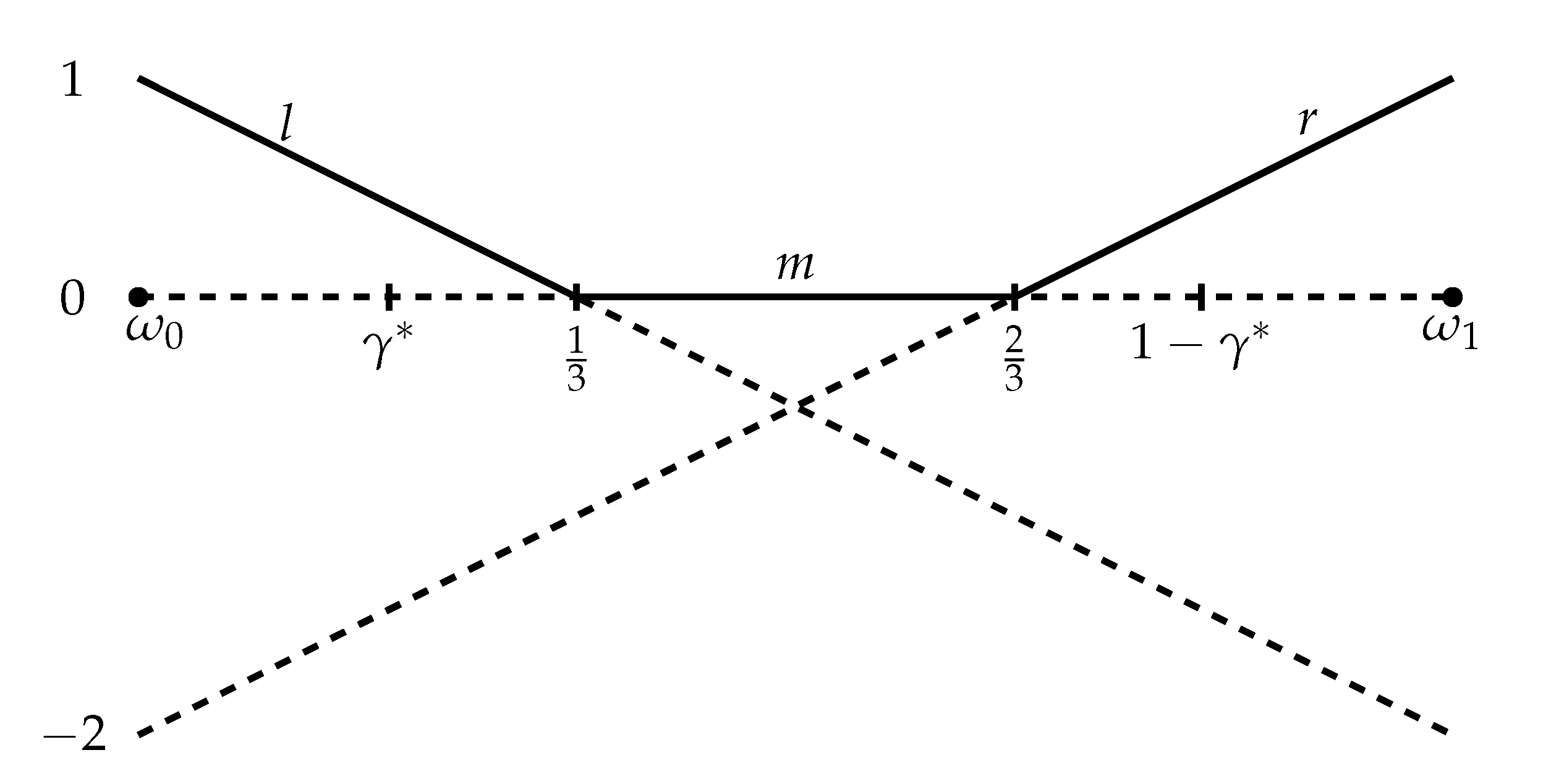
Figure 2.
The solutions of problems (**) (upper line) and (*) (lower line) from the example with prior . The arrows between the lines illustrate the mapping from c to the value of the lagrange multiplier at the optimum.
Figure 2.
The solutions of problems (**) (upper line) and (*) (lower line) from the example with prior . The arrows between the lines illustrate the mapping from c to the value of the lagrange multiplier at the optimum.
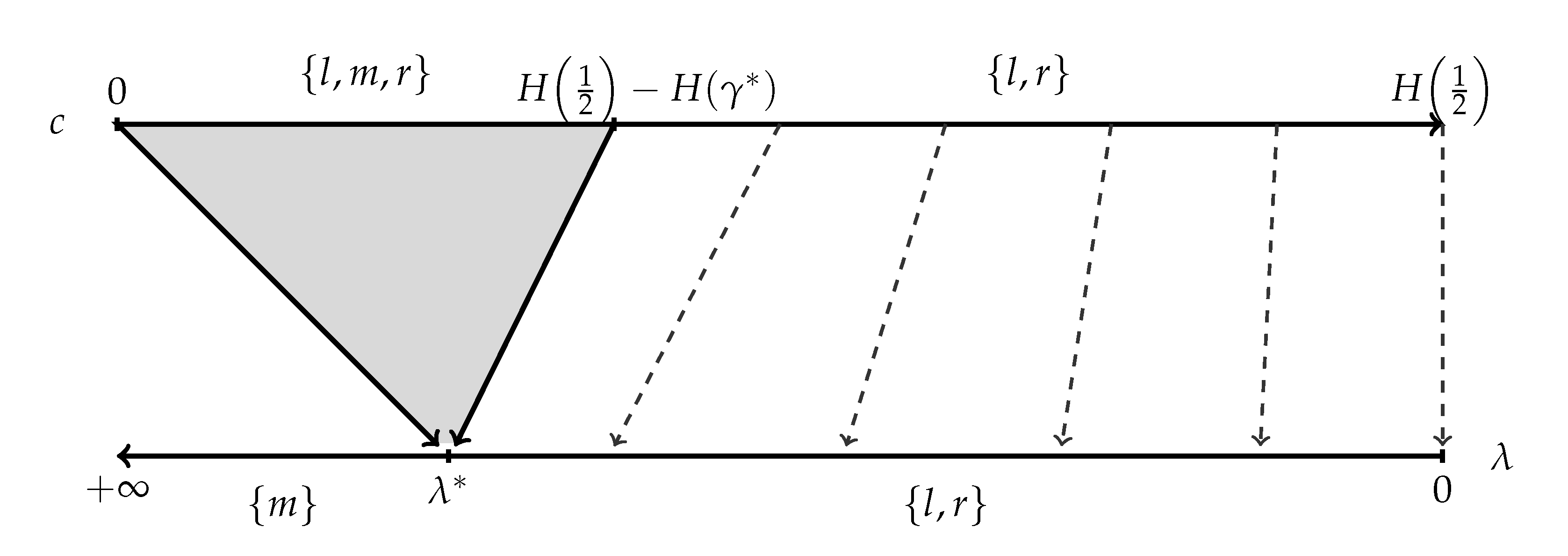
Figure 3.
The consideration sets in the solutions of (*) and (**) for the case , . When , the consideration set in (*) is for every .
Figure 3.
The consideration sets in the solutions of (*) and (**) for the case , . When , the consideration set in (*) is for every .
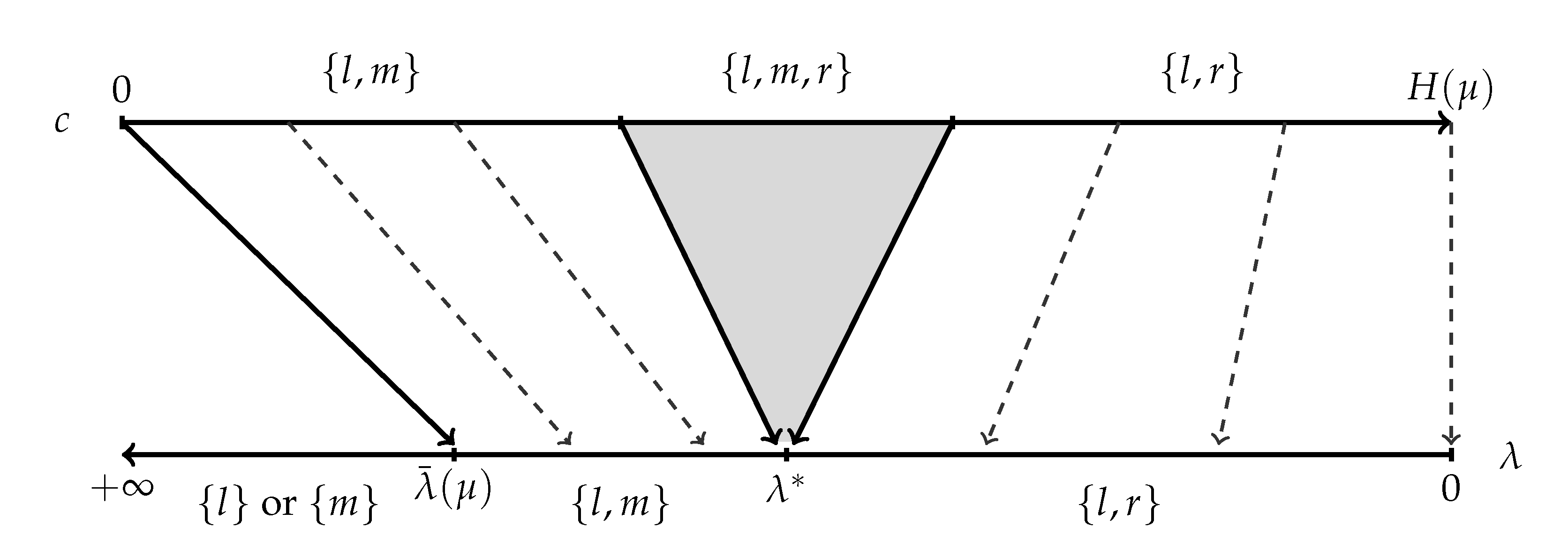
Figure 4.
The solution of the example for .
Publisher’s Note: MDPI stays neutral with regard to jurisdictional claims in published maps and institutional affiliations. |
© 2021 by the author. Licensee MDPI, Basel, Switzerland. This article is an open access article distributed under the terms and conditions of the Creative Commons Attribution (CC BY) license (http://creativecommons.org/licenses/by/4.0/).
Share and Cite
MDPI and ACS Style
Azrieli, Y. Constrained versus Unconstrained Rational Inattention. Games 2021, 12, 3. https://0-doi-org.brum.beds.ac.uk/10.3390/g12010003
AMA Style
Azrieli Y. Constrained versus Unconstrained Rational Inattention. Games. 2021; 12(1):3. https://0-doi-org.brum.beds.ac.uk/10.3390/g12010003
Chicago/Turabian StyleAzrieli, Yaron. 2021. "Constrained versus Unconstrained Rational Inattention" Games 12, no. 1: 3. https://0-doi-org.brum.beds.ac.uk/10.3390/g12010003
Note that from the first issue of 2016, this journal uses article numbers instead of page numbers. See further details here.