
A Model of Protocoalition Bargaining with Breakdown Probability

School of Economics, University of Nottingham, University Park, NG7 2RD Nottingham, UK
Games 2015, 6(2), 39-56; https://0-doi-org.brum.beds.ac.uk/10.3390/g6020039
Submission received: 1 January 2015
/
Revised: 16 March 2015
/
Accepted: 23 March 2015
/
Published: 22 April 2015
(This article belongs to the Special Issue Political Economy and Game Theory)
Abstract
:This paper analyses a model of legislative bargaining in which parties form tentative coalitions (protocoalitions) before deciding on the allocation of a resource. Protocoalitions may fail to reach an agreement, in which case they may be dissolved (breakdown) and a new protocoalition may form. We show that agreement is immediate in equilibrium, and the proposer advantage disappears as the breakdown probability goes to zero. We then turn to the special case of apex games and explore the consequences of varying the probabilities that govern the selection of formateurs and proposers. Letting the breakdown probability go to zero, most of the probabilities considered lead to the same ex post pay-off division. Ex ante expected pay-offs may follow a counterintuitive pattern: as the bargaining power of weak players within a protocoalition increases, the weak players may expect a lower pay-off ex ante.
JEL classifications:
C78; D721. Introduction
The Baron-Ferejohn [1] model is the most frequently used formal model of legislative bargaining. In this model, there are n identical legislators, and decisions are made by simple majority. An agent is selected at random (each agent with probability ) to propose a division of the budget. If a majority votes in favour of the proposal, the proposal is implemented, and the game ends (closed rule); otherwise, a new proposer is selected at random, and the process continues until an agreement is reached.1
Even though coalitions are not explicitly formed in this model, we can think of the set of players who vote yes as the coalition that forms. Given this interpretation of the model, players are able to agree simultaneously on coalition formation and pay-off division.2 However, in the context of government formation, it is natural to think of parties as forming tentative coalitions (protocoalitions)3 before beginning negotiations over pay-off division. Alternatively, in the context of party formation, legislators may coalesce into a majority party and subsequently decide on what policy to enforce.4
There have been several models of legislative bargaining with protocoalitions in the literature. In Baron and Diermeier [9], once the protocoalition is agreed upon, the formateur makes a take-it-or-leave-it offer; if this offer is rejected, an exogenously-specified status quo prevails. In Diermeier et al. [10], bargaining continues indefinitely between the members of the protocoalition. Breitmoser [11] allows the formateur to revise the chosen protocoalition after a rejection and also allows players to pre-commit to accepting or rejecting certain proposals; the identity of the formateur remains constant throughout.
The present paper analyses a variant of the Baron-Ferejohn model with protocoalition bargaining. Proposers are randomly selected both at the protocoalition formation stage and at the pay-off division stage. The distinctive feature of this model is that negotiations over pay-off division may break down, in which case the protocoalition is dissolved and the process starts again from the beginning, i.e., a formateur is selected anew. This property makes the process stationary and easier to analyse, but it also makes the breakdown outcome endogenous.5
We show that all stationary subgame perfect equilibria of this model have immediate agreement. The value of the breakdown probability does not affect the nature of the equilibrium, but it does affect the proposer advantage within a protocoalition; this proposer advantage vanishes as the breakdown probability goes to zero.
We then turn to some particular classes of games, assuming that symmetric players have the same probability of being selected as formateurs and also the same probability of being selected as proposers within a protocoalition. Under these assumptions, games in which all players are symmetric are straightforward to solve. Only minimal winning coalitions form, and ex post pay-off division varies with the probability that the protocoalition breaks down. If the protocoalition breaks down with certainty after a proposal is rejected, we are essentially back in the original Baron-Ferejohn model; if the breakdown probability tends to zero, pay-off division within the coalition converges to the equal division.
The next case we consider is that of apex games. Apex games are games with one major player and minor players. A minimal winning coalition can be formed by the apex player and any one of the minor players or by all minor players together. Apex games are one of the simplest instances of majority games in which not all players are symmetric6; they are also empirically common7. We explore the consequences of varying the probabilities governing the selection of proposers and formateurs8. It turns out that there is a large parameter region with the property that the equilibrium is competitive in the sense that all players are indifferent between proposing any of the minimal winning coalitions to which they belong. Namely, conditional on the minor player protocoalition forming, each minor player expects ; conditional on the protocoalition of one minor player and the apex player forming, the apex player expects and the minor player expects . These are conditional expected pay-offs; if moreover, we take the limit as the breakdown probability goes to zero, ex post pay-off division also converges tothese values.
Even though expected pay-offs conditional on a particular protocoalition forming are quite robust to changes in the formateur and proposer probabilities, ex ante expected pay-offs are affected both directly and indirectly (i.e., through changes in equilibrium strategies) by these probabilities. It turns out that this effect does not always go in the intuitive direction. If we increase the bargaining power of a player within a protocoalition, equilibrium strategies may adjust in such a way that this player is less likely to be included in the protocoalition that forms and may actually be worse-off as a result.
2. The Model
Let be the set of players (parties). There is a budget of size one to be divided and for all i, and is the set of all possible allocations. Player i’s preferences are described by the utility function . The voting rule is described by the set W of winning coalitions, where a winning coalition is a coalition that can enforce any alternative in X. We assume that W is such that, if S is winning, is not winning. Furthermore, if , then for all . We also assume that there are no veto players, that is no player belongs to all winning coalitions. A coalition S is called minimal winning if S is winning and no is winning.
Bargaining proceeds as follows: Nature selects a formateur according to a probability distribution9 ( for all i and ). The selected formateur i proposes a protocoalition with . Players in S accept or reject the proposal sequentially10. If all players in S accept, protocoalition S is formed. If one of them rejects, Nature selects a new formateur according to the probability distribution θ.
Once protocoalition S is formed, players in S bargain over the division of the budget. The “internal” game, played only by players in S, proceeds as follows. A player in S is selected to be the proposer according to a probability distribution with for all and .11 A proposal is a division of the budget between the players in S ( for all and ). As in other papers on protocoalition bargaining, agreement within S on pay-off division needs to be unanimous. If all responders in S (moving sequentially) accept the proposal, the game ends with pay-off vector for players in S (players in get zero). If one of the responders rejects the proposal, two things may happen. With probability p (), bargaining within S continues and a new proposer is selected according to ; with probability , coalition S is dissolved. If coalition S is dissolved, Nature selects a formateur again according to the probability distribution θ.
We denote the non-cooperative bargaining game described above as , or simply G. We will be interested in stationary subgame perfect equilibria (SSPE).
We will refer to the probability distribution θ as the protocol and to as the internal protocol. Given an SSPE , we will denote by y the expected equilibrium pay-off vector computed before Nature starts the game and by the expected equilibrium pay-off vector computed after S has formed and before Nature selects a proposer. Let be the vector of continuation values (i.e., expected pay-offs after a proposal has been rejected) in the internal game. Notice that because of stationarity, y, and depend on , but not on history. We start by computing the equilibrium of the internal game.
2.1. The Equilibrium of the Internal Game
Suppose we have an SSPE of the game with associated expected equilibrium pay-off vector y. We now show that, for any , the internal game has a unique stationary subgame perfect equilibrium pay-off vector , and this pay-off vector is related to y by a simple formula.
Lemma 1. Let be an SSPE of the game G with associated expected pay-off vector y. For any , expected equilibrium pay-offs in the subgame starting right after players agree to form S are given by:
Agreement is immediate if .
Proof. By stationarity, continuation values after S has formed and a proposal has been rejected do not depend on history and can be found in the following way. With probability p, bargaining continues within S (so that player i expects to get ); and with probability , coalition S breaks apart, and the process continues from scratch (so that player i expects to get ). We have the following equation for the continuation value of player i:
Note that, if we add up the above equation over , we obtain . If , it follows that , and the arguments in Okada [17] can be adapted to show that the equilibrium must exhibit immediate agreement.
As a responder, player i must accept any offer strictly above . As a proposer, if player i offers each for a sufficiently small ϵ, this would be more than , so player i strictly prefers to make a proposal that will be immediately accepted rather than one that would be rejected, and agreement occurs in the first round. Each responder must be offered exactly in equilibrium (otherwise, the proposer could cut the responder’s pay-off).
Taking this into account, if , is given by the probability that i is selected to be a proposer in the internal game times his expected pay-off as a proposer plus the probability that he is selected to be the responder (which is because agreement must be unanimous in the internal game) times his continuation value.
If agreement does not occur immediately, the equations above are still valid. Because can be at most one, we have , that is player i may strictly prefer to make a proposal that will be accepted or may be indifferent, but never strictly prefers to create delay by making an unacceptable proposal. The equality occurs when , which, in turn, requires and In this case, we can write the proposer pay-off as irrespective of whether the proposal is accepted or not; likewise, the equilibrium pay-off as a responder is irrespective of whether the proposal is accepted or rejected. All players in S would be indifferent between agreeing and not agreeing.
From this system of equations (and taking into account that ), we see that:
☐
This is a well-known result in bargaining games with breakdown probability: player i’s expected pay-off equals the breakdown pay-off (in this case, ) plus a share of the surplus proportional to the probability of being the proposer (cf. Binmore [18] and Binmore et al. [19]). Note that in this case, the breakdown outcome is endogenous, as in Rubinstein and Wolinsky [20].
Lemma 1 applies to any protocoalition S, including those that are never formed on the equilibrium path.
Except for some degenerate cases (such as , in which players would be indifferent between agreeing and disagreeing), agreement within the protocoalition occurs immediately.
The proposer’s advantage is the difference between the pay-off a player would get as a proposer and the pay-off the same player would get as a responder. The proposer’s advantage is a decreasing function of p. As , the proposer advantage vanishes. As in [19], the possibility of breakdown provides an incentive for the players to reach an agreement. It reduces a player’s continuation value, since, if a proposal is rejected and breakdown occurs, the player will have to start over the bargaining process with the set of players N rather than continue with the smaller set S. The proposer can then offer a lower pay-off to the responders and benefits as a result. As the breakdown probability goes to zero, responders have less to lose by rejecting a proposal, and the proposer advantage vanishes.
Lemma 2. The proposer’s advantage is decreasing in the continuation probability p and vanishesas .
Proof. Player i gets as a proposer and as a responder. Using (1), we have . Since regardless of whether agreement occurs immediately, the proposer advantage equals . ☐
Note that p only affects the results through the proposer advantage. The average pay-offs conditional on S forming, , are unaffected by p.
2.2. The Equilibrium of the Game
Under relatively weak conditions, agreement is reached immediately (cf. [17]).
Proposition 3. If for all i, for all winning coalitions and there are no veto players, then in any SSPE of G, all proposals are accepted, and a protocoalition forms immediately.
Proof. The rules of the game ensure that . A proposal to form a protocoalition S with is always accepted, because the expected pay-off from accepting the proposal, , is strictly greater than the expected pay-off from rejecting it, , for all .12 Consider the situation of i as the formateur. There is always a coalition that i can propose with . This is because is winning for all j; thus, player i can propose any where j is such that . The only case in which this would not be possible is if , but clearly, this cannot happen in equilibrium, because all other players would propose coalitions without i (and such coalitions would be accepted), resulting in i getting zero with a positive probability, contradicting .
On the equilibrium path, i proposes a winning coalition S with , and bargaining between players in S results in immediate agreement. ☐
Corollary 4. If in addition for all i, then in any SSPE of G, we have for all i.
Proof. This is because there is a coalition with , and a proposal by i to form S would be accepted. Since , player i expects a positive pay-off when S is formed. ☐
Two conditions must be satisfied in a no-delay equilibrium: first, the proposer must behave optimally in the sense of only proposing the most profitable coalitions given the vector of expected equilibrium pay-offs y; second, expected equilibrium pay-offs must be consistent with the strategies played. We state these two conditions as Corollaries 5 and 6. These corollaries will be useful in the construction of the equilibria in Section 4.
Corollary 5. The formateur will propose a protocoalition S that solves the following problem:
Because the solution of this problem is sure to have , the formateur does not need to worry about acceptance.
Corollary 6. Let be the probability that player i proposes coalition S. Under the conditions of Proposition 3, the following must hold in any SSPE of G:
The expected equilibrium pay-off has two parts. With probability , player i is chosen to be the formateur. As formateur, player i proposes protocoalition S with probability ; this proposal is accepted, since we are in a no-delay equilibrium by Proposition 3, and player i expects . The second part of the pay-off refers to the case in which a player other than player i is chosen as the formateur; player j is selected with probability and will propose each coalition with probability . Since all proposals are accepted, when a protocoalition is proposed, player i expects a pay-off equal to .
3. Symmetric Games
Consider the case where N consists of n symmetric players and is the number of votes needed for a coalition to be winning. If we further impose symmetry of the protocol (i.e., and for all i and S) and of the equilibrium strategies, we have and for all . Clearly, only protocoalitions of size q will form. The pay-off is just an average conditional on protocoalition S forming; realized pay-off division depends on the breakdown probability p.
Suppose a protocoalition S of size q has been formed and a proposal to divide the pay-off has been rejected. The continuation value for any of the members of S is calculated as follows: with probability p, bargaining continues and player i expects ; with probability , breakdown occurs and Nature restarts the game from the beginning, in which case i expects . Thus:
For , the continuation value is , and we are effectively back in the original Baron-Ferejohn model with a substantial proposer advantage. For , the proposer advantage vanishes and approaches .
For example, if and , yields the original model in which the coalition partner receives and the proposer receives . If , we have , and the proposer receives . In the limit when , each of the two members of the coalition receives .
4. Apex Games
Let . Let Player 1 be the apex player. In an apex game, the set of minimal winning coalitions contains only two types of coalitions: all coalitions of the form , where , and coalition (the minor player coalition). We will consider only protocols that treat all minor players equally, that is for any i, , for any two minor players i and j such that , and for any with , and . For simplicity, we focus on equilibrium strategies with the property that all minor players follow the same strategy and are treated symmetrically by the apex player strategy. We refer to such strategies as symmetric strategies.13
Since all minor players are treated symmetrically, we will use the index m to denote an arbitrary minor player and to denote the coalition of the apex player and a minor player.
If we make no further assumptions on θ and , proposed coalitions are not necessarily minimal winning.
Suppose for some . Then, player i is facing a trade-off: i receives a higher share of the surplus in T, but the surplus of T is smaller. Example 7 shows that the first effect may predominate. This is not completely obvious, because is endogenous.
Example 7. Consider the apex game with seven players . Suppose , , and , where s is the number of players in 14 There is an equilibrium in which the apex player forms a coalition with two minor players.
Let the apex player propose to two minor players at random; thus, each minor player has a probability of receiving a proposal if the apex player is selected to be the formateur. Let the minor players propose coalition . Given these strategies, the equilibrium pay-offs can be found from thefollowing equations:
The solution is , . Player 1 is behaving optimally, because is maximized for . The minor players are also behaving optimally by proposing coalition . In , they expect a pay-off of . If instead, they proposed , they would get a pay-off of .
If we make the additional assumption that , for all and for all , adding extra players to the protocoalition can only reduce the available surplus (indeed, since for all i by Corollary 4, it strictly reduces it). Hence, only protocoalitions in which all responders are pivotal will be proposed in equilibrium. For apex games, this is equivalent to saying that only minimal winning coalitions will be proposed.
Recall that we consider only protocols that treat minor players symmetrically, that is for all , for all and for all , with α and . As for coalitions larger than minimal winning, it is enough to assume for all , so that they will not be optimal.
Proposition 8. Consider the game , where W is an apex game and θ and satisfy the assumptions above. Then:
- (1)
- If , minor players propose coalition in the unique symmetric SSPE. Expected equilibrium pay-offs for the apex player, , are increasing in and α within this region.
- (2)
- If , minor players randomize between proposing coalition and proposing coalition . Expected pay-offs conditional on a protocoalition being formed equal and , irrespective of and α. Expected equilibrium pay-offs for the apex player are invariant to and decreasing in α within this region.
Proof. See the Appendix. ☐
Our assumptions on θ and reduce the relevant probability parameters to and α. For most values of those parameters, the equilibrium is in mixed strategies. In the mixed strategy equilibrium region, the probability of being selected as a formateur is not relevant, either to ex post pay-off division or to equilibrium expected pay-offs. This has to be the case, since the indifference condition of the minor player determines that a minor player must get on average in a coalition with the apex player irrespective of , and and can be directly found from a system of two equations, the first equation being the indifference condition for a minor player () and the second equation being the condition that expected pay-offs add up to one (); none of those two equations features . What is perhaps surprising is that the parameter region where this type of equilibrium occurs is so large.15
The value of α affects the results in an unexpected way. A higher value of α represents a greater bargaining power for the apex player, and we might expect the apex player to benefit. Once the protocoalition has been formed, being selected as a proposer is good news, since the proposer still has a proposer advantage given that . However, having a high probability of being the proposer is harmful ex ante: given that has to hold in a mixed strategy equilibrium, an increase in α has to be compensated by an increase in and a reduction in . This is achieved by a shift in the equilibrium strategies in such a way that the minor players are now more likely to propose the minor player coalition, and this effect more than compensates for the increase in α.1617
Two distinguished cases for α are and . If , the apex player has a proposer probability that is proportional to its importance relative to the minor player (the apex player can replace minor players in a minimal winning coalition). If , the apex player and the minor player are treated symmetrically if they form a protocoalition. Under the first assumption, we find , the nucleolus (Schmeidler [27]) of the apex game. Under the second assumption, we find , the per capita nucleolus (Grotte [28]).
Remark 9. Recall that is an expected pay-off conditional on S being formed. The breakdown probability p does not affect this average, but it affects the observed pay-off division. In all cases, the share of the apex player in coalition is as a proposer and as a responder. Likewise, the share of a minor player in the minor player coalition is as a proposer and as a responder.
The following example illustrates the results for apex games.
Example 10. Consider an apex game with five players. If α (i.e., both partners in the protocoalition have the same bargaining power), expected equilibrium pay-offs equal for any . If instead , expected equilibrium pay-offs equal for any .
In both parameter regions mentioned above, expected pay-offs conditional on a protocoalition being formed are for each player if forms and for the apex player and for the minor player if forms. Note that in both cases, expected pay-offs conditional on being formed are consistent with the formula in Lemma 1. For and , we have ; for and , we have .
The change in α from to leads to a reduction in the probability λ that a minor player proposes a protocoalition involving the apex player, and this reduction more than compensates for the change in α. When and , each minor player proposes to the apex player with probability , and the apex player gets an expected pay-off of . When and , the minor players are less likely to propose to the apex player, and . Expected equilibrium pay-offs for the apex player go down to
Expected equilibrium pay-offs are invariant to changes in in these regions, because an increase in the likelihood that Player 1 is selected as formateur is exactly compensated by a reduction in λ. After a change in , the indifference condition for the minor player () requires and to be kept constant rather than to be adjusted, as was the case after a change in α. If and , the equilibrium value for λ is ; if , . In both cases, we obtain
The pay-off divisions for and for are average values conditional on the protocoalition formed; observed values depend on the breakdown probability p. For α, and , the observed pay-off divisions if coalition forms would be if the apex player is selected to be proposer and if the minor player is selected to be proposer.
5. On the Egalitarian Protocol and the Per Capita Nucleolus
As we have seen in the previous section, the internal protocol (summarized by α) is more important than the external protocol (summarized by ) in determining expected equilibrium pay-offs. Under an egalitarian internal protocol, all protocoalition members are treated equally. Recall that expected equilibrium pay-offs for a player conditional on S being formed are given as . Under the egalitarian protocol, for all S. Since is common to all coalitions, player i wants to form a coalition that maximizes . If we think of a characteristic function game where , the expression is coalition S’s per capita excess at y. Each proposer will then propose a winning coalition of maximum per capita excess to which it belongs.
The per capita nucleolus is a solution concept from cooperative game theory that minimizes the maximum per capita excess18. Formally, the per capita nucleolus solves the following problem:
For the case of apex games, the minimization problem has a unique solution, namely and . These are also the values of the expected equilibrium pay-offs in the non-cooperative game with and .
This result is not coincidental. The equilibrium in the non-cooperative game is often in mixed strategies. If players are indifferent between several coalitions, this means that there are several coalitions that have the same maximum per capita excess. This does not automatically mean that the maximum per capita excess is minimized, but allocations that solve the minimization problem do have the property that several per capita excesses are equalized. For example, if there was only one coalition with maximum per capita excess, we would be able to reduce this maximum by taking some pay-off from players outside the coalition and giving it to players inside the coalition.
One may ask whether the protocoalition bargaining model may be used to provide non-cooperative foundations for the per capita nucleolus, just as the original Baron–Ferejohn model can be used to provide non-cooperative foundations for the nucleolus19. This does not seem to be possible in general. It seems clear that the most favourable assumption for the internal protocol is for all S; with this internal protocol, players form coalitions of maximum per capita excess, and in a mixed strategy equilibrium, several excesses will be equal. However, there cannot be a general result for this protocol, as the following example illustrates.
Example 11. Consider the game with and minimal winning coalitions . Suppose for all S. The per capita nucleolus cannot be achieved for any θ.
Because Player 4 is only in one minimal winning coalition, it receives zero according to the per capita nucleolus. Intuitively, if Player 4 was getting a positive pay-off in an allocation, that pay-off could be transferred to Players 2 and 3 without altering the per capita excess of coalition , but lowering the per capita excess of coalitions and . The per capita nucleolus is , and the maximum per capita excess is .
Suppose by contradiction that there is a value of θ for which equilibrium pay-offs are . Expected pay-off for Player 4 given that protocoalition forms would be . This would be the optimal coalition for Player 4 as a formateur. Hence, the only way in which can be zero is if and Players 2 and 3 never propose coalition . However, if Players 2 and 3 never propose , they must be proposing a coalition with Player 1 for sure. This, in turn, implies that Player 1 is in the final coalition for sure. Player 1 would then be getting with certainty, but then, , a contradiction.
6. Conclusions
The Baron-Ferejohn model is the central model of legislative bargaining. One of its key predictions is a very substantial proposer advantage. In contrast, the empirical literature finds a smaller proposer advantage or no proposer advantage at all [30,31,32,33]. A feature of the protocoalition bargaining model with breakdown probability is that the proposer advantage is captured by the parameter p and vanishes in the limit when .20
In the limit when , ex post pay-off division in apex games is very robust to changes in the probabilities, both for formateur selection and for proposer selection within a protocoalition. Except for extreme values of those probabilities, ex post pay-off division is competitive in the sense that minor players would be indifferent between the two types of protocoalitions that they can enter. This prediction is consistent with cooperative solution concepts, such as the von Neumann-Morgenstern [34] main simple solution and McKelvey et al.’s [35] competitive solution, though famously not with the kernel (Davis and Maschler [36]); it is also consistent with the demand bargaining model ofFréchette et al. [37].
The protocoalition bargaining model of [9] gives all of the bargaining power to the formateur. In this alternative model, the bargaining power within the protocoalition can be distributed in any way depending on the internal protocol. It seems natural to expect that giving the same bargaining power to all protocoalition members would help the weaker players compared to giving a greater bargaining power to the strong player. However, it may be the case that having a greater bargaining power within a protocoalition hurts a player ex ante. Even though actually being chosen as a proposer within a protocoalition is always “good news” for a player, having a high probability of being chosen is not necessarily desirable.
Acknowledgements
I would like to thank Alex Possajennikov, Jon X. Eguia and three anonymous referees for helpful comments and suggestions.
Appendix: Proof of Proposition 8
The first thing to note is that the apex player’s optimal strategy is to propose a coalition with one minor player. This is because the apex player only belongs to one type of minimal winning coalition, and only minimal winning coalitions can be optimal given our assumptions about the internal protocol.
Given this, there cannot be an SSPE in which minor players propose protocoalition with certainty. Expected pay-offs for the apex player conditional on a protocoalition of type being formed are . If minor players propose a protocoalition with the apex player, we would have , which would only be possible if or . By assumption and since the two-player coalition excludes other minor players who have a positive expected pay-off, , a contradiction.
Hence there are only two possibilities left for the minor players: proposing the minor player coalition for sure or randomizing between the minor player coalition and a coalition with the apex player.
Because the internal protocol treats all minor players symmetrically, (recall that the value of p affects the proposer advantage, but not the expected pay-off conditional on a coalition forming). In an SSPE where all minor players propose the minor player coalition, the following conditions must hold:
The first two equations calculate expected equilibrium pay-offs for each type of player, given that the apex player is equally likely to propose to each of the minor players and the minor players always propose the minor player coalition (see Corollary 6). The last inequality ensures that it is optimal for the minor players to propose the minor player coalition, since, if is sufficiently small or is sufficiently large, it would not be optimal for them to do so (see Corollary 5). This type of equilibrium exists if and α are sufficiently large.
The solution to the system of the first two equations is:
Clearly, both and are between zero and one. It can also be checked that in this region , and (the opposite is true for ); hence, comparative statics are as expected.
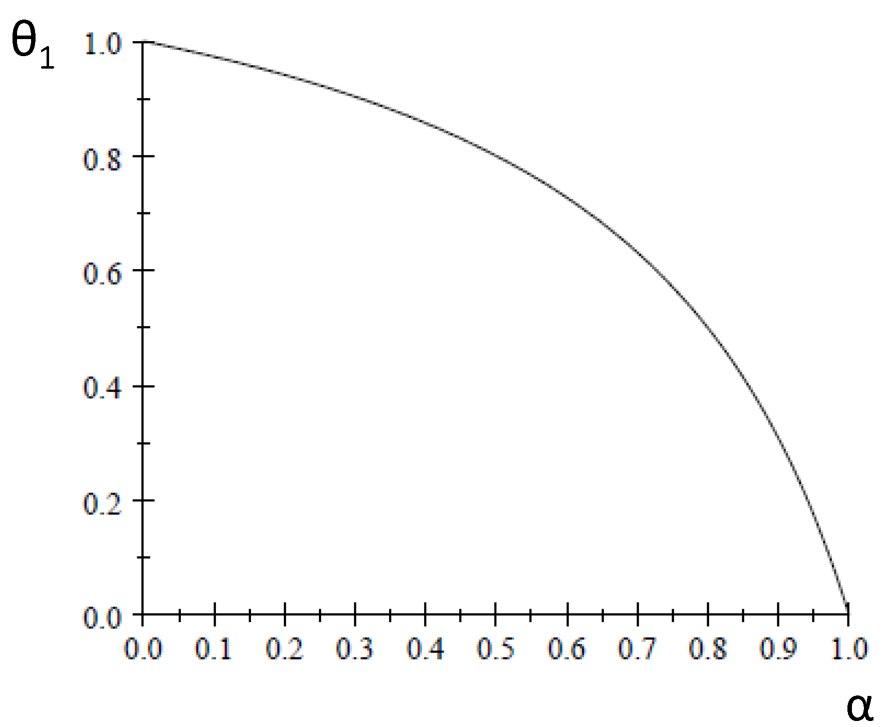
In order for this strategy combination to be an equilibrium, it must be the case that . Given the found values for and , this is the case if , or equivalently if . Note that is always between zero and one, given that . Figure 1 shows the parameter region where this equilibrium exists for ; it consists of all of the combinations above the curve.
Figure 1.
Parameter regions (mixed-strategy equilibrium below curve).

Note that ; hence, if we fix one of the parameters α or , the condition on the other parameter becomes more demanding as n increases.
The second type of equilibrium occurs when the minor players play a mixed strategy. In order forthis to happen, for a minor player i must be the same for and for (Corollary 5); hence:
Expected pay-offs computed at the beginning of the game depend on the mixed strategy of the minor players. Let λ be the probability that a minor player m proposes protocoalition (our symmetry assumption implies that all minor players must use the same λ). The expression for is quite simple, since the expected pay-off for Player 1 conditional on being in a protocoalition of type is irrespective of who proposed it.
The equation for is in principle more lengthy, but can easily be simplified. Each minor player is selected with probability to be formateur, and then proposes coalition with probability λ (in which case, its pay-off is ) and coalition with probability (in which case, its pay-off is . The minor player also receives proposals from the apex player with probability (given that the apex player is selected to be formateur with probability and proposes to each of the available minor players with the same probability) and from other minor players with probability (given that each minor player is selected as formateur with probability , there are other minor players, and each of them proposes the minor player coalition with probability ). If we note that expected pay-offs given that a protocoalition is formed do not depend on which member of the coalition was the formateur, and that, by assumption, in this type of equilibrium, minor players are indifferent between the two types of minimal winning coalitions available, collecting terms and using the indifference condition , a minor player’s expected pay-off is reduced to its probability of being in the coalition times its expected pay-off conditional on being in thecoalition, .
Solving the system of three equations, we find:
Since and , the expression for λ is always less than one. In order for , we need (when , we have , and the minor players never propose to the apex player, even though a protocoalition with the apex player is just as desirable as a protocoalition with the other minor players).
One thing to note is that and do not depend on . As for α, (the opposite is true for , since ).
Conflicts of Interest
The author declares no conflict of interest.
References
- Baron, D.; Ferejohn, J. Bargaining in legislatures. Am. Polit. Sci. Rev. 1989, 83, 1181–1206. [Google Scholar] [CrossRef]
- Eraslan, H.; McLennan, A. Uniqueness of stationary equilibrium payoffs in coalitional bargaining. J. Econ. Theory 2013, 148, 2195–2222. [Google Scholar] [CrossRef]
- Selten, R. A noncooperative model of characteristic function bargaining. In Essays in Game Theory and Mathematical Economics in Honor of Oskar Morgenstern; Böhm, V., Nachtkamp, H., Eds.; Bibliographisches Institut: Mannheim, Germany, 1981. [Google Scholar]
- Chatterjee, K.; Dutta, B.; Ray, D.; Sengupta, K. A noncooperative theory of coalitional bargaining. Rev. Econ. Stud. 1993, 60, 463–477. [Google Scholar] [CrossRef]
- Diermeier, D.; Merlo, A. Government turnover in parliamentary democracies. J. Econ. Theory 2000, 94, 46–79. [Google Scholar] [CrossRef]
- Jackson, M.; Moselle, B. Coalition and party formation in a legislative voting game. J. Econ. Theory 2002, 103, 49–87. [Google Scholar] [CrossRef]
- Carrubba, C.; Volden, C. Coalitional politics and logrolling in legislative institutions. Am. J. Polit. Sci. 2000, 44, 261–277. [Google Scholar] [CrossRef]
- Eguia, J. Endogenous parties in an assembly. Am. J. Polit. Sci. 2011, 73, 111–135. [Google Scholar] [CrossRef]
- Baron, D.; Diermeier, D. Elections, governments and parliaments in proportional representation systems. Q. J. Econ. 2001, 116, 933–967. [Google Scholar] [CrossRef]
- Diermeier, D.; Eraslan, H.; Merlo, A. A structural model of government formation. Econometrica 2003, 71, 27–70. [Google Scholar] [CrossRef]
- Breitmoser, Y. Protocoalition bargaining and the core. Econ. Theory 2012, 51, 581–599. [Google Scholar] [CrossRef] [Green Version]
- Karos, D. Coalition formation in general apex games under monotonic power indices. Games Econ. Behav. 2014, 87, 239–252. [Google Scholar] [CrossRef]
- Kalandrakis, T. Proposal rights and political power. Am. J. Polit. Sci. 2006, 50, 441–448. [Google Scholar] [CrossRef]
- Diermeier, D.; Merlo, A. An empirical investigation of coalitional bargaining procedures. J. Public Econ. 2004, 88, 783–797. [Google Scholar] [CrossRef]
- Baron, D.; Kalai, E. The simplest equilibrium of a majority-rule division game. J. Econ. Theory 1993, 61, 290–301. [Google Scholar] [CrossRef]
- Seidmann, D.; Winter, E.; Pavlov, E. The formateur’s role in government formation. Econ. Theory 2007, 31, 427–445. [Google Scholar] [CrossRef]
- Okada, A. A noncooperative coalitional bargaining game with random proposers. Games Econ. Behav. 1996, 16, 97–108. [Google Scholar] [CrossRef]
- Binmore, K. Perfect equilibria in bargaining models. In The Economics of Bargaining; Binmore, K., Dasgupta, P., Eds.; Blackwell: Oxford, UK, 1987. [Google Scholar]
- Binmore, K.; Rubinstein, A.; Wolinsky, A. The Nash bargaining solution in economic modelling. Rand J. Econ. 1986, 17, 176–188. [Google Scholar] [CrossRef]
- Rubinstein, A.; Wolinsky, A. Equilibrium in a market with sequential bargaining. Econometrica 1985, 53, 1133–1150. [Google Scholar] [CrossRef]
- Aumann, R.; Drèze, J. Cooperative games with coalition structures. Int. J. Game Theory 1974, 3, 217–237. [Google Scholar] [CrossRef]
- Laruelle, A.; Valenciano, F. Noncooperative foundations of bargaining power in committees and the Shapley-Shubik index. Games Econ. Behav. 2008, 63, 341–353. [Google Scholar] [CrossRef]
- Montero, M. Noncooperative bargaining in apex games and the kernel. Games Econ. Behav. 2002, 41, 309–321. [Google Scholar] [CrossRef]
- Eraslan, H. Uniqueness of stationary equilibrium payoffs in the Baron-Ferejohn model. J. Econ. Theory 2002, 103, 11–30. [Google Scholar] [CrossRef]
- Kawamori, T. Players’ patience and equilibrium payoffs in the Baron-Ferejohn model. Econ. Bull. 2005, 3, 1–7. [Google Scholar]
- Felsenthal, D.; Machover, M. The Measurement of Voting Power: Theory and Practice, Problems and Paradoxes; Edward Elgar Publishing: Cheltenham, UK, 1998. [Google Scholar]
- Schmeidler, D. The nucleolus of a characteristic function game. SIAM J. Appl. Math. 1969, 17, 1163–1170. [Google Scholar] [CrossRef]
- Grotte, J. Computation of and Observations on the Nucleolus, the Normalized Nucleolus and the Central Games. Master’s thesis, Cornell University, Ithaca, NY, USA, 1970. [Google Scholar]
- Montero, M. Noncooperative foundations of the nucleolus in majority games. Games Econ. Behav. 2006, 54, 380–397. [Google Scholar] [CrossRef]
- Browne, E.; Franklin, M. Aspects of coalition payoffs in European parliamentary democracies. Am. Polit. Sci. Rev. 1973, 67, 453–469. [Google Scholar] [CrossRef]
- Warwick, P.; Druckman, J. The portfolio allocation paradox: An investigation into the nature of a very strong but puzzling relationship. Eur. J. Polit. Res. 2006, 45, 635–665. [Google Scholar] [CrossRef]
- Snyder, J.; Ting, M.; Ansolabehere, S. Legislative bargaining under weighted voting. Am. Econ. Rev. 2005, 95, 981–1004. [Google Scholar] [CrossRef]
- Laver, M.; de Marchi, S.; Mutlu, H. Negotiations in legislatures over government formation. Public Choice 2011, 147, 285–304. [Google Scholar] [CrossRef]
- Von Neumann, J.; Morgenstern, O. Theory of Games and Economic Behavior; Princeton University Press: Princeton, NJ, USA, 1944. [Google Scholar]
- McKelvey, R.; Ordeshook, P.; Winer, M. The competitive solution for n-peron games without transferable utility, with an application to committee games. Am. Polit. Sci. Rev. 1978, 72, 599–615. [Google Scholar] [CrossRef]
- Davis, M.; Maschler, M. The kernel of a cooperative game. Naval Res. Log. Q. 1965, 12, 223–259. [Google Scholar] [CrossRef]
- Fréchette, G.; Kagel, J.; Morelli, M. Behavioral identification in coalitional bargaining: An experimental analysis of demand bargaining and alternating offers. Econometrica 2005, 73, 1893–1937. [Google Scholar] [CrossRef]
- 1This model has lots of applications and extensions. A fairly comprehensive list can be found in Eraslan and McLennan [2].
- 3Diermeier and Merlo [5] (p. 51) define a protocoalition as a set of parties that agree to talk to each other about forming a government together.
- 4Jackson and Moselle [6] examine the formation of political parties in a legislative bargaining situation, where a party is defined as a binding agreement to make the same proposal when recognized and to vote for each other’s proposals. Other papers that model political parties as voting blocs include Carrubba and Volden [7] and Eguia [8].
- 5Jackson and Moselle [6] assume that the surplus is split among party members according to the Nash bargaining solution, taking as disagreement outcome the situation with no political parties. In contrast, the present model has a breakdown outcome that incorporates the possibility of forming new coalitions if the current protocoalition fails.
- 6A recent paper by Karos [12] analyses coalition formation in apex games using core stability under a fixed pay-off division rule as a solution concept.
- 7The seat distribution in the German Bundestag often corresponds to an apex game. For example, after the 2013 federal election, the seat distribution was CDU/CSU311, SPD193, Bündnis 90/Die Grünen 64 and Die Linke 63. Assuming a majority of 316, a minimal winning coalition can be formed by CDU/CSU with either of the three other parties or by the other three parties together.
- 8The central role of proposal rights in determining expected equilibrium pay-offs in the original Baron-Ferejohn model has been established by Kalandrakis [13].
- 9Diermeier and Merlo [14] find empirical support for the random selection of formateurs in several European countries.
- 10The assumption of sequential moves may be replaced by simultaneous moves with the additional assumption that players behave as if they are pivotal (see Baron and Kalai [15]). The role of this assumption is to rule out equilibria in which several players reject a profitable proposal just because they are not pivotal.
- 11Note that proposer selection is independent of which player was the formateur. Seidmann et al. [16] also separate the roles of the formateur and the proposer.
- 12Notice that equilibria in which several responders reject just because S is going to be rejected anyhow are ruled out by the fact that the players in S respond sequentially.
- 13If we relax this assumption, there may be equilibria where strategies are not symmetric (for example, the apex player may be more likely to propose a protocoalition with specific minor players), but it is still the case that all minor players have the same expected equilibrium pay-offs.
- 15Montero [23] shows that the mixed-strategy equilibrium region is also quite large in the original Baron-Ferejohn model for apex games.
- 17This comparative statics result is qualitatively similar to the donation paradox in power indices (see Felsenthal and Machover [26], Definition 7.8.3). According to Felsenthal and Machover, a donation paradox occurs when a player loses power as a result of a transfer of voting weight from another player. In the present paper, the minor players may be worse-off as a result of a transfer of proposing probability from the apex player.
- 18If several allocations minimize the maximum per capita excess, the set is refined until one allocation is identified.
- 19In the original Baron-Ferejohn model with general voting rules, Montero [29] shows that if the recognition probabilities coincide with the nucleolus, expected equilibrium pay-offs coincide with the nucleolus, as well.
- 20The Baron-Ferejohn model does not distinguish between formateur and proposer. The empirical literature tests for a formateur advantage, whereas the current paper predicts a proposer advantage. The model could be modified to allow the first proposer in a protocoalition to coincide with the formateur.
© 2015 by the authors; licensee MDPI, Basel, Switzerland. This article is an open access article distributed under the terms and conditions of the Creative Commons Attribution license (http://creativecommons.org/licenses/by/4.0/).
Share and Cite
MDPI and ACS Style
Montero, M. A Model of Protocoalition Bargaining with Breakdown Probability. Games 2015, 6, 39-56. https://0-doi-org.brum.beds.ac.uk/10.3390/g6020039
AMA Style
Montero M. A Model of Protocoalition Bargaining with Breakdown Probability. Games. 2015; 6(2):39-56. https://0-doi-org.brum.beds.ac.uk/10.3390/g6020039
Chicago/Turabian StyleMontero, Maria. 2015. "A Model of Protocoalition Bargaining with Breakdown Probability" Games 6, no. 2: 39-56. https://0-doi-org.brum.beds.ac.uk/10.3390/g6020039