Effective Elasticity Tensor of Fiber-Reinforced Orthorhombic Composite Materials with Fiber Distribution Parallel to Plane

Abstract

An orthogonal composite material $\mathsf{\Omega }$ with fibers consists of a matrix and orthothombic distribution fibers. In addition to the matrix properties, the fiber properties and the fiber volume fraction, the effective (macroscopic) elastic stress–strain constitutive relation of $\mathsf{\Omega }$ is related to the fiber direction distribution. Until now, there have been few papers that give an explicit formula of the macroscopic elastic stress–strain constitutive relation of $\mathsf{\Omega }$ with the effect of the fiber direction distribution. Taking the expanded coefficients of the Fourier series as the fiber direction distribution coefficients, we give a formula of the fiber direction distribution parallel to a plane computed through the fiber directions. By the self-consistent estimates, we derive an explicit formula of the macroscopic elastic stress–strain constitutive relation of $\mathsf{\Omega }$ with the fiber direction distribution coefficients. Since all tensors are represented in Kelvin notation, the macroscopic elastic stress–strain constitutive relation of $\mathsf{\Omega }$ can be derived and computed only by matrix manipulations. To check the explicit formula, we use the FEM computation to obtain the macroscopic elastic stress–strain relation of $\mathsf{\Omega }$ for three examples. The computational results of the explicit formula for the three examples are consistent with those of the FEM simulations.

1. Introduction

Materials play an important role in the development of the manufacturing industry. Composite materials have the important advantages of high specific strength, a strong damping capacity and high specific modulus and can be used as a substitute for traditional materials. In modern times, fiber-reinforced polymer composite materials have important applications in many industries due to their light weight, water resistance, high impact strength, environmental friendliness and other advantages [1,2,3,4,5]. Fiber-reinforced composite materials have better mechanical properties, wear resistance, impact resistance and fire resistance.

Hence, they are suitable in various fields, such as civil engineering, aerospace, highway construction, electric power construction and marine facilities [6,7,8]. Therefore, the research of fiber-reinforced composite materials is of great significance. The properties of nonhomogeneous materials under external forces depend on their internal structures. A fiber-reinforced composite material consists of a matrix and numerous fibers (cylindrical inclusions) in Figure 1. Composite materials with fibers belong to nonhomogeneous materials. Compared to composite materials with fibers, there are many papers regarding the macroscopic properties of sheet metals with the effects of the mesostructures. The mesostructures of sheet metals are mainly the crystalline orientation distribution.

The crystalline orientation distribution function (CDF) was used to give the probability density of finding a crystal with $\mathbf{R}$ on SO(3) [9,10,11]. The CDF is expanded under the Wigner D function bases [12,13]. The expanded coefficients (i.e., the texture coefficients) of the CDF under the Wigner D function bases were introduced into the constitutive relations of sheet metals through the Voigt assumption and the orientational averaging [14,15]. Under the Voigt assumption [16], all crystals in a polycrystal are assumed to have the same deformation.

For the Reuss assumption [17], the basic assumption is that all crystals in a polycrystal have the same stress state. To ensure the traction and deformation’s continuity among crystals in a sense, a self-consistent estimate was introduced by Kröner [18,19]. Nemat-Nasser and Hori [20] studied the self-consistent estimates. Morris [21] obtained the macroscopic elastic stress–strain relation of sheet metals by self-consistent estimates. Huang [22] derived the macroscopic elastic stress–strain constitutive relation of sheet metals with the texture coefficients by the self-consistent estimates.

Huang [23] gave the elastic constitutive relations of polycrystals by the perturbation approach. Huang and Man [24] introduced a new Hosford yield function of sheet metals with the effect of the texture coefficients. Dong et al. [25] discussed the macroscopic elastic constitutive relation of a fiber-reinforced composite material by the self-consistent estimates. Through experiments, Mohankumar et al. [26] evaluated the effect of fiber orientation on the tribological properties of the TAFR composites. The 20% TAFR composites showed relatively better mechanical properties.

Hashin and Rosen [27] and Hashin [28] presented the macroscopic elastic properties of fiber-reinforced materials. Hill [29,30] derived the stress-stain relation of fiber-strengthened materials. The mesostructures of fiber-reinforced materials are the fiber direction distribution. Tian et al. [31] used a multi-scale numerical model to study the global buckling and local response of composite cylindrical shells with trapezoidal corrugated cores. However, there are few papers to give the explicit formula of the macroscopic elastic stress–strain constitutive relation on fiber-reinforced composite materials with the effect of the fiber direction distribution.

We use $\mathsf{\Omega }$ to denote a fiber reinforced orthogonal composite material. In Section 2, using the fiber direction distribution coefficients $W_{2m}$ of the Fourier series to present the fiber direction distribution function, we give a computational Formula (11) with fiber direction distribution coefficients $W_{2m}$. In Section 3, we present the stress, strain tensor, rotation and constitutive tensors in Kelvin notation. We study their rotation relations. In Section 4, we use the self-consistent estimates to derive an explicit Formula (64) of macroscopic elastic stress–strain constitutive relation $\widehat{\mathbf{C}}$ on $\mathsf{\Omega }$ with the fiber direction distribution coefficients.

The computation procedures of the explicit Formula (64) are simple since the Kelvin notation is used for denoting all these tensors. In Section 5, for checking the explicit formula, we use FEM to compute the macroscopic elastic stress–strain relation of the composite materials with fibers in three examples. The computational results of the three examples based on the explicit Formula (64) are consistent with those of FEM.

In this paper, we attempt to answer the following problems: (1) the determination of the fiber direction distribution coefficients $W_{2m}$ to the fiber direction distribution of $\mathsf{\Omega }$ has completeness; (2) the effect of the fiber direction distribution to $\widehat{\mathbf{C}}$ of $\mathsf{\Omega }$ can be given only via $W_2$ and $W_4$ in (11)${}_2$; and (3) the derivation and the computation of $\widehat{\mathbf{C}}$ in Kelvin notation can be completed by the linear algebra’s matrix manipulations.

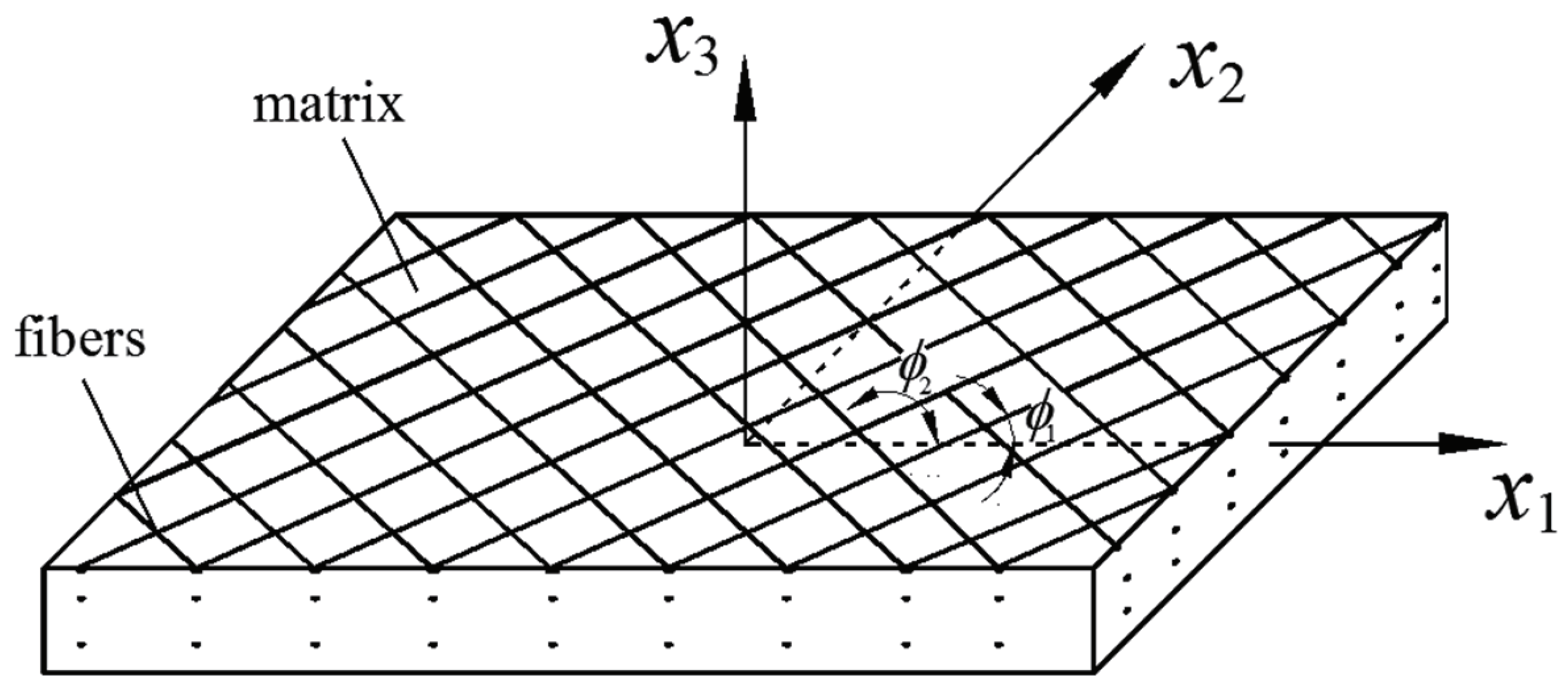
2. Fiber Direction Distribution of Fiber-Reinforced Orthogonal Composite Material

For a fixed Cartesian coordinate system $x_i$, a fiber-reinforced orthogonal composite material $\mathsf{\Omega }$ is given in Figure 1. The fiber-reinforced orthogonal composite material $\mathsf{\Omega }$ consists of the matrix ${\mathsf{\Omega }}^{\left(0\right)}$ and the orthogonal direction distribution fibers ${\mathsf{\Omega }}^{\left(1\right)}$, where ${\mathsf{\Omega }}^{\left(0\right)}$ and ${\mathsf{\Omega }}^{\left(1\right)}$ denote the domains of the matrix and the fibers, respectively, with $\mathsf{\Omega }={\mathsf{\Omega }}^{\left(0\right)}\cup {\mathsf{\Omega }}^{\left(1\right)}$. As $\mathsf{\Omega }$ is orthogonal, the three axes of the fixed coordinate system are assumed to agree with the orthogonal symmetric axes of $\mathsf{\Omega }$. ${\mathsf{\Omega }}^{\left(1\right)}$$={\cup }_{p=1}^n{\mathsf{\Omega }}_{{\varphi }_p}^{\left(1\right)}$ consist of the fibers parallel to a plane with n different directions ${\varphi }_p$ ($p=1,2,\cdots ,n$), where the fibers ${\mathsf{\Omega }}_{{\varphi }_p}^{\left(1\right)}$ have angle ${\varphi }_p$ with respect to $x_1$.

Use the fiber direction distribution function (FDF) $w\left(\varphi \right)$ to describe the probability density of finding that the fiber direction is $\varphi$ of in ${\mathsf{\Omega }}^{\left(1\right)}$. The description of the Fourier series to the FDF has completeness. The FDF $w\left(\varphi \right)$ can be expanded as an infinite series $w\left(\varphi \right)=\frac{1}{\pi }{\displaystyle \sum _{m=-\infty }^{\infty }}{c}_m{e}^{-im\varphi }$, where $\overline{m}\stackrel{\mathrm{def}}{=}-m$ and $c_{\overline{m}}=c_m^{*}$, $c_m^{*}$ is the complex conjugate of the complex number $c_m$, and the expanded coefficients $c_m$ are the fiber direction distribution coefficients. The condition $c_{\overline{m}}=c_m^{*}$ makes that $w\left(\varphi \right)$ is a real function because

$$c_m{e}^{-im\varphi }+c_{\overline{m}}{e}^{-i(-m)\varphi }=c_m{e}^{-im\varphi }+{\left(c_m{e}^{-im\varphi }\right)}^{*}=2Re\left(c_m{e}^{-im\varphi }\right).$$

(1)

Let ${\varphi }_p$ be the direction of the fibers ${\mathsf{\Omega }}_{{\varphi }_p}^{\left(1\right)}$. We should have $w\left({\varphi }_p\right)=w(\pi +{\varphi }_p)$ or $c_m{e}^{-im{\varphi }_p}=c_m{e}^{-im\pi }{e}^{-im{\varphi }_p}$ which leads to

$$c_m=0,m\in \mathrm{odd};c_m=c_m,m\in \mathrm{even}.$$

(2)

Considering the restriction (2), we express the FDF $w\left(\varphi \right)$ as follows:

$$w\left(\varphi \right)=\frac{1}{\pi }\sum _{m=-\infty }^{\infty }{c}_{2m}{e}^{-i2m\varphi },c_{2\overline{m}}=c_{2m}^{*}{c}_0=1.$$

(3)

There is ${\int }_0^{\pi }w\left(\varphi \right)d\varphi =1$ for any $c_{2m}$ by ${\int }_0^{\pi }{e}^{-i2m\varphi }d\varphi =0$ if $m\ne 0$. The term $e^{-i2m\varphi }$ ($m=0,1,2,\cdots$) constitute orthogonal bases

$${\int }_0^{\pi }{e}^{-i2m\varphi }{\left(e^{-i2n\varphi }\right)}^{*}d\varphi =\pi {\delta }_{mn}.$$

(4)

From (3) and (4), we know that the expanded coefficients (i.e., the fiber direction distribution coefficients $c_{2m}$) of the FDF under the basis $e^{-i2m\varphi }$ can be obtained by

$$c_{2m}={\int }_0^{\pi }w\left(\varphi \right){\left(e^{-i2m\varphi }\right)}^{*}d\varphi .$$

(5)

When all the fibers in $\mathsf{\Omega }$ are one direction ${\varphi }_p$, then

$$w\left(\varphi \right)=\delta (\varphi -{\varphi }_p),{\varphi }_p\in [0,\pi ).$$

(6)

By (5), the fiber direction distribution coefficients $c_{2m}\left({\varphi }_p\right)$ of $\mathsf{\Omega }$ with one direction ${\varphi }_p$ should be

$$c_{2m}\left({\varphi }_p\right)={\int }_0^{\pi }\delta (\varphi -{\varphi }_p){\left(e^{-i2m\varphi }\right)}^{*}d\varphi ={\left(e^{-i2m{\varphi }_p}\right)}^{*}=e^{i2m{\varphi }_p},$$

(7)

where the Dirac delta function $\delta (\varphi -{\varphi }_p)$ on [0, $\pi )$ satisfies ${\int }_0^{\pi }\delta (\varphi -{\varphi }_p)f\left(\varphi \right)d\varphi$$=f\left({\varphi }_p\right)$. For the fibers in $\mathsf{\Omega }$ having n directions ${\varphi }_p\in$[0, $\pi )$, the fiber direction distribution coefficients of $\mathsf{\Omega }$ are the volume average of $c_{2m}\left({\varphi }_p\right)$ ($p=1,2,\cdots ,n$) on all the fibers:

$$c_{2m}=\frac{1}{|{\mathsf{\Omega }}^{\left(1\right)}|}\sum _{p=1}^n\left|{\mathsf{\Omega }}_{{\varphi }_p}^{\left(1\right)}\right|e^{i2m{\varphi }_p}$$

(8)

by the definition of the FDF, where $|{\mathsf{\Omega }}^{\left(1\right)}|$ is the volume of domain ${\mathsf{\Omega }}^{\left(1\right)}$, $|{\mathsf{\Omega }}_{{\varphi }_p}^{\left(1\right)}|$ is the volume of domain ${\mathsf{\Omega }}_{{\varphi }_p}^{\left(1\right)}$, and ${\mathsf{\Omega }}_{{\varphi }_p}^{\left(1\right)}$ with ${\mathsf{\Omega }}^{\left(1\right)}={\cup }_{p=1}^n{\mathsf{\Omega }}_{{\varphi }_p}^{\left(1\right)}$ is the domain of the fibers on direction ${\varphi }_p$.

If the complex number $c_{2m}$ is expressed as

$$c_{2m}=W_{2m}+i{M}_{2m}(\mathrm{i}.\mathrm{e}.,W_{2m}=Re{c}_{2m},M_{2m}=Im{c}_{2m}),$$

(9)

From (1) and (9), we rewrite (3) into

$$\begin{array}{c}w\left(\varphi \right)=\frac{1}{\pi }+\frac{2}{\pi }\sum _{m=1}^{\infty }Re\left(c_{2m}{e}^{-i2m\varphi }\right)\\ =\frac{1}{\pi }+\frac{2}{\pi }\sum _{m=1}^{\infty }(W_{2m}cos2m\varphi +M_{2m}sin2m\varphi ).\end{array}$$

(10)

Since the fiber direction distribution of $\mathsf{\Omega }$ in Figure 1 is orthogonal, the fiber directions have ${\varphi }_p$ and $\pi -$${\varphi }_p$ in pairs (i.e., $|{\mathsf{\Omega }}_{{\varphi }_p}^{\left(1\right)}|=|{\mathsf{\Omega }}_{\pi -{\varphi }_p}^{\left(1\right)}\left|\right)$ where ${\varphi }_p\in [0,\frac{\pi }{2})$. Since $|{\mathsf{\Omega }}_{{\varphi }_p}^{\left(1\right)}|e^{i2m{\varphi }_p}+\left|{\mathsf{\Omega }}_{\pi -{\varphi }_p}^{\left(1\right)}\right|e^{i2m(\pi -{\varphi }_p)}$=$|{\mathsf{\Omega }}_{{\varphi }_p}^{\left(1\right)}|\left(e^{i2m{\varphi }_p}+e^{-i2m{\varphi }_p}\right)$ $=2|{\mathsf{\Omega }}_{{\varphi }_p}^{\left(1\right)}|cos2m{\varphi }_p$, we rewrite the fiber direction distribution function $w\left(\varphi \right)$ and the fiber direction distribution coefficients $W_{2m}$ ($c_{2m}$) in (10) and (8) for the fiber orthogonal composite material $\mathsf{\Omega }$ as follows

$$w\left(\varphi \right)=\frac{1}{\pi }+\frac{2}{\pi }\sum _{m=1}^{\infty }{W}_{2m}cos2m\varphi ,W_{2m}=\frac{1}{|{\mathsf{\Omega }}^{\left(1\right)}|}\sum _{p=1}^n\left|{\mathsf{\Omega }}_{{\varphi }_p}^{\left(1\right)}\right|cos2m{\varphi }_p,$$

(11)

where ${\varphi }_p$, $\varphi \in [0,\pi )$. The coefficients $W_{2m}$ of the FDF are determined by (11)${}_2$ and the fiber direction distribution angles ${\varphi }_p$ ($p=1,2,\cdots ,n$). The computational formula (11)${}_2$ is important.

3. Representation of Tensors in Kelvin Notation

Let $\mathring{\mathbf{\sigma }}$ and $\mathring{\mathbf{\epsilon }}$ denote the stress and the strain, respectively, acting on element ${\mathcal{E}}_{\mathbf{I}}$

$$\mathring{\mathbf{\sigma }}=\left[\begin{array}{ccc}{\mathring{T}}_{11}& {\mathring{T}}_{12}& {\mathring{T}}_{13}\\ {\mathring{T}}_{12}& {\mathring{T}}_{22}& {\mathring{T}}_{23}\\ {\mathring{T}}_{13}& {\mathring{T}}_{23}& {\mathring{T}}_{33}\end{array}\right],\mathring{\mathbf{\epsilon }}=\left[\begin{array}{ccc}{\mathring{E}}_{11}& {\mathring{E}}_{12}& {\mathring{E}}_{13}\\ {\mathring{E}}_{12}& {\mathring{E}}_{22}& {\mathring{E}}_{23}\\ {\mathring{E}}_{13}& {\mathring{E}}_{23}& {\mathring{E}}_{33}\end{array}\right].$$

(12)

When the element ${\mathcal{E}}_{\mathbf{I}}$ with its external forces rotates $\varphi$ about $x_3$ and ${\mathcal{E}}_{\mathbf{I}}$ becomes ${\mathcal{E}}_{\mathbf{R}}$, the stress $\mathbf{\sigma }$ and the stress $\mathbf{\epsilon }$ of ${\mathcal{E}}_{\mathbf{R}}$ become

$$\mathbf{\sigma }=\left[\begin{array}{ccc}{T}_{11}& T_{12}& T_{13}\\ T_{12}& T_{22}& T_{23}\\ T_{13}& T_{23}& T_{33}\end{array}\right]{=\mathbf{R}\mathring{\mathbf{\sigma }}\mathbf{R}}^T,\mathbf{\epsilon }=\left[\begin{array}{ccc}{E}_{11}& E_{12}& E_{13}\\ E_{12}& E_{22}& E_{23}\\ E_{13}& E_{23}& E_{33}\end{array}\right]{=\mathbf{R}\mathring{\mathbf{\epsilon }}\mathbf{R}}^T,$$

(13)

where $\mathbf{R}$ is a rotation tensor about axis $x_3$

$$\mathbf{R}=\left[\begin{array}{ccc}cos\varphi & -sin\varphi & 0\\ sin\varphi & cos\varphi & 0\\ 0& 0& 1\end{array}\right].$$

(14)

By the symmetries $T_{ij}=T_{ji}$ and ${\mathring{T}}_{ij}={\mathring{T}}_{ji}$ of stress components in $\mathbf{\sigma }$ and $\mathring{\mathbf{\sigma }}$, the relation ${\mathbf{\sigma }=\mathbf{R}\mathring{\mathbf{\sigma }}\mathbf{R}}^T$ (or ${\mathbf{\epsilon }=\mathbf{R}\mathring{\mathbf{\epsilon }}\mathbf{R}}^T$) constitutes six equations between $T_{ij}$ and ${\mathring{T}}_{ij}$. The six equations on $T_{ij}$ and ${\mathring{T}}_{ij}$ (or $E_{ij}$ and ${\mathring{E}}_{ij}$) can be written into

$$\mathbf{T}=\mathbf{Q}\mathring{\mathbf{T}},\mathbf{E}=\mathbf{Q}\mathring{\mathbf{E}},$$

(15)

where $\mathbf{T}$, $\mathring{\mathbf{T}}$, $\mathbf{E}$ and $\mathring{\mathbf{E}}$ are the stress tensor and the strain tensor in Kelvin notation [32]

$$\begin{array}{cc}\hfill \mathring{\mathbf{T}}& ={[{\mathring{T}}_{11},{\mathring{T}}_{22},{\mathring{T}}_{33},\sqrt{2}{\mathring{T}}_{23},\sqrt{2}{\mathring{T}}_{13},\sqrt{2}{\mathring{T}}_{12}]}^T,\hfill \\ \hfill \mathbf{T}& ={[T_{11},T_{22},T_{33},\sqrt{2}{T}_{23},\sqrt{2}{T}_{13},\sqrt{2}{T}_{12}]}^T,\hfill \\ \hfill \mathring{\mathbf{E}}& ={[{\mathring{E}}_{11},{\mathring{E}}_{22},{\mathring{E}}_{33},\sqrt{2}{\mathring{E}}_{23},\sqrt{2}{\mathring{E}}_{13},\sqrt{2}{\mathring{E}}_{12}]}^T,\hfill \\ \hfill \mathbf{E}& ={[E_{11},E_{22},E_{33},\sqrt{2}{E}_{23},\sqrt{2}{E}_{13},\sqrt{2}{E}_{12}]}^T.\hfill \end{array}$$

(16)

$\mathbf{Q}$ is the rotation tensor in Kelvin notation

$$\mathbf{Q}=\left[\begin{array}{cccccc}{cos}^2\varphi & {sin}^2\varphi & 0& 0& 0& -\frac{sin2\varphi }{\sqrt{2}}\\ {sin}^2\varphi & {cos}^2\varphi & 0& 0& 0& \frac{sin2\varphi }{\sqrt{2}}\\ 0& 0& 1& 0& 0& 0\\ 0& 0& 0& cos\varphi & sin\varphi & 0\\ 0& 0& 0& -sin\varphi & cos\varphi & 0\\ \frac{sin2\varphi }{\sqrt{2}}& -\frac{sin2\varphi }{\sqrt{2}}& 0& 0& 0& cos2\varphi \end{array}\right].$$

(17)

$\mathbf{Q}$ is orthogonal, i.e.,

$${\mathbf{Q}}^T={\mathbf{Q}}^{-1},det\mathbf{Q}=1.$$

(18)

For the Voigt notation, the stress–strain relation is

$$\left[\begin{array}{c}{T}_{11}\\ T_{22}\\ T_{33}\\ T_{23}\\ T_{13}\\ T_{12}\end{array}\right]=\left[\begin{array}{cccccc}{\overline{c}}_{11}& {\overline{c}}_{12}& {\overline{c}}_{13}& {\overline{c}}_{14}& {\overline{c}}_{15}& {\overline{c}}_{16}\\ {\overline{c}}_{12}& {\overline{c}}_{22}& {\overline{c}}_{23}& {\overline{c}}_{24}& {\overline{c}}_{25}& {\overline{c}}_{26}\\ {\overline{c}}_{13}& {\overline{c}}_{23}& {\overline{c}}_{33}& {\overline{c}}_{34}& {\overline{c}}_{35}& {\overline{c}}_{36}\\ {\overline{c}}_{14}& {\overline{c}}_{24}& {\overline{c}}_{34}& {\overline{c}}_{44}& {\overline{c}}_{45}& {\overline{c}}_{46}\\ {\overline{c}}_{15}& {\overline{c}}_{25}& {\overline{c}}_{35}& {\overline{c}}_{45}& {\overline{c}}_{55}& {\overline{c}}_{56}\\ {\overline{c}}_{16}& {\overline{c}}_{26}& {\overline{c}}_{36}& {\overline{c}}_{46}& {\overline{c}}_{56}& {\overline{c}}_{66}\end{array}\right]\left[\begin{array}{c}{E}_{11}\\ E_{22}\\ E_{33}\\ 2E_{23}\\ 2E_{13}\\ 2E_{12}\end{array}\right]$$

(19)

for elastic anisotropic materials. For Kelvin notation, we rewrite the stress–strain relation (19) into [32]

$$\left[\begin{array}{c}{T}_{11}\\ T_{22}\\ T_{33}\\ \sqrt{2}{T}_{23}\\ \sqrt{2}{T}_{13}\\ \sqrt{2}{T}_{12}\end{array}\right]=\left[\begin{array}{cccccc}{\overline{c}}_{11}& {\overline{c}}_{12}& {\overline{c}}_{13}& \sqrt{2}{\overline{c}}_{14}& \sqrt{2}{\overline{c}}_{15}& \sqrt{2}{\overline{c}}_{16}\\ {\overline{c}}_{12}& {\overline{c}}_{22}& {\overline{c}}_{23}& \sqrt{2}{\overline{c}}_{24}& \sqrt{2}{\overline{c}}_{25}& \sqrt{2}{\overline{c}}_{26}\\ {\overline{c}}_{13}& {\overline{c}}_{23}& {\overline{c}}_{33}& \sqrt{2}{\overline{c}}_{34}& \sqrt{2}{\overline{c}}_{35}& \sqrt{2}{\overline{c}}_{36}\\ \sqrt{2}{\overline{c}}_{14}& \sqrt{2}{\overline{c}}_{24}& \sqrt{2}{\overline{c}}_{34}& 2{\overline{c}}_{44}& 2{\overline{c}}_{45}& 2{\overline{c}}_{46}\\ \sqrt{2}{\overline{c}}_{15}& \sqrt{2}{\overline{c}}_{25}& \sqrt{2}{\overline{c}}_{35}& 2{\overline{c}}_{45}& 2{\overline{c}}_{55}& 2{\overline{c}}_{56}\\ \sqrt{2}{\overline{c}}_{16}& \sqrt{2}{\overline{c}}_{26}& \sqrt{2}{\overline{c}}_{36}& 2{\overline{c}}_{46}& 2{\overline{c}}_{56}& 2{\overline{c}}_{66}\end{array}\right]\left[\begin{array}{c}{E}_{11}\\ E_{22}\\ E_{33}\\ \sqrt{2}{E}_{23}\\ \sqrt{2}{E}_{13}\\ \sqrt{2}{E}_{12}\end{array}\right]$$

(20)

whose six linear equations are the same as those of (19).

The stress–strain relation of ${\mathcal{E}}_{\mathbf{I}}$ is $\mathring{\mathbf{T}}=\mathring{\mathbf{C}}\mathring{\mathbf{E}}$ in Kelvin notation. After ${\mathcal{E}}_{\mathbf{I}}$ rotates $\varphi$ about $x_3$ and becomes ${\mathcal{E}}_{\mathbf{R}}$, the elastic stress–strain constitutive relation $\mathbf{C}$ of ${\mathcal{E}}_{\mathbf{R}}$ in Kelvin notation is

$$\mathbf{C}=\mathbf{Q}\mathring{\mathbf{C}}{\mathbf{Q}}^T$$

(21)

by (15) and (18).

The stress–strain relation (19) under Voigt notation is often used. However, the constitutive representation (20) in Kelvin notation has advantages because of the relations (15) and (21). The Kelvin notation makes that the derivation of the macroscopic elastic stress–strain constitutive relation (64) can be derived only via matrix computations.

4. Self-Consistent Estimates and Application in Fiber Orthogonal Composite Material $\mathsf{\Omega }$

4.1. Local and Macroscopic Elastic Stress-Strian Relation of $\mathsf{\Omega }$

The local stress and strain tensor in Kelvin notation are denoted by $\mathbf{T}\left(\mathbf{x}\right)$ and $\mathbf{E}\left(\mathbf{x}\right)$, respectively. The local constitutive relation is

$$\mathbf{T}\left(\mathbf{x}\right)={\mathbf{C}}^{\left(\beta \right)}\mathbf{E}\left(\mathbf{x}\right),\mathbf{x}\in {\mathsf{\Omega }}^{\left(\beta \right)}(\beta =0,1),$$

(22)

where ${\mathbf{C}}^{\left(0\right)}$ and ${\mathbf{C}}^{\left(1\right)}$ are the local elastic stress–strain relation for $\mathbf{x}\in {\mathsf{\Omega }}^{\left(0\right)}$ and $\mathbf{x}\in {\mathsf{\Omega }}^{\left(1\right)}={\cup }_{p=1}^n{\mathsf{\Omega }}_{{\varphi }_p}^{\left(1\right)}$, respectively. Let

$$f_0=\frac{|{\mathsf{\Omega }}^{\left(0\right)}|}{\left|\mathsf{\Omega }\right|},f_1=\frac{|{\mathsf{\Omega }}^{\left(1\right)}|}{\left|\mathsf{\Omega }\right|},$$

(23)

where $\left|\mathsf{\Omega }\right|$ and $|{\mathsf{\Omega }}^{\left(1\right)}|$ are the volumes of the matrix $\mathsf{\Omega }$ and the fibers ${\mathsf{\Omega }}^{\left(1\right)}$, respectively, $f_0$ is the matrix volume fraction, and $f_1$ is the fiber volume fraction, and $f_0+f_1=1$.

The average stress tensor $\widehat{\mathbf{T}}$ and the average strain tensor $\widehat{\mathbf{E}}$ of $\mathsf{\Omega }$ are given by

$$\widehat{\mathbf{T}}=\frac{1}{\left|\mathsf{\Omega }\right|}{\int }_{\mathsf{\Omega }}\mathbf{T}\left(\mathbf{x}\right)d\mathbf{x},\widehat{\mathbf{E}}=\frac{1}{\left|\mathsf{\Omega }\right|}{\int }_{\mathsf{\Omega }}\mathbf{E}\left(\mathbf{x}\right)d\mathbf{x}$$

(24)

respectively, where $d\mathbf{x}=d{x}_{1}d{x}_{2}d{x}_3$. The macroscopic elastic stress–strain constitutive relation $\widehat{\mathbf{C}}$ of $\mathsf{\Omega }$ is defined by

$$\widehat{\mathbf{T}}=\widehat{\mathbf{C}}\widehat{\mathbf{E}}.$$

(25)

In this paper, all tensors (e.g., $\mathbf{Q}$, $\widehat{\mathbf{C}}$, $\widehat{\mathbf{T}}$ and $\widehat{\mathbf{E}}$) are presented in Kelvin notation as shown in (16), (17) and (20). The macroscopic elastic stress–strain constitutive relation $\widehat{\mathbf{C}}$ of $\mathsf{\Omega }$ is important because the properties of $\mathsf{\Omega }$ are macroscopically like a homogeneous orthogonal material.

4.2. Self-Consistent Estimates for $\mathsf{\Omega }$

To keep that traction and displacement continuity among the matrix and the fibers in the fiber orthogonal composite material $\mathsf{\Omega }$ in a certain sense, we employ the self-consistent method based on eigenstrain [22] to compute the macroscopic elastic stress–strain constitutive relation of $\mathsf{\Omega }$.

Let us take the local elastic stress–strain constitutive relation ${\mathbf{C}}^{\left(0\right)}$ of the matrix ${\mathsf{\Omega }}^{\left(0\right)}$ as the reference material. Under the prescribed stress tensor $\widehat{\mathbf{T}}$, the reference material ${\mathbf{C}}^{\left(0\right)}$ has the elastic strain ${\mathbf{E}}^e$ [22]:

$$\widehat{\mathbf{T}}={\mathbf{C}}^{\left(0\right)}{\mathbf{E}}^e.$$

(26)

For the local constitutive relation of the fibers ${\mathsf{\Omega }}^{\left(1\right)}$ in (22), we employ the inclusion equivalence [20,22,33] to have

$$\begin{array}{c}\hfill \mathbf{T}\left(\mathbf{x}\right)={\mathbf{C}}^{\left(1\right)}\mathbf{E}\left(\mathbf{x}\right)={\mathbf{C}}^{\left(0\right)}\left[\mathbf{E}\left(\mathbf{x}\right)-\mathbf{H}\left(\mathbf{x}\right)\right],\\ \hfill \mathbf{H}\left(\mathbf{x}\right)=-{\left({\mathbf{C}}^{\left(0\right)}\right)}^{-1}\left({\mathbf{C}}^{\left(1\right)}-{\mathbf{C}}^{\left(0\right)}\right)\mathbf{E}\left(\mathbf{x}\right),\mathbf{x}\in {\mathsf{\Omega }}^{\left(1\right)},\end{array}$$

(27)

where $\mathbf{H}\left(\mathbf{x}\right)$ is the equivalent eigenstrain tensor of the fibers. The equivalent relation ${\mathbf{C}}^{\left(1\right)}\mathbf{E}\left(\mathbf{x}\right)={\mathbf{C}}^{\left(0\right)}\left(\mathbf{E}\left(\mathbf{x}\right)-\mathbf{H}\left(\mathbf{x}\right)\right)$ in (27) shows that the local elastic stress–strain constitutive relation ${\mathbf{C}}^{\left(1\right)}$ of the fibes ${\mathsf{\Omega }}^{\left(1\right)}$ is transfered into the reference material ${\mathbf{C}}^{\left(0\right)}$ when we increase an eigenstrain tensor $\mathbf{H}\left(\mathbf{x}\right)$ in ${\mathsf{\Omega }}^{\left(1\right)}$.

From the equivalence relation (27), the average stress $\widehat{\mathbf{T}}$ of $\mathsf{\Omega }$ should be

$$\begin{array}{cc}\hfill \widehat{\mathbf{T}}& =\frac{f_0}{|{\mathsf{\Omega }}^{\left(0\right)}|}{\int }_{{\mathsf{\Omega }}^{\left(0\right)}}\mathbf{T}\left(\mathbf{x}\right)d\mathbf{x}+\frac{f_1}{|{\mathsf{\Omega }}^{\left(1\right)}|}{\int }_{{\mathsf{\Omega }}^{\left(1\right)}}\mathbf{T}\left(\mathbf{x}\right)d\mathbf{x}\hfill \\ \hfill & ={\mathbf{C}}^{\left(0\right)}\left(\frac{f_0}{|{\mathsf{\Omega }}^{\left(0\right)}|}{\int }_{{\mathsf{\Omega }}^{\left(0\right)}}\mathbf{E}\left(\mathbf{x}\right)d\mathbf{x}+\frac{f_1}{|{\mathsf{\Omega }}^{\left(1\right)}|}{\int }_{{\mathsf{\Omega }}^{\left(1\right)}}(\mathbf{E}\left(\mathbf{x}\right)d\mathbf{x}-\mathbf{H}\left(\mathbf{x}\right))d\mathbf{x}\right)\hfill \\ \hfill & ={\mathbf{C}}^{\left(0\right)}\left(f_0{\tilde{\mathbf{E}}}^{\left(0\right)}+f_1({\tilde{\mathbf{E}}}^{\left(1\right)}-{\tilde{\mathbf{H}}}^{\left(1\right)})\right)={\mathbf{C}}^{\left(0\right)}(\widehat{\mathbf{E}}-\widehat{\mathbf{H}})\hfill \end{array}$$

(28)

with

$$\widehat{\mathbf{E}}=f_0{\tilde{\mathbf{E}}}^{\left(0\right)}+f_1{\tilde{\mathbf{H}}}^{\left(1\right)},\widehat{\mathbf{H}}=f_0{\tilde{\mathbf{H}}}^{\left(0\right)}+f_1{\tilde{\mathbf{H}}}^{\left(1\right)}=f_1{\tilde{\mathbf{H}}}^{\left(1\right)},$$

(29)

$${\tilde{\mathbf{E}}}^{\left(0\right)}=\frac{1}{|{\mathsf{\Omega }}^{\left(0\right)}|}{\int }_{{\mathsf{\Omega }}^{\left(0\right)}}\mathbf{E}\left(\mathbf{x}\right)d\mathbf{x},{\tilde{\mathbf{E}}}^{\left(1\right)}=\frac{1}{|{\mathsf{\Omega }}^{\left(1\right)}|}{\int }_{{\mathsf{\Omega }}^{\left(1\right)}}\mathbf{E}\left(\mathbf{x}\right)d\mathbf{x},$$

(30)

$${\tilde{\mathbf{H}}}^{\left(0\right)}=\frac{1}{|{\mathsf{\Omega }}^{\left(0\right)}|}{\int }_{{\mathsf{\Omega }}^{\left(0\right)}}\mathbf{0}d\mathbf{x}=\mathbf{0},{\tilde{\mathbf{H}}}^{\left(1\right)}=\frac{1}{|{\mathsf{\Omega }}^{\left(1\right)}|}{\int }_{{\mathsf{\Omega }}^{\left(1\right)}}\mathbf{H}\left(\mathbf{x}\right)d\mathbf{x},$$

(31)

where $\widehat{\mathbf{E}}$ is the average strain of $\mathsf{\Omega }$, $\widehat{\mathbf{H}}$ is the average equivalent eigenstrain of $\mathsf{\Omega }$,${\tilde{\mathbf{E}}}^{\left(0\right)}$ and ${\tilde{\mathbf{E}}}^{\left(1\right)}$ are the average strains of ${\mathsf{\Omega }}^{\left(0\right)}$ and ${\mathsf{\Omega }}^{\left(1\right)}$, respectively, ${\tilde{\mathbf{H}}}^{\left(0\right)}=\mathbf{0}$ and ${\tilde{\mathbf{H}}}^{\left(1\right)}$ are the average equivalent eigenstrain of ${\mathsf{\Omega }}^{\left(0\right)}$ and ${\mathsf{\Omega }}^{\left(1\right)}$, respectively.

As of $\widehat{\mathbf{T}}$ being a given stress tensor, the relation of (28) and (26) reads

$$\widehat{\mathbf{E}}={\mathbf{E}}^e+\widehat{\mathbf{H}}.$$

(32)

To obtain the macroscopic elasticity relation $\widehat{\mathbf{T}}=\widehat{\mathbf{C}}\widehat{\mathbf{E}}$ of $\mathsf{\Omega }$ from (28) and (32), one more relation among $\widehat{\mathbf{E}}$, ${\mathbf{E}}^e$ and $\widehat{\mathbf{H}}$ is needed.

Consider a fiber ${\mathcal{F}}_{\varphi }$$\subset {\mathsf{\Omega }}_{\varphi }^{\left(1\right)}$ with $\varphi$. If the strain $\mathbf{E}\left(\mathbf{x}\right)$ of ${\mathcal{F}}_{\varphi }$ is $\widehat{\mathbf{E}}={\mathbf{E}}^e+\widehat{\mathbf{H}}$ in (32), there will be no perturbation strain field and no perturbation stress field in ${\mathcal{F}}_{\varphi }$ and $\mathsf{\Omega }$ in a sense. Otherwise, the local strain of ${\mathcal{F}}_{\varphi }$ is

$$\mathbf{E}\left(\mathbf{x}\right)=\widehat{\mathbf{E}}+\mathbf{G}\left(\mathbf{x}\right)={\mathbf{E}}^e+\widehat{\mathbf{H}}+\mathbf{G}\left(\mathbf{x}\right),\mathbf{x}\in {\mathcal{F}}_{\varphi },$$

(33)

where $\mathbf{G}\left(\mathbf{x}\right)$ is the perturbation strain in ${\mathcal{F}}_{\varphi }$. Similar to (27), from (33), we transfer ${\mathbf{C}}^{\left(1\right)}$ in ${\mathsf{\Omega }}^{\left(1\right)}$ into ${\mathbf{C}}^{\left(0\right)}$ in ${\mathsf{\Omega }}^{\left(0\right)}$:

$$\begin{array}{cc}\hfill \mathbf{T}\left(\mathbf{x}\right)& ={\mathbf{C}}^{\left(1\right)}\mathbf{E}\left(\mathbf{x}\right)={\mathbf{C}}^{\left(1\right)}\left[{\mathbf{E}}^e+\widehat{\mathbf{H}}+\mathbf{G}\left(\mathbf{x}\right)\right]\hfill \\ \hfill & ={\mathbf{C}}^{\left(0\right)}\left[{\mathbf{E}}^e+\mathbf{G}\left(\mathbf{x}\right)-(\mathbf{H}\left(\mathbf{x}\right)-\widehat{\mathbf{H}})\right],\mathbf{x}\in {\mathcal{F}}_{\varphi },\hfill \end{array}$$

(34)

when the eigenstrain $\mathbf{H}\left(\mathbf{x}\right)$ is attached in ${\mathsf{\Omega }}^{\left(1\right)}$. The volume average of (34) in ${\mathcal{F}}_{\varphi }$ reads

$${\mathbf{C}}^{\left(1\right)}\left({\mathbf{E}}^e+\widehat{\mathbf{H}}+{\tilde{\mathbf{G}}}_{\varphi }\right)={\mathbf{C}}^{\left(0\right)}\left[{\mathbf{E}}^e+{\tilde{\mathbf{G}}}_{\varphi }-({\tilde{\mathbf{H}}}_{\varphi }-\widehat{\mathbf{H}})\right],$$

(35)

where

$${\tilde{\mathbf{G}}}_{\varphi }=\frac{1}{|{\mathcal{F}}_{\varphi }|}{\int }_{{\mathcal{F}}_{\varphi }}\mathbf{G}\left(\mathbf{x}\right)d\mathbf{x},{\tilde{\mathbf{H}}}_{\varphi }=\frac{1}{|{\mathcal{F}}_{\varphi }|}{\int }_{{\mathcal{F}}_{\varphi }}\mathbf{H}\left(\mathbf{x}\right)d\mathbf{x}.$$

(36)

The difference between ${\tilde{\mathbf{H}}}_{\varphi }$ and $\widehat{\mathbf{H}}$ in (35) is considered as the origin of producing ${\tilde{\mathbf{G}}}_{\varphi }$. Using the Eshelby’s method [34], we know that the average perturbation strain tensor ${\tilde{\mathbf{G}}}_{\varphi }$ of ${\mathcal{F}}_{\varphi }$ should be [20,33]

$${\tilde{\mathbf{G}}}_{\varphi }={\mathbf{S}}_{\varphi }({\tilde{\mathbf{H}}}_{\varphi }-\widehat{\mathbf{H}}),$$

(37)

where ${\mathbf{S}}_{\varphi }$ is the Eshelby tensor of the fiber ${\mathcal{F}}_{\varphi }$ with the Kelvin notation.

The substitution of (37) into (35) leads to

$$\begin{array}{c}\left({\mathbf{C}}^{\left(1\right)}-{\mathbf{C}}^{\left(0\right)}\right)\left({\mathbf{E}}^e+\widehat{\mathbf{H}}+{\tilde{\mathbf{G}}}_{\varphi }\right)=-{\mathbf{C}}^{\left(0\right)}{\tilde{\mathbf{H}}}_{\varphi }\Rightarrow \\ {\mathbf{E}}^e+\widehat{\mathbf{H}}+{\mathbf{S}}_{\varphi }({\tilde{\mathbf{H}}}_{\varphi }-\widehat{\mathbf{H}})=\mathbf{A}{\tilde{\mathbf{H}}}_{\varphi }\Rightarrow \\ {(\mathbf{A}-{\mathbf{S}}_{\varphi })}^{-1}{\mathbf{E}}^e+{(\mathbf{A}-{\mathbf{S}}_{\varphi })}^{-1}(\mathbf{I}-{\mathbf{S}}_{\varphi })\widehat{\mathbf{H}}={\tilde{\mathbf{H}}}_{\varphi }\Rightarrow \\ f_1{(\mathbf{A}-{\mathbf{S}}_{\varphi })}^{-1}{\mathbf{E}}^e+{(\mathbf{A}-{\mathbf{S}}_{\varphi })}^{-1}(f_1\mathbf{I}-f_{\mathbf{1}}{\mathbf{S}}_{\varphi })\widehat{\mathbf{H}}=f_1{\tilde{\mathbf{H}}}_{\varphi }\Rightarrow \\ {\mathbf{U}}_{\varphi }^{\left(1\right)}{\mathbf{E}}^e-{\mathbf{U}}_{\varphi }^{\left(2\right)}\widehat{\mathbf{H}}=f_1{\tilde{\mathbf{H}}}_{\varphi }-\widehat{\mathbf{H}}\end{array}$$

(38)

where $\mathbf{I}$ is

$$\mathbf{I}=\left[\begin{array}{cc}{\mathbf{I}}_2& \mathbf{0}\\ \mathbf{0}& {\mathbf{I}}_1\end{array}\right],{\mathbf{I}}_2={\mathbf{I}}_1=\left[\begin{array}{ccc}1& 0& 0\\ 0& 1& 0\\ 0& 0& 1\end{array}\right],(\alpha =1,2),$$

(39)

$$\begin{array}{c}\mathbf{A}=-{({\mathbf{C}}^{\left(1\right)}-{\mathbf{C}}^{\left(0\right)})}^{-1}{\mathbf{C}}^{\left(0\right)},\\ {\mathbf{U}}_{\varphi }^{\left(1\right)}=f_1{(\mathbf{A}-{\mathbf{S}}_{\varphi })}^{-1},{\mathbf{U}}_{\varphi }^{\left(2\right)}={(\mathbf{A}-{\mathbf{S}}_{\varphi })}^{-1}[-f_1\mathbf{I}+\mathbf{A}-(1-f_1){\mathbf{S}}_{\varphi }].\end{array}$$

(40)

Integrating two sides of (38) on ${\mathsf{\Omega }}^{\left(1\right)}$, we have

$${\tilde{\mathbf{U}}}^{\left(1\right)}{\mathbf{E}}^e-{\tilde{\mathbf{U}}}^{\left(2\right)}\widehat{\mathbf{H}}=\mathbf{0}$$

(41)

by

$${\tilde{\mathbf{U}}}^{\left(\alpha \right)}={\int }_0^{\pi }{\mathbf{U}}_{\varphi }^{\left(\alpha \right)}w\left(\varphi \right)d\varphi ,(\alpha =1,2),\widehat{\mathbf{H}}=f_1{\tilde{\mathbf{H}}}^{\left(1\right)}=f_1{\int }_0^{\pi }{\tilde{\mathbf{H}}}_{\varphi }w\left(\varphi \right)d\mathbf{x}.$$

(42)

The combination of (41) with (32) leads to

$$\widehat{\mathbf{H}}={\left({\tilde{\mathbf{U}}}^{\left(1\right)}+{\tilde{\mathbf{U}}}^{\left(2\right)}\right)}^{-1}{\tilde{\mathbf{U}}}^{\left(1\right)}\widehat{\mathbf{E}}.$$

(43)

Combining (28) with (43), we have the macroscopic elastic stress–strain constitutive relation $\widehat{\mathbf{C}}$ of the fiber orthogonal composite material $\mathsf{\Omega }$

$$\begin{array}{cc}\hfill \widehat{\mathbf{T}}& ={\mathbf{C}}^{\left(0\right)}(\widehat{\mathbf{E}}-\widehat{\mathbf{H}})={\mathbf{C}}^{\left(0\right)}\left(\mathbf{I}-{({\tilde{\mathbf{U}}}^{\left(1\right)}+{\tilde{\mathbf{U}}}^{\left(2\right)})}^{-1}{\tilde{\mathbf{U}}}^{\left(1\right)}\right)\widehat{\mathbf{E}}=\widehat{\mathbf{C}}\widehat{\mathbf{E}}\hfill \\ \hfill \widehat{\mathbf{C}}& ={\mathbf{C}}^{\left(0\right)}{({\tilde{\mathbf{U}}}^{\left(1\right)}+{\tilde{\mathbf{U}}}^{\left(2\right)})}^{-1}{\tilde{\mathbf{U}}}^{\left(2\right)}.\hfill \end{array}$$

(44)

$\widehat{\mathbf{C}}$ on $\mathsf{\Omega }$ is derived by the self-consistent estimates. As all tensors in (44) are expressed in Kelvin notation, the derivation of $\widehat{\mathbf{C}}$ can be completed by some matrix computation.

To compare the Mori-Tanaka method [35,36] with the self-consistent method on the eigenstrain, we simply list the two methods of obtaining the effective elasticity tensor of the fiber orthogonal composite material $\mathsf{\Omega }$ as follows: For the Mori-Tanaka method, the Eshelby strain–concentration tensor ${\mathbf{M}}_{\varphi }$ is introduced to relate the average strain ${\tilde{\mathbf{E}}}^{\left(0\right)}$ of the matrix and the average strain ${\tilde{\mathbf{E}}}_{\varphi }^{\left(1\right)}$ of the fiber ${\mathcal{F}}_{\varphi }$$\subset {\mathsf{\Omega }}_{\varphi }^{\left(1\right)}$ with $\varphi$ as

$${\tilde{\mathbf{E}}}_{\varphi }^{\left(1\right)}={\mathbf{M}}_{\varphi }{\tilde{\mathbf{E}}}^{\left(0\right)},{\mathbf{M}}_{\varphi }={\left[\mathbf{I}+{\mathbf{S}}_{\varphi }{\left({\mathbf{C}}^{\left(0\right)}\right)}^{-1}({\mathbf{C}}^{\left(1\right)}-{\mathbf{C}}^{\left(0\right)})\right]}^{-1}$$

(45)

where ${\tilde{\mathbf{E}}}^{\left(0\right)}$ and $\mathbf{I}$ are given in (30) and (39), respectively, ${\tilde{\mathbf{E}}}_{\varphi }^{\left(1\right)}=\frac{1}{|{\mathcal{F}}_{\varphi }|}{\int }_{{\mathcal{F}}_{\varphi }}{\mathbf{E}}^{\left(1\right)}\left(\mathbf{x}\right)d\mathbf{x}$, and ${\mathbf{S}}_{\varphi }$ is the Eshelby tensor of the fiber ${\mathcal{F}}_{\varphi }$ with the Kelvin notation. The macroscopic constitutive relation ${\mathbf{C}}^{\mathrm{eff}}$ of the fiber-reinforced composite can be expressed as

$$\widehat{\mathbf{T}}={\mathbf{C}}^{\mathrm{eff}}\widehat{\mathbf{E}},{\mathbf{C}}^{\mathrm{eff}}=\left(f_0{\mathbf{C}}^{\left(0\right)}+f_1{\mathbf{C}}^{\left(1\right)}\widehat{\mathbf{M}}\right){\left(f_0\mathbf{I}+f_1\widehat{\mathbf{M}}\right)}^{-1}$$

(46)

by the Benveniste’s results [37] of the Mori-Tanaka method with $\widehat{\mathbf{M}}=\frac{1}{|{\mathsf{\Omega }}^{\left(1\right)}|}{\int }_{{\mathsf{\Omega }}^{\left(1\right)}}{\mathbf{M}}_{\varphi }d\mathbf{x}$.

For the self-consistent method on eigenstrain, we introduce the average equivalent eigenstrain $\widehat{\mathbf{H}}=f_1{\tilde{\mathbf{H}}}^{\left(1\right)}$ of $\mathsf{\Omega }$ in (29) with $\widehat{\mathbf{T}}={\mathbf{C}}^{\left(0\right)}(\widehat{\mathbf{E}}-\widehat{\mathbf{H}})$ in (28). Let ${\tilde{\mathbf{H}}}_{\varphi }$ denote the average eigenstrain of the fiber ${\mathcal{F}}_{\varphi }$ in (36). The difference between ${\tilde{\mathbf{H}}}_{\varphi }$ and $\widehat{\mathbf{H}}$ in (35) is considered as the origin of producing the perturbation strain ${\tilde{\mathbf{G}}}_{\varphi }={\mathbf{S}}_{\varphi }({\tilde{\mathbf{H}}}_{\varphi }-\widehat{\mathbf{H}})$. Then, we derive the macroscopic elastic stress–strain constitutive relation $\widehat{\mathbf{C}}$ of the fiber orthogonal composite material $\mathsf{\Omega }$ as shown in (44).

To check the Formula (44)${}_2$ of the macroscopic elastic stress–strain constitutive relation $\widehat{\mathbf{C}},$ we discuss the following two special cases:

(a) $\widehat{\mathbf{C}}$ of $\mathsf{\Omega }$ when $\mathsf{\Omega }=$${\mathsf{\Omega }}^{\left(0\right)}$

When $f_1=0$ (i.e., $\mathsf{\Omega }=$${\mathsf{\Omega }}^{\left(0\right)}$) in (44) and (40), we have

$$\begin{array}{cc}\hfill {\mathbf{U}}_{\varphi }^{\left(1\right)}& =\mathbf{0},{\mathbf{U}}_{\varphi }^{\left(2\right)}={(\mathbf{A}-{\mathbf{S}}_{\varphi })}^{-1}\left(\mathbf{A}-{\mathbf{S}}_{\varphi }\right)=\mathbf{I}\hfill \\ \hfill {\tilde{\mathbf{U}}}^{\left(1\right)}& ={\int }_0^{\pi }{\mathbf{U}}_{\varphi }^{\left(1\right)}w\left(\varphi \right)d\varphi =\mathbf{0},{\tilde{\mathbf{U}}}^{\left(2\right)}={\int }_{\mathbf{0}}^{\pi }{\mathbf{U}}_{\varphi }^{\left(2\right)}w\left(\varphi \right)d\varphi =\mathbf{I},\hfill \end{array}$$

(47)

where $w\left(\varphi \right)$ is given in (11). Substituting (47) into (44), we have $\widehat{\mathbf{C}}={\mathbf{C}}^{\left(0\right)}{(\mathbf{I}+\mathbf{0})}^{-1}\mathbf{I}={\mathbf{C}}^{\left(0\right)}$.

(b) $\widehat{\mathbf{C}}$ of $\mathsf{\Omega }$ when $\mathsf{\Omega }=$${\mathsf{\Omega }}^{\left(1\right)}$

When $f_1=1$ (i.e., $\mathsf{\Omega }=$${\mathsf{\Omega }}^{\left(1\right)}$), we have

$$\begin{array}{c}{\mathbf{U}}_{\varphi }^{\left(1\right)}={(\mathbf{A}-{\mathbf{S}}_{\varphi })}^{-1},{\mathbf{U}}_{\varphi }^{\left(2\right)}={(\mathbf{A}-{\mathbf{S}}_{\varphi })}^{-1}\left(-\mathbf{I}+\mathbf{A}\right),\\ {\mathbf{U}}_{\varphi }^{\left(1\right)}+{\mathbf{U}}_{\varphi }^{\left(2\right)}={(\mathbf{A}-{\mathbf{S}}_{\varphi })}^{-1}\mathbf{A}\end{array}$$

(48)

and

$$\begin{array}{c}{({\tilde{\mathbf{U}}}^{\left(1\right)}+{\tilde{\mathbf{U}}}^{\left(2\right)})}^{-1}={\left({\int }_0^{\pi }\left({\mathbf{U}}_{\varphi }^{\left(1\right)}+{\mathbf{U}}_{\varphi }^{\left(2\right)}\right)w\left(\varphi \right)d\varphi \right)}^{-1}={\mathbf{A}}^{-1}{\left({\int }_0^{\pi }{(\mathbf{A}-{\mathbf{S}}_{\varphi })}^{-\mathbf{1}}w\left(\varphi \right)d\varphi \right)}^{-1},\\ {\tilde{\mathbf{U}}}^{\left(2\right)}={\int }_0^{\pi }{\mathbf{U}}_{\varphi }^{\left(2\right)}w\left(\varphi \right)d\varphi =\left({\int }_0^{\pi }{(\mathbf{A}-{\mathbf{S}}_{\varphi })}^{-1}w\left(\varphi \right)d\varphi \right)\left(-\mathbf{I}+\mathbf{A}\right).\end{array}$$

(49)

Substituting (40) and (49) into (44), we have

$$\begin{array}{c}\widehat{\mathbf{C}}={\mathbf{C}}^{\left(0\right)}{({\tilde{\mathbf{U}}}^{\left(2\right)}+{\tilde{\mathbf{U}}}^{\left(1\right)})}^{-1}{\tilde{\mathbf{U}}}^{\left(2\right)}={\mathbf{C}}^{\left(0\right)}{\mathbf{A}}^{-1}(\mathbf{A}-\mathbf{I})\\ ={\mathbf{C}}^{\left(0\right)}\left({\left({\mathbf{C}}^{\left(0\right)}\right)}^{-1}({\mathbf{C}}^{\left(1\right)}-{\mathbf{C}}^{\left(0\right)})+\mathbf{I}\right)={\mathbf{C}}^{\left(1\right)}\end{array}$$

(50)

as we expect.

4.3. Macroscopic Elastic Stress–Strain Constitutive Relation $\widehat{\mathbf{C}}$ of $\mathsf{\Omega }$ When the Fibers and the Matrix Are Isotropic

When the fibers ${\mathsf{\Omega }}^{\left(1\right)}={\cup }_{p=1}^n{\mathsf{\Omega }}_{{\varphi }_p}^{\left(1\right)}$ and the matrix ${\mathsf{\Omega }}^{\left(0\right)}$ are isotropic, the local elastic stress–strain constitutive relation ${\mathbf{C}}^{\left(\beta \right)}$ in (22) is

$$\begin{array}{cc}\hfill {\mathbf{C}}^{\left(\beta \right)}& =\left[\begin{array}{cc}{\mathbf{C}}_2^{\left(\beta \right)}& \mathbf{0}\\ \mathbf{0}& {\mathbf{C}}_1^{\left(\beta \right)}\end{array}\right],{\mathbf{C}}_1^{\left(\beta \right)}=\left[\begin{array}{ccc}2{\mu }_{\beta }& 0& 0\\ 0& 2{\mu }_{\beta }& 0\\ 0& 0& 2{\mu }_{\beta }\end{array}\right],\hfill \\ \hfill {\mathbf{C}}_2^{\left(\beta \right)}& =\left[\begin{array}{ccc}{\lambda }_{\beta }+2{\mu }_{\beta }& {\lambda }_{\beta }& {\lambda }_{\beta }\\ {\lambda }_{\beta }& {\lambda }_{\beta }+2{\mu }_{\beta }& {\lambda }_{\beta }\\ {\lambda }_{\beta }& {\lambda }_{\beta }& {\lambda }_{\beta }+2{\mu }_{\beta }\end{array}\right],(\beta =0,1)\hfill \end{array}$$

(51)

in Kelvin notation, where ${\lambda }_{\beta }$ and ${\mu }_{\beta }$ are the Lamè constants.

From (40), we have

$$\mathbf{A}=\left[\begin{array}{cc}{\mathbf{A}}_2& \mathbf{0}\\ \mathbf{0}& {\mathbf{A}}_1\end{array}\right],{\mathbf{A}}_{\alpha }=-{({\mathbf{C}}_{\alpha }^{\left(1\right)}-{\mathbf{C}}_{\alpha }^{\left(0\right)})}^{-1}{\mathbf{C}}_{\alpha }^{\left(0\right)},(\alpha =1,2),$$

(52)

where ${\mathbf{C}}_{\alpha }^{\left(1\right)}$ and ${\mathbf{C}}_{\alpha }^{\left(0\right)}$ are given in (51). It is easy to show that the $\mathbf{A}$ is an isotropic tensor.

Take a fiber ${\mathcal{F}}_{0^o}$ in ${\mathsf{\Omega }}^{\left(1\right)}$ along $x_1$ direction. The fiber ${\mathcal{F}}_{0^o}$ can be taken as a cylinder along $x_1$. The Eshelby tensor $\mathbf{S}$ of the cylinder ${\mathcal{F}}_{0^o}$ is [33]

$$\begin{array}{cc}\hfill \mathbf{S}& =\left[\begin{array}{cc}{\mathbf{S}}_2& \mathbf{0}\\ \mathbf{0}& {\mathbf{S}}_1\end{array}\right],{\mathbf{S}}_1=\left[\begin{array}{ccc}\frac{3-4{\nu }_0}{4(1-{\nu }_0)}& 0& 0\\ 0& \frac{1}{2}& 0\\ 0& 0& \frac{1}{2}\end{array}\right],\hfill \\ \hfill {\mathbf{S}}_2& =\left[\begin{array}{ccc}0& 0& 0\\ \frac{{\nu }_0}{2(1-{\nu }_0)}& \frac{5-4{\nu }_0}{8(1-{\nu }_0)}& \frac{-1+4{\nu }_0}{8(1-{\nu }_0)}\\ \frac{{\nu }_0}{2(1-{\nu }_0)}& \frac{-1+4{\nu }_0}{8(1-{\nu }_0)}& \frac{5-4{\nu }_0}{8(1-{\nu }_0)}\end{array}\right]\hfill \end{array}$$

(53)

in Kelvin notation, where ${\nu }_0=\frac{{\lambda }_0}{2({\lambda }_0+{\mu }_0)}$ is the Poisson’s ratio of ${\mathsf{\Omega }}^{\left(0\right)}$. If the fiber ${\mathcal{F}}_{\varphi }$ has angle $\varphi$ with respect to $x_1$ axis, the Eshelby tensor ${\mathbf{S}}_{\varphi }$ of ${\mathcal{F}}_{\varphi }$ can be expressed as

$${\mathbf{S}}_{\varphi }=\mathbf{Q}\mathbf{S}{\mathbf{Q}}^T$$

(54)

by (21), where $\mathbf{S}$ and $\mathbf{Q}$ are given in (53) and (17), respectively.

Since the tensor $\mathbf{A}$ and the tensor $\mathbf{I}$ in (39) and (52) are isotropic (i.e., $\mathbf{A}=\mathbf{Q}\mathbf{A}{\mathbf{Q}}^T$ and $\mathbf{I}={\mathbf{QIQ}}^T$ for any $\mathbf{Q}$), we can express ${\mathbf{U}}_{\varphi }^{\left(\alpha \right)}$ in (40) as follows

$${\mathbf{U}}_{\varphi }^{\left(\alpha \right)}={\mathbf{QU}}^{\left(\alpha \right)}{\mathbf{Q}}^T$$

(55)

by ${\mathbf{S}}_{\varphi }=\mathbf{Q}\mathbf{S}{\mathbf{Q}}^T$, where

$${\mathbf{U}}^{\left(\alpha \right)}=\left[\begin{array}{cc}{\mathbf{U}}_2^{\left(\alpha \right)}& \mathbf{0}\\ \mathbf{0}& {\mathbf{U}}_1^{\left(\alpha \right)}\end{array}\right],(\alpha =1,2)$$

(56)

with

$$\begin{array}{cc}\hfill {\mathbf{U}}_1^{\left(1\right)}& =\left[\begin{array}{ccc}{U}_{44}^{\left(1\right)}& 0& 0\\ 0& U_{55}^{\left(1\right)}& 0\\ 0& 0& U_{55}^{\left(1\right)}\end{array}\right]=f_1{({\mathbf{A}}_1-{\mathbf{S}}_1)}^{-1},\hfill \\ \hfill {\mathbf{U}}_1^{\left(2\right)}& =\left[\begin{array}{ccc}{U}_{44}^{\left(2\right)}& 0& 0\\ 0& U_{55}^{\left(2\right)}& 0\\ 0& 0& U_{55}^{\left(2\right)}\end{array}\right]={({\mathbf{A}}_1-{\mathbf{S}}_1)}^{-1}[-f_1{\mathbf{I}}_1+{\mathbf{A}}_1-(1-f_1){\mathbf{S}}_1],\hfill \end{array}$$

(57)

$$\begin{array}{cc}\hfill {\mathbf{U}}_2^{\left(1\right)}& =\left[\begin{array}{ccc}{U}_{11}^{\left(1\right)}& U_{12}^{\left(1\right)}& U_{12}^{\left(1\right)}\\ U_{21}^{\left(1\right)}& U_{22}^{\left(1\right)}& U_{23}^{\left(1\right)}\\ U_{21}^{\left(1\right)}& U_{23}^{\left(1\right)}& U_{22}^{\left(1\right)}\end{array}\right]=f_1{({\mathbf{A}}_2-{\mathbf{S}}_2)}^{-1},\hfill \\ \hfill {\mathbf{U}}_2^{\left(2\right)}& =\left[\begin{array}{ccc}{U}_{11}^{\left(2\right)}& U_{12}^{\left(2\right)}& U_{12}^{\left(2\right)}\\ U_{21}^{\left(2\right)}& U_{22}^{\left(2\right)}& U_{23}^{\left(2\right)}\\ U_{21}^{\left(2\right)}& U_{23}^{\left(2\right)}& U_{22}^{\left(2\right)}\end{array}\right]={({\mathbf{A}}_2-{\mathbf{S}}_2)}^{-1}[-f_1{\mathbf{I}}_2+{\mathbf{A}}_2-(1-f_1){\mathbf{S}}_2],\hfill \end{array}$$

(58)

${\mathbf{A}}_{\alpha }$ and ${\mathbf{S}}_{\alpha }$ ($\alpha =1,2$) in Kelvin notation are given in (52) and (53).

For the fiber-reinforced composite orthogonal material $\mathsf{\Omega }$, the fiber direction distribution function $w\left(\varphi \right)$ is given in (11). Substituting (55)–(58) into (42), we obtain ${\tilde{\mathbf{U}}}^{\left(\alpha \right)}$ as follows

$${\tilde{\mathbf{U}}}^{\left(\alpha \right)}={\int }_0^{\pi }\mathbf{Q}\left[\begin{array}{cc}{\mathbf{U}}_2^{\left(\alpha \right)}& \mathbf{0}\\ \mathbf{0}& {\mathbf{U}}_1^{\left(\alpha \right)}\end{array}\right]{\mathbf{Q}}^{T}w\left(\varphi \right)d\varphi =\left[\begin{array}{cc}{\tilde{\mathbf{U}}}_2^{\left(\alpha \right)}& \mathbf{0}\\ \mathbf{0}& {\tilde{\mathbf{U}}}_1^{\left(\alpha \right)}\end{array}\right].$$

(59)

Considering the orthogonality of trigonometric function

$${\int }_0^{\pi }cos2m\varphi cos2k\varphi d\varphi =0(\mathrm{when}k\ne m);{\int }_0^{\pi }cos2m\varphi sin2k\varphi d\varphi =0$$

(60)

and substituting $w\left(\varphi \right)$, $\mathbf{Q}$, ${\mathbf{U}}_1^{\left(\alpha \right)}$ and ${\mathbf{U}}_2^{\left(\alpha \right)}$ in (11), (17), (57), and (58) into (59), we know that the fiber direction distribution coefficients $W_{2m}$ ($m\ge 3$) in (11) do not appear in ${\tilde{\mathbf{U}}}^{\left(\alpha \right)}$. The integration results for ${\tilde{\mathbf{U}}}^{\left(\alpha \right)}$ are

$$\begin{array}{c}{\tilde{\mathbf{U}}}_1^{\left(\alpha \right)}=\frac{1}{8}\left[\begin{array}{ccc}{v}_2^{\left(\alpha \right)}-v_1^{\left(\alpha \right)}+4v_6^{\left(\alpha \right)}-2v_7^{\left(\alpha \right)}& 0& 0\\ 0& v_2^{\left(\alpha \right)}-v_1^{\left(\alpha \right)}+4v_6^{\left(\alpha \right)}-2v_7^{\left(\alpha \right)}& 0\\ 0& 0& v_2^{\left(\alpha \right)}-v_1^{\left(\alpha \right)}\end{array}\right]\\ +\frac{W_2}{2}\left[\begin{array}{ccc}{v}_6^{\left(\alpha \right)}& 0& 0\\ 0& -v_6^{\left(\alpha \right)}& 0\\ 0& 0& 0\end{array}\right]+\frac{W_4}{8}\left[\begin{array}{ccc}0& 0& 0\\ 0& 0& 0\\ 0& 0& -2v_7^{\left(\alpha \right)}\end{array}\right],\end{array}$$

(61)

$$\begin{array}{cc}\hfill {\tilde{\mathbf{U}}}_2^{\left(\alpha \right)}& =\frac{1}{8}\left[\begin{array}{ccc}{v}_2^{\left(\alpha \right)}& v_1^{\left(\alpha \right)}& v_1^{\left(\alpha \right)}-v_7^{\left(\alpha \right)}-4v_3^{\left(\alpha \right)}\\ v_1^{\left(\alpha \right)}& v_2^{\left(\alpha \right)}& v_1^{\left(\alpha \right)}-v_7^{\left(\alpha \right)}-4v_3^{\left(\alpha \right)}\\ v_1^{\left(\alpha \right)}-v_7^{\left(\alpha \right)}-4v_4^{\left(\alpha \right)}& v_1^{\left(\alpha \right)}-v_7^{\left(\alpha \right)}-4v_4^{\left(\alpha \right)}& v_2^{\left(\alpha \right)}+v_7^{\left(\alpha \right)}-4v_5^{\left(\alpha \right)}\end{array}\right]+\hfill \\ \hfill & +\frac{W_2}{2}\left[\begin{array}{ccc}{v}_5^{\left(\alpha \right)}& v_4^{\left(\alpha \right)}-v_3^{\left(\alpha \right)}& v_4^{\left(\alpha \right)}\\ v_3^{\left(\alpha \right)}-v_4^{\left(\alpha \right)}& -v_5^{\left(\alpha \right)}& -v_4^{\left(\alpha \right)}\\ v_3^{\left(\alpha \right)}& -v_3^{\left(\alpha \right)}& 0\end{array}\right]+\frac{W_4}{8}\left[\begin{array}{ccc}{v}_7^{\left(\alpha \right)}& -v_7^{\left(\alpha \right)}& 0\\ -v_7^{\left(\alpha \right)}& v_7^{\left(\alpha \right)}& 0\\ 0& 0& 0\end{array}\right],\hfill \end{array}$$

(62)

where

$$\begin{array}{cc}\hfill v_1^{\left(\alpha \right)}& =U_{11}^{\left(\alpha \right)}+U_{22}^{\left(\alpha \right)}-2U_{55}^{\left(\alpha \right)}+3U_{12}^{\left(\alpha \right)}+3U_{21}^{\left(\alpha \right)},\hfill \\ \hfill v_2^{\left(\alpha \right)}& =3U_{11}^{\left(\alpha \right)}+3U_{22}^{\left(\alpha \right)}+2U_{55}^{\left(\alpha \right)}+U_{12}^{\left(\alpha \right)}+U_{21}^{\left(\alpha \right)},\hfill \\ \hfill v_3^{\left(\alpha \right)}& =U_{21}^{\left(\alpha \right)}-U_{23}^{\left(\alpha \right)},v_4^{\left(\alpha \right)}=U_{12}^{\left(\alpha \right)}-U_{23}^{\left(\alpha \right)},\hfill \\ \hfill v_5^{\left(\alpha \right)}& =U_{11}^{\left(\alpha \right)}-U_{22}^{\left(\alpha \right)},v_6^{\left(\alpha \right)}=U_{44}^{\left(\alpha \right)}-U_{55}^{\left(\alpha \right)},\hfill \\ \hfill v_7^{\left(\alpha \right)}& =U_{11}^{\left(\alpha \right)}+U_{22}^{\left(\alpha \right)}-2U_{55}^{\left(\alpha \right)}-U_{12}^{\left(\alpha \right)}-U_{21}^{\left(\alpha \right)}.\hfill \end{array}$$

(63)

The components $U_{ij}^{\left(\alpha \right)}$ ($i,j=1,2,\cdots ,6;\alpha =1,2$) are given in (57) and (58).

Finally, by substituting (51), (61) and (62) into (44), the explicit formula of the macroscopic elastic stress–strain constitutive relation $\widehat{\mathbf{C}}$ of the fiber orthogonal composite material $\mathsf{\Omega }$ can be expressed as

$$\widehat{\mathbf{C}}=\left[\begin{array}{cc}{\widehat{\mathbf{C}}}_2& \mathbf{0}\\ \mathbf{0}& {\widehat{\mathbf{C}}}_1\end{array}\right],{\widehat{\mathbf{C}}}_{\alpha }={\mathbf{C}}_{\alpha }^{\left(0\right)}{\left({\tilde{\mathbf{U}}}_{\alpha }^{\left(1\right)}+{\tilde{\mathbf{U}}}_{\alpha }^{\left(2\right)}\right)}^{-1}{\tilde{\mathbf{U}}}_{\alpha }^{\left(2\right)},\left(\alpha =1,2\right),$$

(64)

when ${\mathsf{\Omega }}^{\left(1\right)}$ and ${\mathsf{\Omega }}^{\left(0\right)}$ are isotropic materials. As shown in (61), (62) and (64), the effect of the fiber direction distribution to $\widehat{\mathbf{C}}$ is reflected via $W_2$ and $W_4$ in (11)${}_2$.

Since all tensors in (44) are expressed in Kelvin notation, the macroscopic elastic stress–strain constitutive relation can be computed by matrix manipulations. Here, we present again the computational procedures of $\widehat{\mathbf{C}}$ above in detail:

(1)

compute ${\mathbf{C}}_1^{\left(\beta \right)}$ and ${\mathbf{C}}_2^{\left(\beta \right)}$ of the fibers ($\beta =1$) and the matrix ($\beta =0$) by (51);

(2)

compute ${\mathbf{A}}_1$, ${\mathbf{A}}_2$, ${\mathbf{S}}_1$ and ${\mathbf{S}}_2$ by (52) and (53);

(3)

compute $U_{ij}^{\left(\alpha \right)}$ ($i,j=1,2,\cdots ,6;\alpha =1,2$) by (57) and (58);

(4)

compute $W_2$ and $W_4$ by (11)${}_2$;

(5)

compute ${\tilde{\mathbf{U}}}_1^{\left(\alpha \right)}$ and ${\tilde{\mathbf{U}}}_2^{\left(\alpha \right)}$ by (61) and (62) with (63);

(6)

compute ${\widehat{\mathbf{C}}}_{\alpha }$ ($\alpha =1,2$) by (64) with (51), (61) and (62).

5. Examples and Discussion

In this section, we use three examples to verify the explicit expression (64) of the effective elasticity tensor $\widehat{\mathbf{C}}$ with the fiber distribution coefficients: example 1 is in Figure 2, example 2 in Figure 3 (left) and example 3 in Figure 3 (right). Except for the fiber distributions of $\mathsf{\Omega }$, the fiber volume fractions and material properties of the three examples are the the same:

$$\begin{array}{c}{\nu }_0=0.45,{\nu }_1=0.3,{\lambda }_0=68.276\mathrm{GPa},{\mu }_0=7.586\mathrm{GPa},\\ {\lambda }_1=126.92\mathrm{GPa},{\mu }_1=84.615\mathrm{GPa},f_1=\frac{|{\mathsf{\Omega }}^{\left(1\right)}|}{\left|\mathsf{\Omega }\right|}=0.1257;\end{array}$$

(65)

(1) The fibers of ${\mathsf{\Omega }}^{\left(1\right)}$ are along one direction in Figure 2,

$$n=1,{\varphi }_1=0,|{\mathsf{\Omega }}^{\left(1\right)}|=|{\mathsf{\Omega }}_{{\varphi }_1}^{\left(1\right)}|;$$

(2) The fibers ${\mathsf{\Omega }}^{\left(1\right)}$ are along two directions in Figure 3 (left),

$$n=2,{\varphi }_1=\pi /3,{\varphi }_2=2\pi /3,\frac{1}{2}|{\mathsf{\Omega }}^{\left(1\right)}|=|{\mathsf{\Omega }}_{{\varphi }_1}^{\left(1\right)}|=|{\mathsf{\Omega }}_{{\varphi }_2}^{\left(1\right)}|;$$

(3) The fibers ${\mathsf{\Omega }}^{\left(1\right)}$ are along three directions in Figure 3 (right),

$$n=3,{\varphi }_1=0,{\varphi }_2=\pi /3,{\varphi }_3=2\pi /3,\frac{1}{3}|{\mathsf{\Omega }}^{\left(1\right)}|=|{\mathsf{\Omega }}_{{\varphi }_1}^{\left(1\right)}|=|{\mathsf{\Omega }}_{{\varphi }_2}^{\left(1\right)}|=|{\mathsf{\Omega }}_{{\varphi }_3}^{\left(1\right)}|;$$

where ${\mu }_0$ of the matrix is quite different from ${\mu }_1$ of the fibers.

Substituting (27) into (51), the local elasticity tensors of the matrix and fibers are derived:

$$\begin{array}{cc}\hfill {\mathbf{C}}_1^{\left(0\right)}& =\left[\begin{array}{ccc}15.172& 0& 0\\ 0& 15.172& 0\\ 0& 0& 15.172\end{array}\right],{\mathbf{C}}_2^{\left(0\right)}=\left[\begin{array}{ccc}83.448& 68.276& 68.276\\ 68.276& 83.448& 68.276\\ 68.276& 68.276& 83.448\end{array}\right],\hfill \\ \hfill {\mathbf{C}}_1^{\left(1\right)}& =\left[\begin{array}{ccc}169.23& 0& 0\\ 0& 169.23& 0\\ 0& 0& 169.23\end{array}\right],{\mathbf{C}}_2^{\left(1\right)}=\left[\begin{array}{ccc}296.15& 126.92& 126.92\\ 126.92& 296.15& 126.92\\ 126.92& 126.92& 296.15\end{array}\right].\hfill \end{array}$$

(66)

From (66) and (52), we have

$${\mathbf{A}}_1=\left[\begin{array}{ccc}-0.0985& 0& 0\\ 0& -0.0985& 0\\ 0& 0& -0.0985\end{array}\right],{\mathbf{A}}_2=\left[\begin{array}{ccc}-0.2879& -0.1894& -0.1894\\ -0.1894& -0.2879& -0.1894\\ -0.1894& -0.1894& -0.2879\end{array}\right].$$

(67)

Substituting (65) into (53), the Eshelby tensor $\mathbf{S}$ of the fiber ${\mathcal{F}}_{0^o}$ can be obtained:

$${\mathbf{S}}_1=\left[\begin{array}{ccc}0.5455& 0& 0\\ 0& 0.5& 0\\ 0& 0& 0.5\end{array}\right],{\mathbf{S}}_2=\left[\begin{array}{ccc}0& 0& 0\\ 0.4091& 0.7273& 0.1818\\ 0.4091& 0.1818& 0.7273\end{array}\right].$$

(68)

The combination $f_1=0.1257$, (67) and (68) with (57) and (58) leads to

$$\begin{array}{cc}\hfill {\mathbf{U}}_1^{\left(1\right)}& =\left[\begin{array}{ccc}-0.1952& 0& 0\\ 0& -0.21& 0\\ 0& 0& -0.21\end{array}\right],{\mathbf{U}}_2^{\left(1\right)}=\left[\begin{array}{ccc}-1.0108& 0.1381& 0.1381\\ 0.4364& -0.2026& -0.0073\\ 0.4364& -0.0073& -0.2026\end{array}\right],\hfill \\ \hfill {\mathbf{U}}_1^{\left(2\right)}& =\left[\begin{array}{ccc}1.0888& 0& 0\\ 0& 1.105& 0\\ 0& 0& 1.105\end{array}\right],{\mathbf{U}}_2^{\left(2\right)}=\left[\begin{array}{ccc}2.1238& -0.0125& -0.0125\\ -0.5222& 1.0539& -0.0348\\ -0.5222& -0.0348& 1.0539\end{array}\right]\hfill \end{array}$$

(69)

Substituting these components $U_{ij}^{\left(\alpha \right)}$ above into (63), (61) and (62), we obtain

$$\begin{array}{c}{\tilde{\mathbf{U}}}_1^{\left(1\right)}=\left[\begin{array}{ccc}-0.2026& 0& 0\\ 0& -0.2026& 0\\ 0& 0& -0.5520\end{array}\right]+W_2\left[\begin{array}{ccc}0.0074& 0& 0\\ 0& -0.0074& 0\\ 0& 0& 0\end{array}\right]\\ +W_4\left[\begin{array}{ccc}0& 0& 0\\ 0& 0& 0\\ 0& 0& 0.3419\end{array}\right],\\ {\tilde{\mathbf{U}}}_2^{\left(1\right)}=\left[\begin{array}{ccc}-0.436& 0.116& 0.065\\ 0.116& -0.436& 0.065\\ 0.215& 0.215& -0.203\end{array}\right]+W_2\left[\begin{array}{ccc}-0.404& -0.149& 0.0727\\ 0.149& 0.404& -0.0727\\ 0.222& -0.222& 0\end{array}\right]\\ +W_4\left[\begin{array}{ccc}-0.171& 0.171& 0\\ 0.171& -0.171& 0\\ 0& 0& 0\end{array}\right].\end{array}$$

(70)

$$\begin{array}{c}{\tilde{\mathbf{U}}}_1^{\left(2\right)}=\left[\begin{array}{ccc}1.097& 0& 0\\ 0& 1.097& 0\\ 0& 0& 1.481\end{array}\right]+W_2\left[\begin{array}{ccc}-0.008& 0& 0\\ 0& 0.008& 0\\ 0& 0& 0\end{array}\right]+W_4\left[\begin{array}{ccc}0& 0& 0\\ 0& 0& 0\\ 0& 0& -0.376\end{array}\right],\\ {\tilde{\mathbf{U}}}_2^{\left(2\right)}=\left[\begin{array}{ccc}1.401& -0.080& -0.024\\ -0.080& 1.401& -0.024\\ -0.279& -0.279& 1.054\end{array}\right]+W_2\left[\begin{array}{ccc}0.535& 0.255& 0.011\\ -0.255& -0.535& -0.011\\ -0.244& 0.244& 0\end{array}\right]\\ +W_4\left[\begin{array}{ccc}0.188& -0.188& 0\\ -0.188& 0.188& 0\\ 0& 0& 0\end{array}\right].\end{array}$$

(71)

(a) The effective elastic tensor of three examples in (65) can be obtained according to (64) (the self-consistent method based on the eigenstrain).

Combining (11)${}_2$ with (65), the fiber distribution coefficients of the three examples are obtained:

$$\begin{array}{cc}\hfill \mathrm{example}1:& W_2=W_4=1;\hfill \\ \hfill \mathrm{example}2:& W_2=W_4=-\frac{1}{2};\hfill \\ \hfill \mathrm{example}3:& W_2=W_4=0.\hfill \end{array}$$

(72)

Substituting (66), (70), (71) and (72) into (64), the effective elasticity tensors ${\widehat{\mathbf{C}}}^{\left(k\right)}$ of the three examples are obtained:

$${\widehat{\mathbf{C}}}^{\left(k\right)}=\left[\begin{array}{cc}{\widehat{\mathbf{C}}}_2^{\left(k\right)}& \mathbf{0}\\ \mathbf{0}& {\widehat{\mathbf{C}}}_1^{\left(k\right)}\end{array}\right],$$

(73)

where

$$\begin{array}{cc}\hfill {\widehat{\mathbf{C}}}_2^{\left(1\right)}& =\left[\begin{array}{ccc}108.31& 71.32& 71.32\\ 71.32& 92.15& 73.66\\ 71.32& 73.66& 92.15\end{array}\right],{\widehat{\mathbf{C}}}_1^{\left(1\right)}=\left[\begin{array}{ccc}18.49& 0& 0\\ 0& 18.73& 0\\ 0& 0& 18.73\end{array}\right]\mathrm{for}\mathrm{example}1;\hfill \\ \hfill {\widehat{\mathbf{C}}}_2^{\left(2\right)}& =\left[\begin{array}{ccc}92.40& 75.24& 73.06\\ 75.24& 100.91& 71.82\\ 73.06& 71.82& 92.16\end{array}\right],{\widehat{\mathbf{C}}}_1^{\left(2\right)}=\left[\begin{array}{ccc}18.67& 0& 0\\ 0& 18.55& 0\\ 0& 0& 26.77\end{array}\right]\mathrm{for}\mathrm{example}2;\mathrm{and}\hfill \\ \hfill {\widehat{\mathbf{C}}}_2^{\left(3\right)}& =\left[\begin{array}{ccc}98.10& 73.91& 72.42\\ 73.91& 98.10& 72.42\\ 72.42& 72.42& 92.17\end{array}\right],{\widehat{\mathbf{C}}}_1^{\left(3\right)}=\left[\begin{array}{ccc}18.61& 0& 0\\ 0& 18.61& 0\\ 0& 0& 24.19\end{array}\right]\mathrm{for}\mathrm{example}3.\hfill \end{array}$$

(74)

A special case ( uniaxial tension case along ${\varphi }_1=0$) for the above example 1

To check example 1 (74) of the macroscopic elastic stress–strain constitutive relation $\widehat{\mathbf{C}},$ we discuss a special case (uniaxial tension case along ${\varphi }_1=0$) in Figure 2. The Young’s modulus of the matrix and the fibers in (65) are

$$E_0=2(1+{\nu }_0){\mu }_0=22\mathrm{GPa},E_1=2(1+{\nu }_1){\mu }_1=220\mathrm{GPa}$$

(75)

For uniaxial tension problem along ${\varphi }_1=0$ in Figure 2, we can get that the matrix strain, the fiber strain and the average strain are equal, i.e., $E_{11}^{\left(0\right)}=E_{11}^{\left(1\right)}={\widehat{E}}_{11}$ and the average stress ${\widehat{T}}_{11}$ along ${\varphi }_1=0$

$$\begin{array}{cc}\hfill {\widehat{T}}_{11}& =f_0{T}_{11}^{\left(0\right)}+f_1{T}_{11}^{\left(1\right)}=f_0{E}_0{E}_{11}^{\left(0\right)}+f_1{E}_1{E}_{11}^{\left(1\right)}\hfill \\ \hfill & =\left(f_0{E}_0+f_1{E}_1\right){\widehat{E}}_{11}=46.889{\widehat{E}}_{11}\hfill \\ \hfill \mathrm{or}\frac{{\widehat{E}}_{11}}{{\widehat{T}}_{11}}& =\frac{1}{46.889}=2.13\times {10}^{-2}(1/\mathrm{GPa}).\hfill \end{array}$$

(76)

From (74), we have

$${\left({\widehat{\mathbf{C}}}_2^{\left(1\right)}\right)}^{-1}={10}^{-2}\left[\begin{array}{ccc}2.13& -0.916& -0.916\\ -0.916& 3.4& -2\\ -0.916& -2& 3.4\end{array}\right](1/\mathrm{GPa})$$

(77)

which show that

$$\frac{{\widehat{E}}_{11}}{{\widehat{T}}_{11}}={\left({\left({\widehat{\mathbf{C}}}_2^{\left(1\right)}\right)}^{-1}\right)}_{11}=2.13\times {10}^{-2}(1/\mathrm{GPa})$$

(78)

and that our expression of the effective elastic stress-stain relation is also reliable in the limit cases in Figure 2.

(b) Effective elasticity tensor of the three examples in (65) under Voigt model

Under the Voigt model, there is $\mathbf{E}\left(\mathbf{x}\right)=\widehat{\mathbf{E}}$ for any $\mathbf{x}$. The effective elasticity relation of the fiber-reinforced composite orthorhombic materials is

$$\widehat{\mathbf{T}}=\frac{1}{\left|\mathsf{\Omega }\right|}{\int }_{\mathsf{\Omega }}\mathbf{C}\left(\mathbf{x}\right)\mathbf{E}\left(\mathbf{x}\right)d\mathbf{x}={\mathbf{C}}^V\widehat{\mathbf{E}},$$

(79)

in which there are

$${\mathbf{C}}^V=\frac{1}{\left|\mathsf{\Omega }\right|}{\int }_{\mathsf{\Omega }}\mathbf{C}\left(\mathbf{x}\right)d\mathbf{x}=f_0{\mathbf{C}}^{\left(0\right)}+f_1{\mathbf{C}}^{\left(1\right)}=\left[\begin{array}{cc}{\mathbf{C}}_2^V& \mathbf{0}\\ \mathbf{0}& {\mathbf{C}}_1^V\end{array}\right],$$

(80)

$$\begin{array}{cc}\hfill {\mathbf{C}}_2^V& =f_0{\mathbf{C}}_2^{\left(0\right)}+f_1{\mathbf{C}}_2^{\left(1\right)}=\left[\begin{array}{ccc}110.18& 75.648& 75.648\\ 75.648& 110.18& 75.648\\ 75.648& 75.648& 110.18\end{array}\right],\hfill \\ \hfill {\mathbf{C}}_1^V& =f_0{\mathbf{C}}_1^{\left(0\right)}+f_1{\mathbf{C}}_1^{\left(1\right)}=\left[\begin{array}{ccc}34.537& 0& 0\\ 0& 34.537& 0\\ 0& 0& 34.537\end{array}\right]\hfill \end{array}$$

(81)

by (66), $f_1=0.1257$ and $f_0=1-f_1$.

Unlike the results of (64) based on the self-consistent method, the effective elasticity tensors of the three examples under the Voigt model can not contain the effect of the fiber distribution coefficients ($W_2,W_4$). $\widehat{\mathbf{C}}={\mathbf{C}}^V$ is the volume average of the local elasticity tensor. Since the fibers are isotropic, the effective elasticity tensors $\widehat{\mathbf{C}}$ of the three examples under the Voigt model are same and isotropic.

(c) Effective elasticity tensor of the three examples in (65) under Reuss model

Under the Reuss model, there is $\mathbf{T}\left(\mathbf{x}\right)=\widehat{\mathbf{T}}$ for any $\mathbf{x}$. The effective tensor ${\mathbf{C}}^R$ of the fiber-reinforced composite orthorhombic materials is determined by

$$\begin{array}{cc}\hfill \widehat{\mathbf{E}}& =\frac{1}{\left|\mathsf{\Omega }\right|}{\int }_{\mathsf{\Omega }}{\left[\mathbf{C}\left(\mathbf{x}\right)\right]}^{-1}\mathbf{T}\left(\mathbf{x}\right)d\mathbf{x}={\left({\mathbf{C}}^R\right)}^{-1}\widehat{\mathbf{T}},\hfill \\ \hfill {\left({\mathbf{C}}^R\right)}^{-1}& =\frac{1}{\left|\mathsf{\Omega }\right|}{\int }_{\mathsf{\Omega }}{\left[\mathbf{C}\left(\mathbf{x}\right)\right]}^{-1}d\mathbf{x}=f_0{\left({\mathbf{C}}^{\left(0\right)}\right)}^{-1}+f_1{\left({\mathbf{C}}^{\left(1\right)}\right)}^{-1},(\mathbf{x}\in \mathsf{\Omega })\hfill \end{array}$$

(82)

in which there are

$${\mathbf{C}}^R={\left[f_0{\left({\mathbf{C}}^{\left(0\right)}\right)}^{-1}+f_1{\left({\mathbf{C}}^{\left(1\right)}\right)}^{-1}\right]}^{-1}=\left[\begin{array}{cc}{\mathbf{C}}_2^R& \mathbf{0}\\ \mathbf{0}& {\mathbf{C}}_1^R\end{array}\right],$$

(83)

$$\begin{array}{cc}\hfill {\mathbf{C}}_2^R& ={\left[f_0{\left({\mathbf{C}}_2^{\left(0\right)}\right)}^{-1}+f_1{\left({\mathbf{C}}_2^{\left(1\right)}\right)}^{-1}\right]}^{-1}=\left[\begin{array}{ccc}90.711& 73.579& 73.579\\ 73.579& 90.711& 73.579\\ 73.579& 73.579& 90.711\end{array}\right],\hfill \\ \hfill {\mathbf{C}}_1^R& ={\left[f_0{\left({\mathbf{C}}_2^{\left(0\right)}\right)}^{-1}+f_1{\left({\mathbf{C}}_2^{\left(1\right)}\right)}^{-1}\right]}^{-1}=\left[\begin{array}{ccc}17.132& 0& 0\\ 0& 17.132& 0\\ 0& 0& 17.132\end{array}\right]\hfill \end{array}$$

(84)

by (66). The effective elasticity tensor of $\mathsf{\Omega }$ under the Reuss model does not include the effect of the fiber distribution coefficients ($W_2,W_4$). The effective elasticity tensors $\widehat{\mathbf{C}}={\mathbf{C}}^R$ of the three examples under the Reuss model are same and isotropic.

(d) Finite element analysis of the three examples in (65)

Under the Kelvin notation, the six selected boundary-value problems are simulated by FEM to obtain the corresponding average stress ${\widehat{\mathbf{T}}}_i$ and average strain ${\widehat{\mathbf{E}}}_i$$(i=1,2,\cdots ,6)$ of $\mathsf{\Omega }$ with ${\widehat{\mathbf{T}}}_i=\widehat{\mathbf{C}}{\widehat{\mathbf{E}}}_i$ ($i=1,2,\cdots ,6$). Then, we can obtain the effective elasticity tensors of $\mathsf{\Omega }$ in (65) by [38]

$${\widehat{\mathbf{C}}}_{\mathrm{FEM}}=\left[{\widehat{\mathbf{T}}}_1,{\widehat{\mathbf{T}}}_2,{\widehat{\mathbf{T}}}_3,{\widehat{\mathbf{T}}}_4,{\widehat{\mathbf{T}}}_5,{\widehat{\mathbf{T}}}_6\right]{\left[{\widehat{\mathbf{E}}}_1,{\widehat{\mathbf{E}}}_2,{\widehat{\mathbf{E}}}_3,{\widehat{\mathbf{E}}}_4,{\widehat{\mathbf{E}}}_5,{\widehat{\mathbf{E}}}_6\right]}^{-1}.$$

(85)

According to the results of FEM simulation and the relation in (85), the effective elastic tensor ${\widehat{\mathbf{C}}}^{\left(k\right)}$ of the example k can be obtained:

$${\widehat{\mathbf{C}}}_{\mathrm{FEM}}^{\left(k\right)}=\left[\begin{array}{cc}{\widehat{\mathbf{C}}}_{2\mathrm{FEM}}^{\left(k\right)}& \mathbf{0}\\ \mathbf{0}& {\widehat{\mathbf{C}}}_{1\mathrm{FEM}}^{\left(k\right)}\end{array}\right](k=1,2,3)$$

(86)

where

$$\begin{array}{cc}\hfill {\widehat{\mathbf{C}}}_{2\mathrm{FEM}}^{\left(1\right)}& =\left[\begin{array}{ccc}108.31& 71.33& 71.33\\ 71.33& 92.64& 73.25\\ 71.33& 73.25& 92.64\end{array}\right],{\widehat{\mathbf{C}}}_{1\mathrm{FEM}}^{\left(1\right)}=\left[\begin{array}{ccc}18.14& 0& 0\\ 0& 19.19& 0\\ 0& 0& 19.19\end{array}\right]\mathrm{for}\mathrm{example}1;\hfill \\ \hfill {\widehat{\mathbf{C}}}_{2\mathrm{FEM}}^{\left(2\right)}& =\left[\begin{array}{ccc}94.46& 75.38& 72.07\\ 75.38& 100.99& 71.53\\ 72.07& 71.53& 92.84\end{array}\right],{\widehat{\mathbf{C}}}_{1\mathrm{FEM}}^{\left(2\right)}=\left[\begin{array}{ccc}18.55& 0& 0\\ 0& 18.45& 0\\ 0& 0& 25.77\end{array}\right]\mathrm{for}\mathrm{example}2;\hfill \\ \hfill {\widehat{\mathbf{C}}}_{2\mathrm{FEM}}^{\left(3\right)}& =\left[\begin{array}{ccc}98.52& 73.79& 71.99\\ 73.79& 98.52& 71.99\\ 71.99& 71.99& 93.54\end{array}\right],{\widehat{\mathbf{C}}}_{1\mathrm{FEM}}^{\left(3\right)}=\left[\begin{array}{ccc}18.56& 0& 0\\ 0& 18.56& 0\\ 0& 0& 24.76\end{array}\right]\mathrm{for}\mathrm{example}3.\hfill \end{array}$$

(87)

If we take ${\widehat{\mathbf{C}}}_{\mathrm{FEM}}^{\left(k\right)}$ in (87) as reliable and exact effective elasticity tensors of the three examples, the computational results ${\widehat{\mathbf{C}}}^{\left(k\right)}$ of (64) in (74) and ${\widehat{\mathbf{C}}}_{\mathrm{FEM}}^{\left(k\right)}$ in (87) are close. However, because the effective elasticity tensors under the Voigt model or under the Reuss model do not contain the effect of the fiber distribution, the computational results (${\mathbf{C}}^V,{\mathbf{C}}^R$) given in (81) or (84) are far from ${\widehat{\mathbf{C}}}_{\mathrm{FEM}}^{\left(k\right)}$ in (87).

The fiber-reinforced composite orthorhombic material $\mathsf{\Omega }$ is composed of a matrix and the orthorhombic distribution fibers. The fiber distribution can be described by the expansion coefficients of the Fourier series. Under the Kelvin notation, by the self-consistent method based on the eigenstrain, the explicit expression (64) of the effective elasticity tensor of $\mathsf{\Omega }$ with the fiber distribution coefficients ($W_2$, $W_4$) can be obtained. The accuracy of the explicit expression (64) is verified by the FEM numerical simulations.

The explicit expression (64) has the following advantages:

(1)

The description of the Fourier series to the fiber distribution has completeness, and by the self-consistent method based on the eigenstrain, one can easily introduce the fiber direction distribution function into the effective elasticity tensors of nonhomogeneous material.

(2)

The fiber distribution coefficients ($W_2$ and $W_4$) were easily determined by (11)${}_2$.

(3)

Only the fiber distribution coefficients $W_2$ and $W_4$ in all $W_{2m}$ influenced $\widehat{\mathbf{C}}$ in (64); the effective elasticity tensor (64) of $\mathsf{\Omega }$ was an explicit expression with the fiber distribution coefficients ($W_2$, $W_4$).

(4)

As all tensors were expressed by Kelvin representation, the theoretical derivation and calculation of (64) were only completed by matrix operations;

(5)

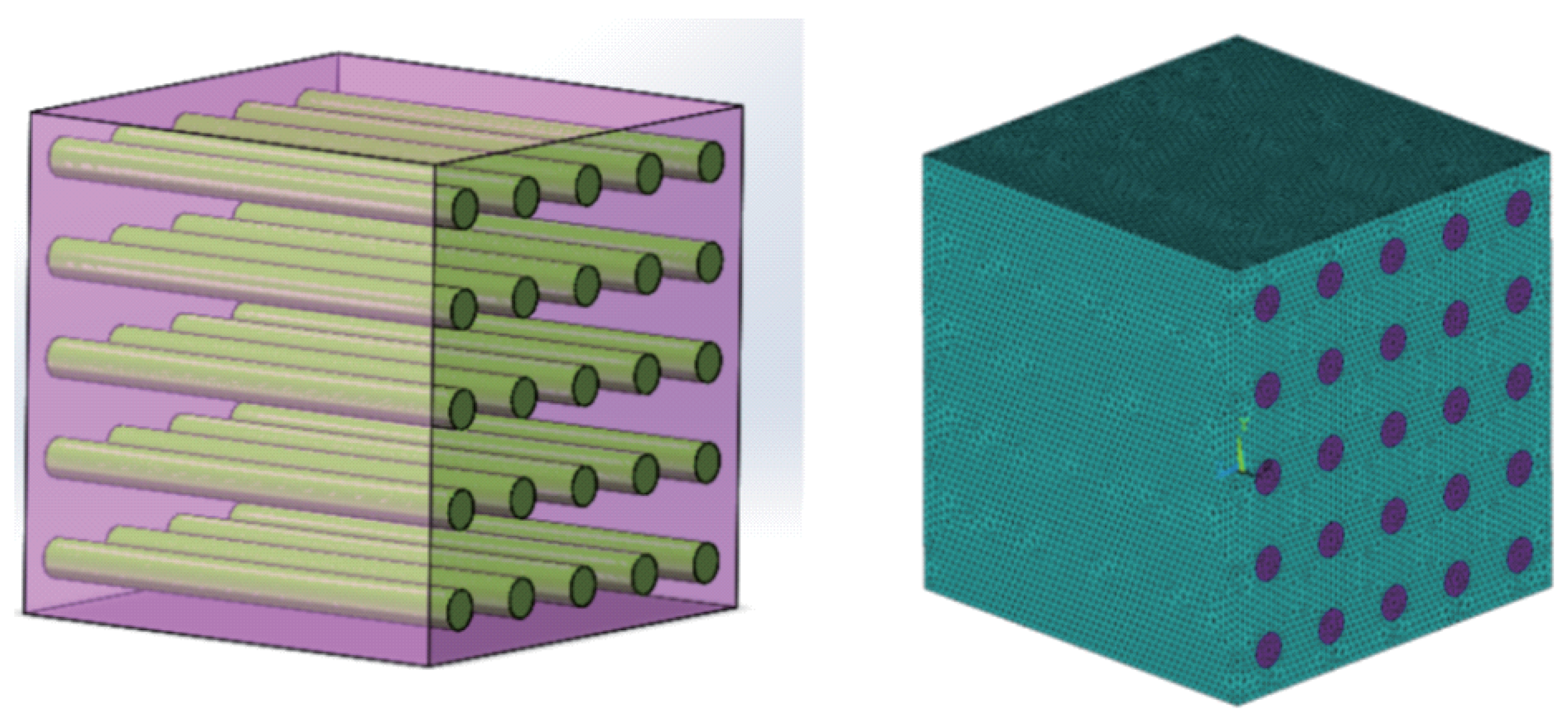
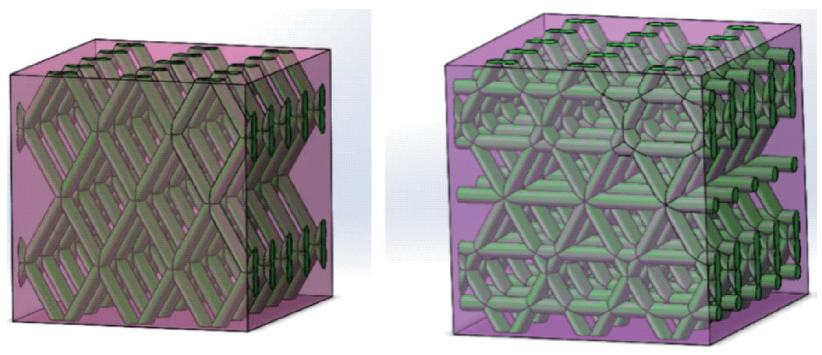
Through comparative analysis, the calculation results of explicit expression (64) were consistent with those of the FEM numerical simulations.

(6)

The Voigt model and the Reuss model only included the effect of the volume fraction. Both the Voigt model and the Reuss model cannot reflect the effect of the fiber direction distribution. As the fibers and the matrix in the three example were isotropic here, the effective elasticity tensors (80) and (83) of both the Voigt model and the Reuss model were isotropic. However, the effective elasticity tensors of the FEM simulation and the self-consistent method based on the eigenstrain were anisotropic.

(7)

We used the numerical simulation of FEM to check a constitutive model. The results of the self-consistent method based on the eigenstrain in Equation (74) were almost the same as those of FEM simulation in (87).

References

1. Zhang, H.; Sfarra, S.; Sarasini, F.; Santulli, C.; Fernandes, H.; Avdelidis, N.P.; Ibarra-Castanedo, C.; Maldague, X.P.V. Thermographic non-destructive evaluation for natural fiber-reinforced composite laminates. Appl. Sci. 2018, 8, 240. [Google Scholar] [CrossRef] [Green Version]
2. Vijay Kumar, V.; Ramakrishna, S.; Kong Yoong, J.L.; Esmaeely Neisiany, R.; Surendran, S.; Balaganesan, G. Electrospun nanofiber interleaving in fiber reinforced composites—Recent trends. Mater. Des. Process. Commun. 2019, 1, e24. [Google Scholar] [CrossRef] [Green Version]
3. Kerni, L.; Singh, S.; Patnaik, A.; Kumar, N. A review on natural fiber reinforced composites. Mater. Today Proc. 2020, 28, 1616–1621. [Google Scholar] [CrossRef]
4. Azman, M.A.; Asyraf, M.R.M.; Khalina, A.; Petrů, M.; Ruzaidi, C.M.; Sapuan, S.M.; Wan Nik, W.B.; Ishak, M.R.; IIyas, R.A.; Suriani, M.J. Natural fiber reinforced composite material for product design: A short review. Polymers 2021, 13, 1917. [Google Scholar] [CrossRef] [PubMed]
5. Talreja, R.; Waas, A.M. Concepts and definitions related to mechanical behavior of fiber reinforced composite materials. Compos. Sci. Technol. 2022, 217, 109081. [Google Scholar] [CrossRef]
6. Yang, G.; Park, M.; Park, S.J. Recent progresses of fabrication and characterization of fibers-reinforced composites: A review. Compos. Commun. 2019, 14, 34–42. [Google Scholar] [CrossRef]
7. Greco, F.; Leonetti, L.; Lonetti, P.; Luciano, R.; Pranno, A. A multiscale analysis of instability-induced failure mechanisms in fiber-reinforced composite structures via alternative modeling approaches. Compos. Struct. 2020, 251, 112529. [Google Scholar] [CrossRef]
8. Akbaş, Ş.D.; Ersoy, H.; Akgöz, B.; Civalek, Ö. Dynamic analysis of a fiber-reinforced composite beam under a moving load by the Ritz method. Mathematics 2021, 9, 1048. [Google Scholar] [CrossRef]
9. Bunge, H.J. Texture Analysis in Material Science: Mathematical Methods; Butterworths: London, UK, 1982. [Google Scholar]
10. Roe, R.J. Description of crystallite orientation in polycrystalline materials. III. General solution to pole figure inversion. J. Appl. Phys. 1965, 36, 2024–2031. [Google Scholar] [CrossRef]
11. Roe, R.J. Inversion of pole figures for materials having cubic crystal symmetry. J. Appl. Phys. 1966, 37, 2069–2072. [Google Scholar] [CrossRef]
12. Biedenharn, L.C.; Louck, J.D. Angular Momentum in Quantum Physics; Cambridge University Press: Cambridge, UK, 1984. [Google Scholar]
13. Varshalovich, D.A.; Moskalev, A.N.; Khersonskii, V.K. Quantum Theory of Angular Momentum; Word Scientific: Singapore, 1988. [Google Scholar]
14. Morris, P.R. Averaging fourth-rank tensors with weight functions. J. Appl. Phys. 1969, 40, 447–448. [Google Scholar] [CrossRef]
15. Sayers, C.M. Ultrasonic velocities in anisotropic polycrystalline aggregates. J. Phys. Appl. Phys. 1982, 15, 2157–2167. [Google Scholar] [CrossRef]
16. Voigt, W. Uber die beziehungzwischen den beiden elastizitäts konstanten isotroper korper. Wied. Ann. 1889, 38, 573–587. [Google Scholar] [CrossRef] [Green Version]
17. Reuss, A. Berchung der fiessgrenze von mischkristallen auf grund der plastizitätsbedingung für einkristalle. ZAMM-J. Appl. Math. Mech. Für Angew. Math. Und Mech. 1929, 9, 49–58. [Google Scholar] [CrossRef]
18. Kröner, E. Kontinuumstheorie der Versetzungen und Eigenspannungen; Springer: Berlin/Heidelberg, Germany, 1958. [Google Scholar]
19. Kröner, E. Zur plastischen verformung des vielkristalls. Acta Metall. 1961, 9, 155–161. [Google Scholar] [CrossRef]
20. Nemat-Nasser, S.; Hori, M. Micromechanics: Overall Properties of Heterogeneous Materials; Elsevier: Amsterdam, The Netherlands, 1993. [Google Scholar]
21. Morris, P.R. Elastic constants of polycrystals. Int. J. Eng. Sci. 1970, 8, 49–61. [Google Scholar] [CrossRef]
22. Huang, M. Elastic constants of a polycrystal with an orthorhombic texture. Mech. Mater. 2004, 36, 623–632. [Google Scholar] [CrossRef]
23. Huang, M. Perturbation approach to elastic constitutive relations of polycrystals. J. Mech. Phys. Solids 2004, 52, 1827–1853. [Google Scholar] [CrossRef]
24. Huang, M.; Man, C.S. A generalized Hosford yield function for weakly-textured sheets of cubic metals. Int. J. Plast. 2013, 41, 97–123. [Google Scholar] [CrossRef]
25. Dong, X.N.; Zhang, X.; Huang, Y.Y.; Guo, X.E. A generalized self-consistent estimate for the effective elastic moduli of fiber-reinforced composite materials with multiple transversely isotropic inclusions. Int. J. Mech. Sci. 2005, 47, 922–940. [Google Scholar] [CrossRef]
26. Mohankumar, D.; Rajeshkumar, L.; Muthukumaran, N.; Ramesh, M.; Aravinth, P.; Anith, R.; Balaji, S.V. Effect of fiber orientation on tribological behaviour of Typha angustifolia natural fiber reinforced composites. Mater. Today Proc. 2022, 62, 1958–1964. [Google Scholar] [CrossRef]
27. Hashin, Z.; Rosen, B.W. The elastic moduli of fiber-reinforced materials. J. Appl. Mech. 1964, 31, 223–232. [Google Scholar] [CrossRef]
28. Hashin, Z. On elastic behavior of fiber reinforced materials of arbitrary transverse phase geometry. J. Mech. Phys. Solids 1965, 13, 119–134. [Google Scholar] [CrossRef]
29. Hill, R. Theory of mechanical properties of fibre-strengthened materials-I elastic behavior. J. Mech. Phys. Solids 1964, 12, 199–212. [Google Scholar] [CrossRef]
30. Hill, R. Theory of mechanical properties of fibre-strengthened materials-III self-consistent model. J. Mech. Phys. Solids 1965, 13, 189–198. [Google Scholar] [CrossRef]
31. Tian, L.; Zhao, H.; Yuan, M.; Wang, G.; Zhang, B.; Chen, J. Global buckling and multiscale responses of fiber-reinforced composite cylindrical shells with trapezoidal corrugated cores. Compos. Struct. 2021, 260, 113270. [Google Scholar] [CrossRef]
32. Man, C.S.; Huang, M. A representation theorem for material tensors of weakly-textured polycrystals and its applications in elasticity. J. Elast. 2012, 106, 1–42. [Google Scholar] [CrossRef]
33. Mura, T. Micromechanics of Defects in Solids; Martinus Nijhoff Publishers: Leiden, The Netherlands, 1982. [Google Scholar]
34. Eshelby, J.D. The determination of the elastic field of an ellipsoidal inclusion, and related problems. Proc. R. Soc. Lond. Ser. A Math. Phys. Sci. 1957, 241, 376–396. [Google Scholar]
35. Mori, T.; Tanaka, K. Average stress in matrix and average elastic energy of materials with misfitting inclusions. Acta Metall. 1973, 21, 571–574. [Google Scholar] [CrossRef]
36. Liu, L.; Huang, Z. A note on Mori-Tanaka’s method. Acta Mech. Solida Sinica 2014, 27, 234–244. [Google Scholar] [CrossRef]
37. Benveniste, Y. A new approach to the application of Mori-Tanaka’s theory in composite materials. Mech. Mater. 1987, 6, 147–157. [Google Scholar] [CrossRef]
38. Huang, M.; Man, C.S. A finite-element study on constitutive relation HM-V for elastic polycrystals. Comput. Mater. Sci. 2005, 32, 378–386. [Google Scholar] [CrossRef]
Figure 1. Fiber-reinforced orthorhombic composite material Ω , Cartesian coordinate system x i and fiber direction ϕ p .
Crystals 12 01004 g001
Figure 2. Fiber-reinforced orthorhombic composite material Ω for example 1 and its FEM model.
Crystals 12 01004 g002
Figure 3. Fiber-reinforced orthorhombic composite materials for example 2 (left) and example 3 (right).
Crystals 12 01004 g003
Publisher’s Note: MDPI stays neutral with regard to jurisdictional claims in published maps and institutional affiliations.