Molecular–Statistical Theory for the Description of Re-Entrant Ferroelectric Phase

Abstract

The re-entrant ferroelectric phase (Sm-$C_{\mathrm{re}}^{*}$) is investigated in the framework of a molecular–statistical approach. It was found that anticlinic synpolar along the smectic layer normal phase can arise below the antiferroelectric phase (Sm-$C_A^{*}$) in the temperature scale, and we suggest this phase to be Sm-$C_{\mathrm{re}}^{*}$. We have shown that in the vicinity of Sm-$C_A^{*}$–Sm-$C_{\mathrm{re}}^{*}$ phase transition temperature, a very small electric field can cause a transition into the bidomain synclinic phase, where the helical pitch is unwound and the tilt planes have contributions either along or against the electric field. The helical rotation, elasticity and deformation of the Sm-$C^{*}$, Sm-$C_A^{*}$ and Sm-$C_{\mathrm{re}}^{*}$ structures without electric field or in the presence of electric field, as well as the dielectric response, are investigated. It is shown that Sm-$C_{\mathrm{re}}^{*}$ can arise solely due to the dipole–dipole interaction, and thus, in contrast to the conventional (improper) ferroelectric Sm-$C^{*}$, appears to be the proper ferroelectric phase.

1. Introduction

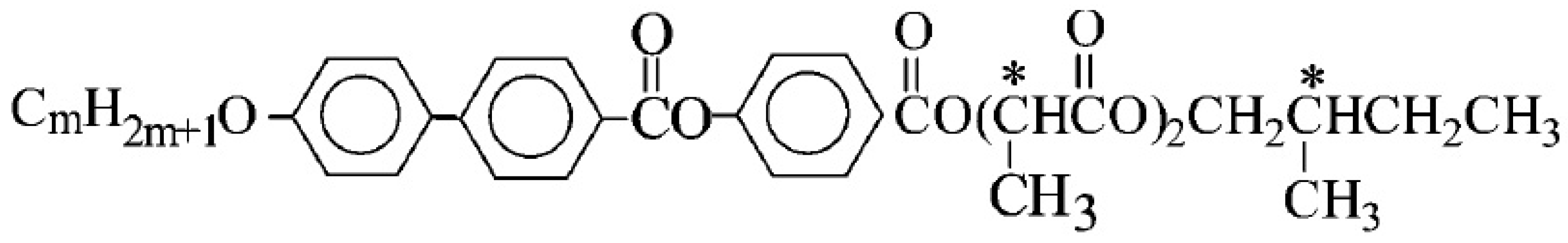
Ferroelectricity in smectic liquid crystals was discovered by Meyer [1]. Antiferroelectric smectic phases were discovered later in [2]. The LC lactic acid derivatives are the unique ferroelectric materials. In particular, they can form the antiferroelectric, hexatic, Sm-X [3,4] and various kinds of re-entrant phases [5]. They also can be used for the synthesis of the side chain polysiloxanes, which are the well-aligned polar polymers [6]. In the majority of antiferroelectric materials, the antiferroelectric Sm-$C_A^{*}$ phase is observed at lower temperature than the ferroelectric Sm-$C^{*}$ smectic phase. However, in lactic acid derivative ZLL $7{/}^{*}$, the ferroelectric phase reappears below the antiferroelectric phase in the temperature scale [5]. The general molecular formulae for ZLL $m{/}^{*}$ materials is presented in Figure 1. A ZLL $m{/}^{*}$ molecule consists of a rigid core and two flexible tails. It is remarkable that one of the molecular tails contains several transverse dipole moments, each one in the vicinity of a chiral center (marked with stars in Figure 1). The series of ferroelectric liquid crystals with several chiral centers in the molecular tail were investigated in Ref. [7], where in particular, it was reported about the existence of the Sm-$C_{\mathrm{re}}^{*}$ phase in ZLL $7{/}^{*}$ material. Another tail of a molecule is also quite long. The re-entrant ferroelectric phase also tends to appear in the mixtures of the ZLL $6{/}^{*}$ and ZLL $8{/}^{*}$ lactic acids [5], and thus, seven chains in the long molecular tail appear to be optimal for the emergence of the re-entrant ferroelectric phase.

The existence of the Sm-$C_{\mathrm{re}}^{*}$ phase was confirmed by various experimental data, for example, by birefringence [8], calorimetry [3], nuclear magnetic resonance and dielectric spectroscopy [9,10,11] measurements. In the electric field–temperature phase diagram the antiferroelectric smectic phase appears to be isolated, in other words, is surrounded by the ferroelectric smectic phase [8]. It was also noticed that the ferroelectric phase consists of several anomaly regions. The origin of re-entrant ferroelectric phase should be related to polarization effects. Theory predicts the three kinds of polarization in each smectic layer i [12,13,14,15]:

$$\begin{array}{c}\hfill c_f[{\mathbf{n}}_i\times [\Delta {\mathbf{n}}_{i\pm 1}\times {\mathbf{n}}_i]+c_p({\mathbf{n}}_i·{\mathbf{k}}_0)[{\mathbf{n}}_i·{\mathbf{k}}_0]-\frac{1}{4}\beta \mu [{\mathbf{n}}_i\times [\mathbf{E}\times {\mathbf{n}}_i]],\end{array}$$

(1)

where the first two terms, flexoelectric and piezoelectric ones, arise spontaneously, while the third term is induced polarization due to reorientation of permanent molecular dipoles in the electric filed. One notes that for example, piezoelectric polarization in Sm-$C^{*}$ and Sm-$C_A^{*}$ [the second term in Equation (1)] favors the orientation of tilt planes perpendicular to the electric field, while anisotropy of coupling of induced polarizations in the neighboring smectic layers [the third term in Equation (1)] favors longitudinal to the electric field orientation of tilt planes.

If polarization is small, it is possible to obtain the set of simple equations for polarization in each smectic layer i [12,13,14,15]:

$${\mathbf{P}}_i+\widehat{\mathbf{g}}[{\mathbf{P}}_{i-1}+{\mathbf{P}}_{i+1}]=-\rho \mu \widehat{\chi }{\mathbf{M}}_i,$$

(2)

containing the coupling tensor $\widehat{\mathbf{g}}$ between polarizations in the neighboring layers, which originates from the dipole–dipole interaction of molecules located in the neighboring smectic layers [12,13,14,15]:

$$\begin{array}{c}\hfill \widehat{\mathbf{g}}\approx \left[\begin{array}{ccc}{g}_1& 0& 0\\ 0& g_1& 0\\ 0& 0& -2g_1\end{array}\right],\end{array}$$

(3)

where the $xx$, $yy$ and $zz$ components of tensor are the average interactions between the projections of molecular dipoles on the corresponding axes. The local molecular field ${\mathbf{M}}_i$ in Equation (2) contains, in particular, the piezoelectric and flexoelectric terms and the interaction of molecular dipoles with higher multipoles and with the electric field. In the synclinic phase (where polarization is the same in each smectic layer) from Equation (2) it follows:

$${\mathbf{P}}_i=-\rho \mu \widehat{\omega }{\mathbf{M}}_i,$$

(4)

where the longitudinal and orthogonal to the smectic layer plane residual dielectric susceptibility can be written in the following form:

$${\omega }_{\Vert }=\frac{{\chi }_{\Vert }}{1+2g_1},{\omega }_{\perp }=\frac{{\chi }_{\perp }}{1-4g_1}.$$

(5)

In correspondence with Equation (5), the residual spontaneous polarization along the smectic layer plane is diminished with respect to that of an isolated single smectic layer because of the unfavorable side-by-side coupling of dipoles in the neighboring layers. On the contrary, polarization along the smectic layer normal is enhanced because of the favorable head-and-tail coupling of the same dipoles, generally with projections as on the smectic layer plane, as on the smectic layer normal, in the tilted smectic phase. It is known that the coupling parameter $g_1$ increases with the increasing tilt angle $\theta$ [12,13,14,15]:

$$g_1\sim \frac{{\mathbf{\mu }}_{ef}^2}{{cos}^3\theta }$$

(6)

where ${\mu }_{ef}\equiv \mu /\sqrt{k_B{T}^{*}{d}^3}$ is the effective molecular dipole of the molecular tail, where $\mu$ is the electric dipole itself, $k_B$ is the Boltzmann constant, d is the molecular breadth and $T^{*}$ is the temperature of transition into the orthogonal Sm-$A*$ phase, while the tilt angle $\theta$ increases with the decreasing temperature in Sm-$C^{*}$ and/or Sm-$C_A^{*}$ phases below this temperature.

Formally, from Equation (2) it follows that ${\omega }_{\perp }$ becomes infinitely large when $g_1$ reaches $1/4$. In most of smectic materials this situation does not happen, which means that the coupling parameter $g_1$ [see Equation (6)] does not reach considerably large values when the tilt angle $\theta$ increases with the decreasing temperature. At the same time, if we suppose that the molecular flexible tails are very long and contain several transverse dipole moments attached to their own chiral centers, in particular, far from the molecular core, we can imagine that some of them can be oriented along the smectic layer normal. At the same time, since they are connected with the molecular core, all tendencies related to their azimuthal orientation can be translated into the molecular core. The infinitely large ${\omega }_{\perp }$ says presumably about the induction of the normal to the smectic layer surfaces spontaneous polarization below the temperature corresponding to $g_1=1/4$. It is impossible to investigate the structure below this temperature in the framework of linear approximation for polarization, and the more general approach is needed.

In the present paper, we are going to consider the Maier–Saupe theory for polarization (polar order parameter), when the distribution function for the orientation of transverse molecular dipoles is determined by the molecular mean field and by the external electric field. It will be demonstrated that the proper ferroelectric phase (in contrast to the improper conventional ferroelectric Sm-$C^{*}$ phase) can arise at lower temperature if the molecular tails are sufficiently disordered (and thus, are sufficiently long). In other words, the dipole–dipole interaction itself can promote the existence of ferroelectric phase. One can imagine, for example, the disc-like molecules with the dipoles perpendicular to their main planes. In the case of disc-like molecules, the dipoles would prefer to be oriented parallel to each other in the “head-and-tail” configuration. In our case, the molecules are elongated, and, at the first glance, nothing should promote the proper ferroelectricity. However, the molecules of lactic acids have very long flexible tails with several transverse dipoles. The rigid molecular cores also possess the transverse dipole moments. If we propose that the molecular tails are flexible only in prime direction (along the chain), but the secondary axes of each link can only rotate all together (in the same manner as in the jump rope), it is easy to realize that the azimuthal orientations of all the dipoles along the chain of a flexible tail will be strongly correlated with each other. In particular, the rotation of a dipole located in the rigid molecular core around the long molecular axis will cause the rotation of all dipoles located in the molecular tail by the same angle around their local chain directions. One notes, however, that in the long molecular tails, which are flexible in prime direction, some dipoles can point perpendicular to the smectic layer, and thus, contribute to the “head-and-tail” dipole–dipole interaction in the neighboring smectic layers. Their azimuthal orientation will automatically be transmitted into the molecular core, and thus, the dipole–dipole interaction of dipoles located in the molecular tails will result in the appearance of proper polarization due to the induced in this way particular orientation of transverse dipoles located in the molecular cores.

2. Molecular Model

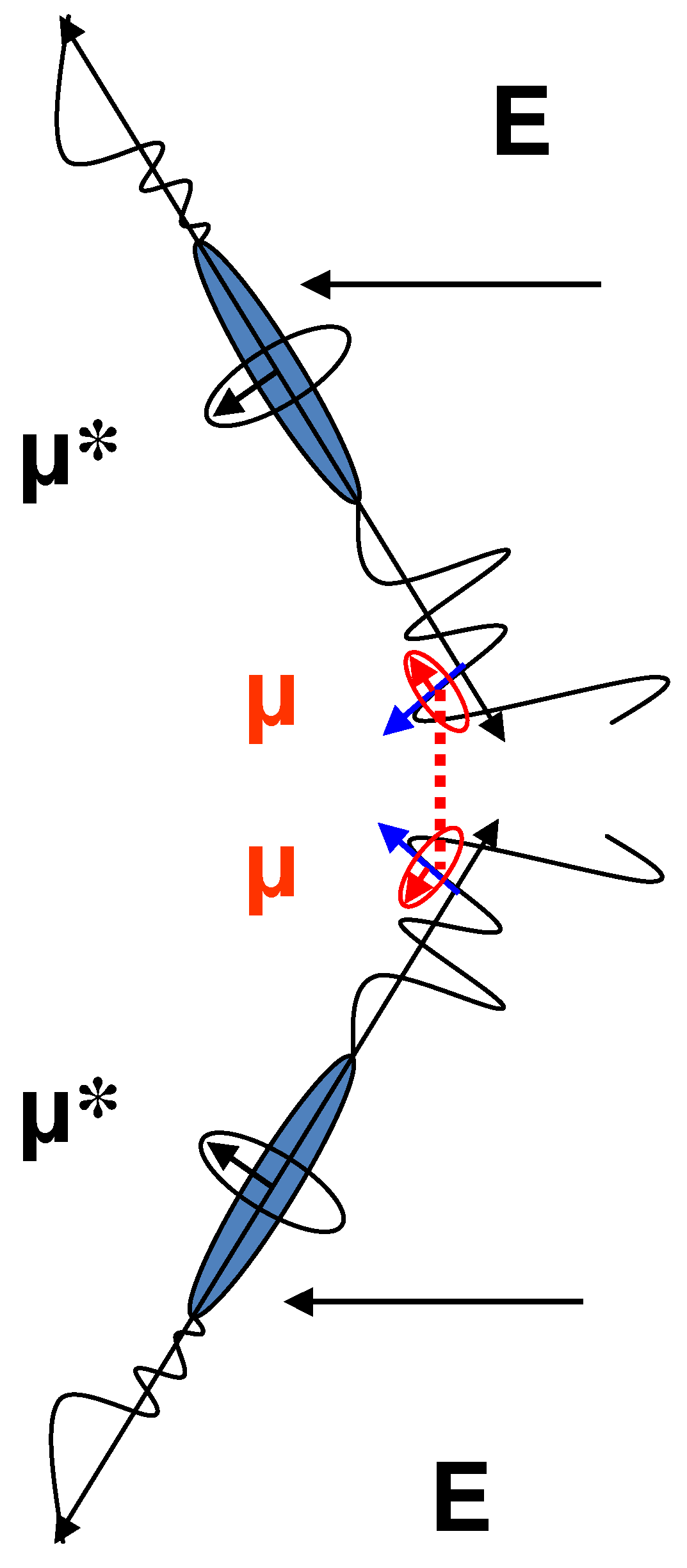
Let us consider the smectic structure, where molecules consist of the rigid cores and flexible tails (Figure 2).

The molecular tails in each smectic layer i can possess the nematic order with director ${\mathbf{n}}_i$ coinciding for simplicity with principal orientation of the rigid molecular cores in the same layer. Orientation of director ${\mathbf{n}}_i$ is specified by tilt angle $\theta$ assumed to be the same in every layer, and by azimuthal angle ${\phi }_i$, which can vary from layer to layer. We expect that real molecule can possess several dipole moments as in the core, as in the tail. Let us consider a simple model, where each molecule possesses one large transverse dipole moment ${\mathbf{\mu }}^{*}$ in the core and one small transverse dipole moment $\mathbf{\mu }$ in the tail. Let us consider a jump rope model for a molecular tail. Suppose that molecular tails are flexible in prime axis orientation, but, at the same time, are rigid in the biaxial orientation, so that rotation of dipole $\mathbf{\mu }$ located in tail by angle $\psi$ around local $\mathbf{a}$-axis in the tail causes rotation of dipole ${\mathbf{\mu }}^{*}$ located in the rigid core by the same angle $\psi$ around director $\mathbf{n}$. Change over from laboratory frame $\{\mathbf{x},\mathbf{y},\mathbf{z}\}$ to local frame $\{{\mathbf{w}}_i,{\mathbf{m}}_i^{\prime },\mathbf{n}\}$ related to the molecular core in layer i requires the rotation by angle ${\phi }_i$ around $\mathbf{z}$-axis and then rotation by angle $\theta$ around new ${\mathbf{w}}_i$-axis. Dipole moment ${\mathbf{\mu }}_i^{*}$ belongs to the plane of axes ${\mathbf{w}}_i$ and ${\mathbf{m}}_i^{\prime }$. Farther change over from frame $\{{\mathbf{w}}_i,{\mathbf{m}}_i^{\prime },\mathbf{n}\}$ to local frame $\{{\mathbf{b}}_i,{\mathbf{c}}_i,{\mathbf{n}}_i\}$ related to the molecular tail in layer i requires the rotation by angle ${\phi }_i^{\prime }$ around $\mathbf{n}$-axis and then rotation by angle ${\theta }^{\prime }$ around new ${\mathbf{b}}_i$-axis. Dipole moment ${\mathbf{\mu }}_i$ belongs to the plane of axes ${\mathbf{b}}_i$ and ${\mathbf{c}}_i$. Since the plane of axes ${\mathbf{w}}_i$ and ${\mathbf{m}}_i^{\prime }$ is parallel to the plane of axes ${\mathbf{w}}_i$ and ${\mathbf{b}}_i$, it is convenient to change over from angle $\psi$ to angle $\psi -{\phi }^{\prime }$, i.e., to count orientation of both dipoles ${\mathbf{\mu }}_i$ and ${\mathbf{\mu }}_i^{*}$ from the same ${\mathbf{b}}_i$-axis. In the model of jump rope angles $\psi -{\phi }^{\prime }$ and ${\psi }^{\prime }$ appear to be equal. In the following consideration we will omit the apostrophe and use definition $\psi$ for both angles.

It was shown in [16,17] that dipoles $\mathbf{\mu }$ belonging to the neighboring smectic layers should have positional correlation, because they are located near the border between layers (see Figure 3).

At the same time, we do not expect that dipoles ${\mathbf{\mu }}^{*}$ located far from the border between layers have positional correlations either with each other in the neighboring layers, or even with dipoles $\mathbf{\mu }$ within the same layers. Dipoles located in the molecular cores are expected to be essentially larger than dipoles located in tails, and in this case only interaction of dipoles ${\mathbf{\mu }}^{*}$ with external electric field $\mathbf{E}$ can be taken into account and only piezoelectric effect related to dipoles ${\mathbf{\mu }}^{*}$ can be considered. However, the distance between terminal dipoles $\mathbf{\mu }$ is essentially smaller than distance between dipoles ${\mathbf{\mu }}^{*}$ located in cores. In this case, only interaction between dipoles $\mathbf{\mu }$ in neighboring smectic layers can be taken into account. If the flexible tails possess low nematic order, the interacting dipoles $\mathbf{\mu }$ can be almost freely oriented in the space, while their azimuthal part of orientation is translated to the molecular cores and influences the azimuthal orientation of dipoles ${\mathbf{\mu }}^{*}$ located in molecular cores, which on the other hand, should influence the orientation of director $\mathbf{n}$ in the electric field.

3. Free Energy of Smectic Molecules with Transverse Dipoles in Rigid Cores and in Flexible Tails

One should generalize the distribution function considered in [12,16,17] to take into account orientations of tails and orientations of dipoles $\mathbf{\mu }$ and ${\mathbf{\mu }}^{*}$ around axes $\mathbf{a}$ and $\mathbf{n}$, respectively. In the framework of this approach there should be two types of the order parameters: (1) nematic order parameters for the principal orientations of tails and (2) polarization. It is clear that nematic ordering of tails is determined by their anisotropic interactions with mostly different origin than polarization. Therefore, let us simply consider the nematic order parameters as input parameters, and let us determine the polarization. A part of the free energy of tilted smectic state explicitly depending on the distribution function $f\left(\right(\mathbf{a}·\mathbf{n}),\psi )$ can be written in the following way (compare to [12,17]):

$$\begin{array}{cc}\frac{F}{\rho k_{B}T}\hfill & =\sum _i\int d^2{\mathbf{a}}_{1}d{\psi }_{1}f(({\mathbf{a}}_1·{\mathbf{n}}_i),{\psi }_1)lnf(({\mathbf{a}}_1·{\mathbf{n}}_i),{\psi }_1)\hfill \\ \hfill & +\frac{1}{2}\sum _{i,j}\int d^2{\mathbf{a}}_{1}d{\psi }_1{d}^2{\mathbf{a}}_{2}d{\psi }_{2}f(({\mathbf{a}}_1·{\mathbf{n}}_i),{\psi }_1)\hfill \\ \hfill & \times f(({\mathbf{a}}_2·{\mathbf{n}}_j),{\psi }_2)\{u_0({\mathbf{a}}_1,{\mathbf{a}}_2)-{\mathbf{\mu }}_i({\mathbf{a}}_1,{\psi }_1){\widehat{\mathbf{g}}}_{|j-i|}{\mathbf{\mu }}_j({\mathbf{a}}_2,{\psi }_2)\}\hfill \\ \hfill & -{\mathbf{M}}_i\sum _i\int d^2{\mathbf{a}}_{1}d{\psi }_1{f}_i(({\mathbf{a}}_1·{\mathbf{n}}_i),{\psi }_1){\mathbf{\mu }}_i^{*}\left({\psi }_1\right),\hfill \end{array}$$

(7)

where the first term is the orientational entropy, the second term is the averaged with respect to translational coordinates interaction between a fragment of flexible tail of molecule 1 located in layer i containing dipole moment ${\mathbf{\mu }}_i$ and a fragment of flexible tail of molecule 2 located in layer j containing dipole moment ${\mathbf{\mu }}_j$, while the third term describes an influence of the local field ${\mathbf{M}}_i$ on the transverse dipole moment ${\mathbf{\mu }}_i^{*}$ in the rigid core of a molecule located in layer i. Orientation of prime axes ${\mathbf{a}}_1$ and ${\mathbf{a}}_2$ of fragments mentioned above is determined mostly by their dispersion interaction $u_0({\mathbf{a}}_1,{\mathbf{a}}_2)$ which is assumed to be independent of the orientation of dipoles ${\mathbf{\mu }}_i$ and ${\mathbf{\mu }}_j$, while orientation of dipoles themselves around prime axes is determined by dipole–dipole interaction $-{\mathbf{\mu }}_i({\mathbf{a}}_1,{\psi }_1){\widehat{\mathbf{g}}}_{|j-i|}{\mathbf{\mu }}_j({\mathbf{a}}_2,{\psi }_2)$. In the model of a jump rope, the azimuthal orientation of dipole moment ${\mathbf{\mu }}_i^{*}$ located in the rigid core around ${\mathbf{n}}_i$ is biased to the azimuthal orientation of dipole moment ${\mathbf{\mu }}_i$ located in the molecular tail around ${\mathbf{a}}_1$ (for simplicity, both orientations are described by the same azimuthal angle ${\psi }_1$). For convenience we consider both dipoles $\mathbf{\mu }$ and ${\mathbf{\mu }}^{*}$ in each layer as dimensionless vectors, while the dimension of dipole $\mathbf{\mu }$ is included into the dipolar coupling tensors [17]

$$\begin{array}{c}{\left({\widehat{\mathbf{g}}}_0\right)}_{\alpha \beta }\equiv \frac{1}{4}{\mu }_{\mathrm{ef}}^2\left[{\widehat{\mathbf{\delta }}}_{\alpha \beta }\left(1-\frac{3}{2}{\theta }^2\right)+\frac{3}{2}{\theta }^2{\left({\mathbf{w}}_i\right)}_{\alpha }{\left({\mathbf{w}}_i\right)}_{\beta }\right],\hfill \\ {\left({\widehat{\mathbf{g}}}_1\right)}_{\alpha \beta }\equiv -\frac{{\mu }_{\mathrm{ef}}^2}{2{cos}^3\theta }({\widehat{\mathbf{\delta }}}_{\alpha \beta }-3{\mathbf{k}}_{\alpha }{\mathbf{k}}_{\beta }),\hfill \end{array}$$

(8)

where ${\mu }_{\mathrm{ef}}\equiv \mu /{\left(k_{B}T{d}^3\right)}^{1/2}$, d is the molecular breadth, $\theta$ is the tilt angle, ${\mathbf{w}}_i$ is the unit vector perpendicular to the tilt plane in layer i (see Figure 2), $\mathbf{k}$ is the smectic layer normal, and dimension of dipole ${\mathbf{\mu }}^{*}$ is included into the local field [12]

$$\begin{array}{c}\hfill {\mathbf{M}}_i\equiv c_p({\mathbf{n}}_i·\mathbf{k})[{\mathbf{n}}_i\times \mathbf{k}]+c_f[{\mathbf{n}}_i\times [\Delta {\mathbf{n}}_{i\pm 1}\times {\mathbf{n}}_i]]+\frac{{\mu }^{*}}{k_{B}T}[{\mathbf{n}}_i\times [\mathbf{E}\times {\mathbf{n}}_i]]\end{array}$$

(9)

where $\mathbf{E}$ is the external electric field, ${\mathbf{n}}_i$ is the nematic director in layer i, and parameters $c_p$ and $c_f$ are the piezoelectric and flexoelectric constants, respectively. In Equation (9) we have taken into account in advance only projection of the local field ${\mathbf{M}}_i$ on the plane, which is perpendicular to director ${\mathbf{n}}_i$, because only this projection survives after multiplication by the transverse dipole moment ${\mathbf{\mu }}^{*}$ in Equation (7) for the free energy. Taking into account interaction between terminal dipoles within the same and in the neighboring smectic layers only and minimizing free energy (7) with respect to the orientational distribution function $f_i\equiv f(({\mathbf{a}}_1·{\mathbf{n}}_i),{\psi }_1)$, one obtains:

$$f_i=\frac{f_0}{Z_i}exp\{{\mathbf{\mu }}_i[{\widehat{\mathbf{g}}}_0{\mathbf{p}}_i+{\widehat{\mathbf{g}}}_1({\mathbf{p}}_{i-1}+{\mathbf{p}}_{i+1})]+{\mathbf{\mu }}_i^{*}{\mathbf{M}}_i\},$$

(10)

where $f_0=f_0({\mathbf{a}}_1·\mathbf{n})$ is the orientational distribution function for the prime axes of flexible tails depending mostly on their dispersion interaction $u_0({\mathbf{a}}_1,{\mathbf{a}}_2)$,

$$\begin{array}{c}\hfill Z_i=\int d^2{\mathbf{a}}_{1}d{\psi }_1{f}_{0}exp\{{\mathbf{\mu }}_i[{\widehat{\mathbf{g}}}_0{\mathbf{p}}_i+{\widehat{\mathbf{g}}}_1({\mathbf{p}}_{i-1}+{\mathbf{p}}_{i+1})]+{\mathbf{\mu }}_i^{*}{\mathbf{M}}_i\},\end{array}$$

(11)

where ${\mathbf{p}}_i$ is the average dimensionless dipole moment ${\mathbf{\mu }}_i$:

$$\begin{array}{c}\hfill {\mathbf{p}}_i=\frac{1}{Z_i}\int d^2{\mathbf{a}}_{1}d{\psi }_1{f}_0{\mathbf{\mu }}_{i}exp\{{\mathbf{\mu }}_i[{\widehat{\mathbf{g}}}_0{\mathbf{p}}_i+{\widehat{\mathbf{g}}}_1({\mathbf{p}}_{i-1}+{\mathbf{p}}_{i+1})]+{\mathbf{\mu }}_i^{*}{\mathbf{M}}_i\}.\end{array}$$

(12)

By analogy one obtains the following expression for the average dimensionless dipole moment ${\mathbf{\mu }}_i^{*}$

$$\begin{array}{c}\hfill {\mathbf{p}}_i^{*}=\frac{1}{Z_i}\int d^2{\mathbf{a}}_{1}d{\psi }_1{f}_0{\mathbf{\mu }}_i^{*}exp\{{\mathbf{\mu }}_i[{\widehat{\mathbf{g}}}_0{\mathbf{p}}_i+{\widehat{\mathbf{g}}}_1({\mathbf{p}}_{i-1}+{\mathbf{p}}_{i+1})]+{\mathbf{\mu }}_i^{*}{\mathbf{M}}_i\}.\end{array}$$

(13)

Equations (11) and (12) are the recurrent equations for determination of polarization ${\mathbf{p}}_i$ in each smectic layer i, from where polarization ${\mathbf{p}}_i^{*}$ can be calculated according to Equations (11) and (13).

4. Spontaneous Polarization in the Absence of Piezoelectricity and Flexoelectricity

Let us consider the right-handed local coordinate system as shown in Figure 2 with ${\mathbf{w}}_i$-axis perpendicular to the local tilt plane in layer i, ${\mathbf{m}}_i$-axis parallel to the local tilt direction in layer i within the smectic layer plane, and $\mathbf{k}$-axis parallel to the smectic layer normal. Usually polarization is called spontaneous if it arises at $E=0$. Typically, it arises due to the presence of piezoelectricity and/or flexoelectricity (i.e., due to the first two terms in Equation (9) for local field ${\mathbf{M}}_i$). Both piezoelectric and flexoelectric terms are due to interactions of molecular dipole with higher multipoles. It is believed that spontaneous polarization cannot arise due to the dipole–dipole interaction itself. From Equations (11) and (12) it, however, follows that polarization can arise even at $\mathbf{M}=\mathbf{0}$. Indeed, Equations (11) and (12) are very similar to Maier–Saupe equations for determination of the orientational order parameter in nematics, if one considers dimensionless polarization ${\mathbf{p}}_i$ as vector order parameter, whose projections on the coordinate axes ${\mathbf{w}}_i$, ${\mathbf{m}}_i$ and $\mathbf{k}$ can vary from zero to one.

Thus, let us first consider the $\mathbf{M}=\mathbf{0}$ case, when dimensionless polarization ${\mathbf{p}}_0$ is expected to be the same in each smectic layer, if it is considered in the local coordinate system $\{{\mathbf{w}}_i,{\mathbf{m}}_i,\mathbf{k}\}$ of particular layer i. In the framework of perturbation theory, one can neglect a small influence of the helical rotation on polarization. In this approximation, in the anticlinic phase the local coordinate system exhibits rotation from layer to layer by angle $\pi$ around smectic layer normal $\mathbf{k}$, and therefore the longitudinal projections (parallel to the smectic layer plane) of polarizations ${\mathbf{p}}_{i-1}$ and ${\mathbf{p}}_{i+1}$ in the local coordinate system of layer i in Equations (10)–(12) should be taken with opposite sign to that in the local coordinate system of layers $i-1$ and $i+1$, while the normal projection (perpendicular to the smectic layer plane) should be taken with the same sign. Since both tensors ${\widehat{\mathbf{g}}}_0$ and ${\widehat{\mathbf{g}}}_1$ are diagonal in the local coordinate system of each layer, it is more convenient to introduce a new tensor ${\widehat{\mathbf{g}}}_1^A$ with opposite signs of components ${\left({\widehat{\mathbf{g}}}_1^A\right)}_{ww}$ and ${\left({\widehat{\mathbf{g}}}_1^A\right)}_{mm}$ to those of tensor ${\widehat{\mathbf{g}}}_1$, and the same sign of component ${\left({\widehat{\mathbf{g}}}_1^A\right)}_{kk}$ as that of tensor ${\widehat{\mathbf{g}}}_1$:

$${\left({\widehat{\mathbf{g}}}_1^A\right)}_{\alpha \beta }\equiv \frac{{\mu }_{\mathrm{ef}}^2}{2{cos}^3\theta }({\widehat{\mathbf{\delta }}}_{\alpha \beta }+{\mathbf{k}}_{\alpha }{\mathbf{k}}_{\beta }).$$

(14)

Let us also introduce the general tensors taking into account both couplings between polarizations within the same layers and in the neighboring layers: ${\widehat{\mathbf{g}}}^{\pm }\equiv {\widehat{\mathbf{g}}}_0\pm 2{\widehat{\mathbf{g}}}_1$ in the synclinic phase, or ${\widehat{\mathbf{g}}}^{\pm }\equiv {\widehat{\mathbf{g}}}_0\pm 2{\widehat{\mathbf{g}}}_1^A$ in the anticlinic phase. Taking into account this difference in definition, one obtains from Equations (11) and (12) similar types of equations for polarization in both synclinic and anticlinic phases:

$$\begin{array}{c}{\mathbf{p}}_0=\frac{1}{Z_0}\int d^2{\mathbf{a}}_{1}d{\psi }_1{f}_0{\mathbf{\mu }}_{i}exp\{{\mathbf{\mu }}_i{\widehat{\mathbf{g}}}^{+}{\mathbf{p}}_0\},\hfill \\ Z_0=\int d^2{\mathbf{a}}_{1}d{\psi }_1{f}_{0}exp\{{\mathbf{\mu }}_i{\widehat{\mathbf{g}}}^{+}{\mathbf{p}}_0\}.\hfill \end{array}$$

(15)

Expanding a combination of Equation (15) in Taylor series with respect to polarization ${\mathbf{p}}_0$ up to the third power and integrating as shown in Appendix A, one obtains the following equation for polarization:

$${\mathbf{p}}_0=\frac{1}{Z_0}\widehat{\mathbf{r}}{\mathbf{p}}_0,$$

(16)

where

$$\begin{array}{cc}{\widehat{\mathbf{r}}}_{\alpha \beta }\approx \hfill & \frac{1}{2}\left\{\left(\frac{2}{3}+\frac{1}{3}{S}_2\right){\widehat{\mathbf{g}}}_{\alpha \beta }^{+}-S_2{\mathbf{n}}_{\alpha }{\left({\widehat{\mathbf{g}}}^{+}\mathbf{n}\right)}_{\beta }\right\}\hfill \\ \hfill & +\frac{1}{16}\{\left(\frac{8}{15}+\frac{8}{21}{S}_2+\frac{3}{35}{S}_4\right){\mathbf{q}}_0^2{\widehat{\mathbf{g}}}_{\alpha \beta }^{+}\hfill \\ \hfill & -\left(\frac{4}{7}{S}_2+\frac{3}{7}{S}_4\right)[{\left(\mathbf{n}{\mathbf{q}}_0\right)}^2{\widehat{\mathbf{g}}}_{\alpha \beta }^{+}+{\mathbf{q}}_0^2{\mathbf{n}}_{\alpha }{\left({\widehat{\mathbf{g}}}^{+}\mathbf{n}\right)}_{\beta }]\hfill \\ \hfill & +S_4{\left(\mathbf{n}{\mathbf{q}}_0\right)}^2{\mathbf{n}}_{\alpha }{\left({\widehat{\mathbf{g}}}^{+}\mathbf{n}\right)}_{\beta }\},\hfill \end{array}$$

(17)

$$Z_0\approx 1+\frac{1}{4}\left[\left(\frac{2}{3}+\frac{1}{3}{S}_2\right){\mathbf{q}}_0^2-S_2{\left(\mathbf{n}{\mathbf{q}}_0\right)}^2\right],$$

(18)

where ${\mathbf{q}}_0\equiv {\widehat{\mathbf{g}}}^{+}{\mathbf{p}}_0$, and the nematic order parameters for prime axes of flexible molecular tails are given by the following equation:

$$S_i\equiv \int d^2\mathbf{a}{f}_0(\mathbf{a}·\mathbf{n})P_i(\mathbf{a}·\mathbf{n}),$$

(19)

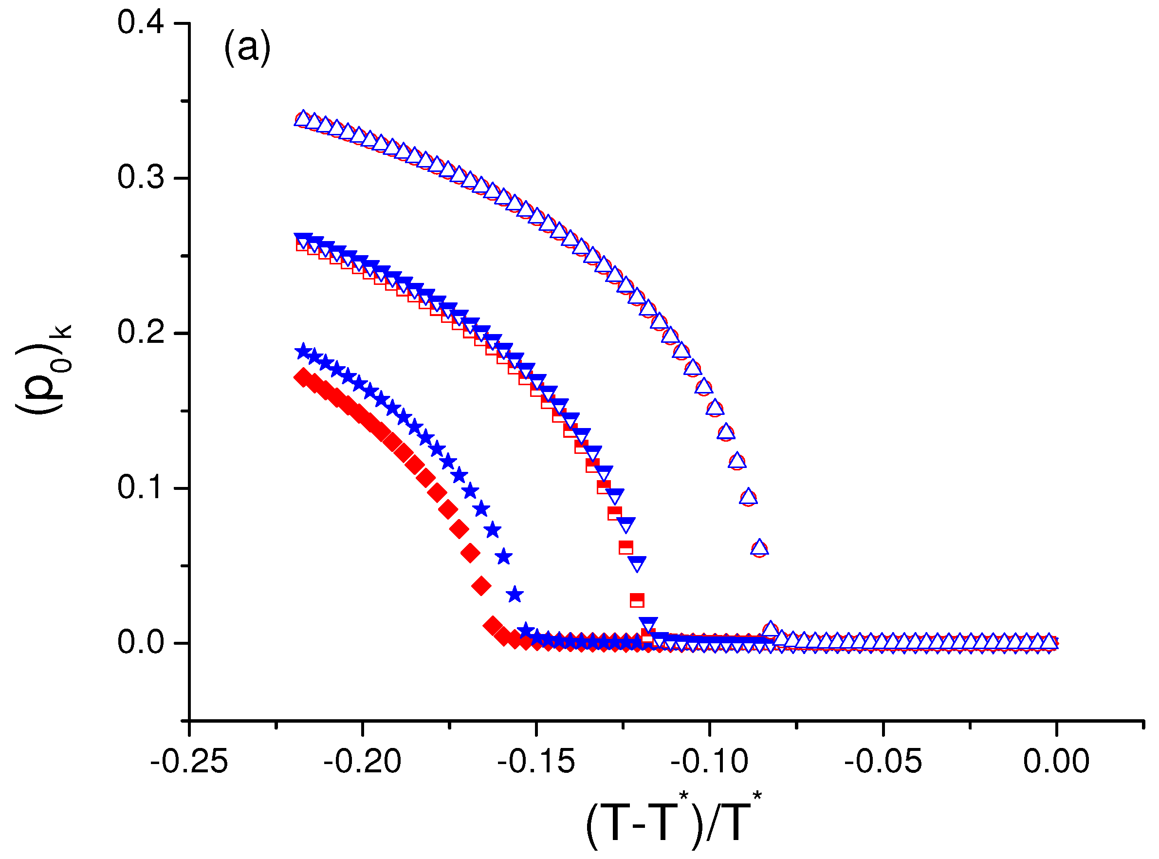
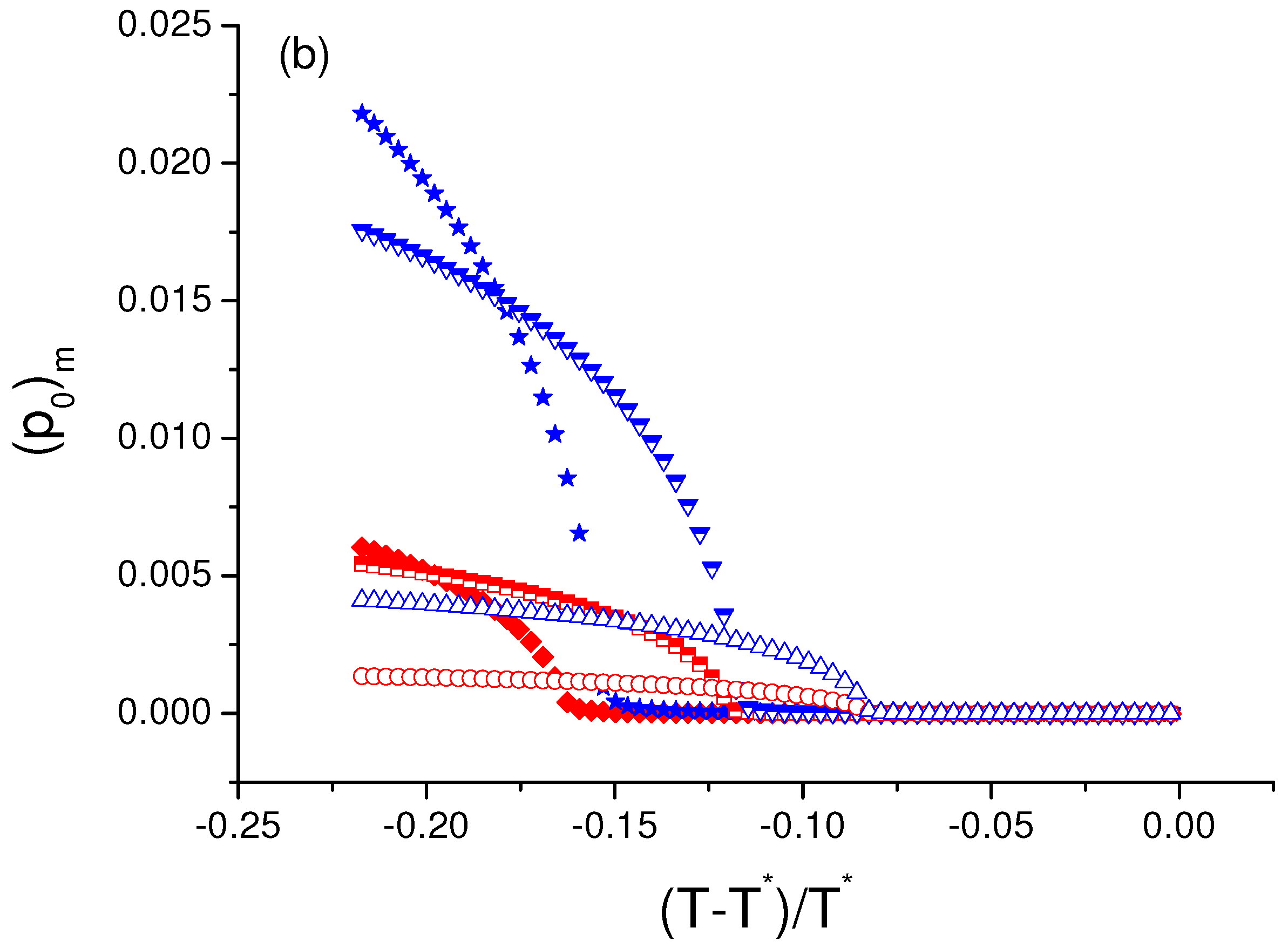
where $P_i(\mathbf{a}·\mathbf{n})$ are the Legendre polynomials. One notes that Equation (16) always has trivial solution ${\mathbf{p}}_0=\mathbf{0}$. At the same time, it is noticeable already from Equation (15) that large positive tensor element ${\widehat{\mathbf{g}}}_{kk}^{+}$ in both synclinic and anticlinic phases [see Equations (8) and (14)] can cause different from zero solution for projection ${\left({\mathbf{p}}_0\right)}_k$ at sufficiently large tilt angle, since parameter $g_1={\mu }_{\mathrm{ef}}^2/\left(2{cos}^3\theta \right)$ increases with the increasing tilt angle. Element ${\widehat{\mathbf{g}}}_{kk}^{+}$ is positive [13,14,15], because projections of polarizations on the smectic layer normal have favorable head-and-tail coupling, while the side-by-side coupling of projections of polarizations on the smectic layer plane is either completely not favorable (in the synclinic phase) or is not that favorable (in the anticlinic phase), and the corresponding elements ${\widehat{\mathbf{g}}}_{ww}^{+}$ and ${\widehat{\mathbf{g}}}_{mm}^{+}$ are either negative (in the synclinic phase) or positive, but approximately twice smaller (in the anticlinic phase). Temperature dependencies of polarizations ${\left({\mathbf{p}}_0\right)}_k$ and ${\left({\mathbf{p}}_0\right)}_m$ corresponding to solutions to Equation (16) are presented in Figure 4 for several values of the order parameters $S_2$ and $S_4$, while polarization ${\left({\mathbf{p}}_0\right)}_w$ always appears to be equal to zero. So far we assume that both synclinic and anticlinic phases can exist at each temperature, while determination of which particular phase should indeed exist at particular temperature requires the comparison of their free energies that will be done in the following sections. In the manner of paper [17], we assume that the tilt angle is the only parameter explicitly depending on the temperature, mostly due to interactions not related to polarization. On the other hand, variation of polarization is driven by variation of the tilt angle participating in Equations (17) and (18) for $\widehat{\mathbf{r}}$ and $Z_0$ with temperature, while the temperature dependence of the tilt angle itself can be modeled by the following expression [17]:

$${sin}^2\theta =-\frac{\tilde{T}}{B_0-B_1\tilde{T}},$$

(20)

where $B_1^{-1}$ is the square sine function of the saturated tilt angle, ratio $B_1/B_0$ regulates how fast is the saturation with variation of temperature, and $\tilde{T}\equiv (T-T^{*})/T^{*}$ is the reduced temperature showing the deviation from temperature $T^{*}$ of transition into Sm-$A^{*}$. If both nematic order parameters $S_2$ and $S_4$ are equal to zero, the spontaneous polarization arises only along $\mathbf{k}$-axis. At the same time, if order parameters $S_2$ and/or $S_4$ are different from zero, polarization $\left({\mathbf{p}}_0\right)$ appears to be biased to the plane, which is perpendicular to director $\mathbf{n}$, and in this case polarization cannot arise solely along $\mathbf{k}$-axis, because it should have a projection on axes $\mathbf{w}$ and/or ${\mathbf{m}}^{\prime }$ (see Figure 2). Among these two projections, only the projection on ${\mathbf{m}}^{\prime }$-axis has a contribution along $\mathbf{k}$-axis, but, on the other hand, it has also a contribution along $\mathbf{m}$-axis, and therefore, both polarizations ${\left({\mathbf{p}}_0\right)}_k$ and ${\left({\mathbf{p}}_0\right)}_m$ should arise simultaneously, while polarization ${\left({\mathbf{p}}_0\right)}_w$ can be equal to zero. The transition point, at which the proper spontaneous polarization arises, corresponds to the non-trivial solution of Equation (16) at ${\mathbf{q}}_0=0$, which can be formulated in the following simple form:

$$\frac{S_2{\widehat{\mathbf{g}}}_{kk}^{+}{sin}^2\theta }{1-\frac{1}{3}(1-S_2){\widehat{\mathbf{g}}}_{kk}^{+}}+\frac{S_2{\widehat{\mathbf{g}}}_{mm}^{+}{cos}^2\theta }{1-\frac{1}{3}(1-S_2){\widehat{\mathbf{g}}}_{mm}^{+}}=2,$$

(21)

Starting from transition point the left-hand side of Equation (21) should become larger than two. Roughly speaking, to satisfy this requirement molecular system needs to have either large enough numerators [requiring large enough elements of tensor ${\widehat{\mathbf{g}}}^{+}$] or small enough denominators in the left-hand side of Equation (21). However, large tensor ${\widehat{\mathbf{g}}}^{+}$ requires large dipole moment ${\mu }_{\mathrm{ef}}$ [see Equations (8) and (14)], but our estimations show that conventional synclinic phase, which is suppressed by the same terminal dipoles [17,18], becomes unstable before the dipoles reach sufficiently large values. Therefore Equation (21) can reasonably be fulfilled only due to small denominators. The corresponding dependence of the transition tilt angle, at which the spontaneous polarization ${\mathbf{p}}_0$ arises, on the nematic order parameter of flexible tails $S_2$ is presented in Figure 5 for both synclinic and anticlinic phases. One can see that in the anticlinic phase there exist two opportunities to reach the transition point at reasonably small tilt: (1) either nematic order of flexible tails should be very small, and in this case dipoles $\mathbf{\mu }$ are not biased to the plane perpendicular to director $\mathbf{n}$ and therefore can have sufficiently large projections on the smectic layer normal $\mathbf{k}$, or (2) the nematic order of flexible tails should be very large, and in this case both projections on axes $\mathbf{k}$ and $\mathbf{m}$ [which are both favorable in the anticlinic phase] appear to be large. On the contrary, in the synclinic phase, the projections of dipoles on the $\mathbf{m}$-axis in the neighboring layers have unfavorable coupling, and only opportunity (1) exists, and therefore, the transition tilt angle monotonously increases with the increasing order parameter. We do not expect projection ${\left({\mathbf{p}}_0\right)}_m$ in the anticlinic phase to be very large, because otherwise it should cause reverse (decrease with lowering the temperature) of the tilt angle due to anti-polar side-by-side ordering of these projections in the neighboring layers and due to the head-and-tail ordering of these projections along the $\mathbf{m}$-axis within the same smectic layers. This reverse of tilt is not specific to the re-entrant ferroelectric phase, but is rather specific to hexatic and re-entrant Sm-$A^{*}$ phases, which are going to be considered in the following publications. Therefore, we do not expect the nematic ordering of flexible tails to be very large in both synclinic and anticlinic phases considered here. In the present paper, we assume that the molecular tails are essentially disordered and suppose that it is important for the formation of the re-entrant ferroelectric phase.

5. Polarization in the Presence of Electric Field: Re-Entrant Ferroelectric Phase

In the general case, when local field $\mathbf{M}$ is different from zero, polarization is expected to vary from layer to layer in the anticlinic phase. For both synclinic and anticlinic phases let us change over from polarization ${\mathbf{p}}_1$ in layer 1 and polarization ${\mathbf{p}}_2$ in layer 2 to new variables:

$$\begin{array}{c}\hfill {\mathbf{q}}_1\equiv {\widehat{\mathbf{g}}}_0{\mathbf{p}}_1+2{\widehat{\mathbf{g}}}_1{\mathbf{p}}_2,{\mathbf{q}}_2\equiv {\widehat{\mathbf{g}}}_0{\mathbf{p}}_2+2{\widehat{\mathbf{g}}}_1{\mathbf{p}}_1\end{array}$$

(22)

in the synclinic phase, or

$$\begin{array}{c}\hfill {\mathbf{q}}_1\equiv {\widehat{\mathbf{g}}}_0{\mathbf{p}}_1+2{\widehat{\mathbf{g}}}_1^A{\mathbf{p}}_2,{\mathbf{q}}_2\equiv {\widehat{\mathbf{g}}}_0{\mathbf{p}}_2+2{\widehat{\mathbf{g}}}_1^A{\mathbf{p}}_1\end{array}$$

(23)

in the anticlinic phase. Elimination of the distribution function (Equation (10)) from the free energy (Equation (7)) yields:

$$\begin{array}{cc}\frac{F_i}{\rho k_{B}T}\hfill & =-ln{Z}_1-ln{Z}_2+\frac{1}{2}{\mathbf{q}}_1{\widehat{\mathbf{g}}}_0{({\widehat{\mathbf{g}}}_0^2-4{\widehat{\mathbf{g}}}_1^2)}^{-1}{\mathbf{q}}_1\hfill \\ \hfill & +\frac{1}{2}{\mathbf{q}}_2{\widehat{\mathbf{g}}}_0{({\widehat{\mathbf{g}}}_0^2-4{\widehat{\mathbf{g}}}_1^2)}^{-1}{\mathbf{q}}_2-2{\mathbf{q}}_1{\widehat{\mathbf{g}}}_1{({\widehat{\mathbf{g}}}_0^2-4{\widehat{\mathbf{g}}}_1^2)}^{-1}{\mathbf{q}}_2,\hfill \end{array}$$

(24)

for the synclinic phase, and similar expression, where tensor ${\widehat{\mathbf{g}}}_1$ is replaced with ${\widehat{\mathbf{g}}}_1^A$, for the anticlinic phase. In both cases for $i=1,2$

$$\begin{array}{c}\hfill Z_i=\int d^2{\mathbf{a}}_{1}d{\psi }_1{f}_{0}exp({\mathbf{\mu }}_i{\mathbf{q}}_i+{\mathbf{\mu }}_i^{*}{\mathbf{M}}_i),\end{array}$$

(25)

where variables ${\mathbf{q}}_1$ and ${\mathbf{q}}_2$ are defined either in Equation (22) in case of synclinic phase or in Equation (23) in case of anticlinic phase. Expanding free energy (24) in Taylor series with respect to the local fields ${\mathbf{M}}_1$ and ${\mathbf{M}}_2$ as shown in Appendix B and taking into account that local field generally contains contribution ${\mathbf{M}}_0$, which is the same in every smectic layer, and contribution $\Delta \mathbf{M}$, which alternates in sign from layer to layer (for the synclinic phase the latter one is equal to zero), one obtains for both synclinic and anticlinic phases the following expression for the part of the free energy per one smectic layer, which explicitly depends on the local field:

$$\frac{\Delta F}{\rho k_{B}T}=-\frac{1}{2}{\mathbf{M}}_0{\widehat{\mathbf{\epsilon }}}^{+}{\mathbf{M}}_0-\frac{1}{2}\Delta \mathbf{M}{\widehat{\mathbf{\epsilon }}}^{-}\Delta \mathbf{M},$$

(26)

where ${\widehat{\mathbf{\epsilon }}}^{\pm }$ are the generalized dielectric tensors:

$$\begin{array}{c}{\widehat{\mathbf{\epsilon }}}_{\alpha \beta }^{+}\equiv \frac{1}{2}\frac{d[{\left({\mathbf{p}}_1^{*}\right)}_{\alpha }+{\left({\mathbf{p}}_2^{*}\right)}_{\alpha }]}{d{\left({\mathbf{M}}_0\right)}_{\beta }}{|}_{{\mathbf{M}}_{1,2}=\mathbf{0}},\hfill \\ {\widehat{\mathbf{\epsilon }}}_{\alpha \beta }^{-}\equiv \frac{1}{2}\frac{d[{\left({\mathbf{p}}_1^{*}\right)}_{\alpha }-{\left({\mathbf{p}}_2^{*}\right)}_{\alpha }]}{d{(\Delta \mathbf{M})}_{\beta }}{|}_{{\mathbf{M}}_{1,2}=\mathbf{0}},\hfill \end{array}$$

(27)

and in Appendix B it is shown that

$${\widehat{\mathbf{\epsilon }}}^{\pm }=\frac{{\widehat{\Delta }}^{*}{\widehat{\mathbf{g}}}^{\pm }{\widehat{\Delta }}_T^{*}}{\widehat{\mathbf{I}}+{\widehat{\mathbf{g}}}^{\pm }\widehat{\Delta }}-{\widehat{\Delta }}^{**},$$

(28)

where $\widehat{\mathbf{I}}$ is the unit tensor, ${\widehat{\mathbf{g}}}^{\pm }\equiv {\widehat{\mathbf{g}}}_0\pm 2{\widehat{\mathbf{g}}}_1$ in the synclinic phase or ${\widehat{\mathbf{g}}}^{\pm }\equiv {\widehat{\mathbf{g}}}_0\pm 2{\widehat{\mathbf{g}}}_1^A$ in the anticlinic phase, and tensors describing the dispersion of various projections of dipole moments are expressed as follows [see Appendix A]:

$$\begin{array}{cc}{\widehat{\Delta }}_{\alpha \beta }\hfill & \equiv {\left({\mathbf{p}}_0\right)}_{\alpha }{\left({\mathbf{p}}_0\right)}_{\beta }-\int d^2{\mathbf{a}}_{1}d{\psi }_{1}f{\mathbf{\mu }}_{\alpha }{\mathbf{\mu }}_{\beta }\hfill \\ \hfill & \approx {\left({\mathbf{p}}_0\right)}_{\alpha }{\left({\mathbf{p}}_0\right)}_{\beta }-\frac{1}{Z_0}\{\frac{1}{2}\left[\left(\frac{2}{3}+\frac{1}{3}{S}_2\right){\widehat{\mathbf{\delta }}}_{\alpha \beta }-S_2{\mathbf{n}}_{\alpha }{\mathbf{n}}_{\beta }\right]\hfill \\ \hfill & +\frac{1}{16}[\left(\frac{8}{15}+\frac{8}{21}{S}_2+\frac{3}{35}{S}_4\right)\left({\mathbf{q}}_0^2{\widehat{\mathbf{\delta }}}_{\alpha \beta }+2{\left({\mathbf{q}}_0\right)}_{\alpha }{\left({\mathbf{q}}_0\right)}_{\beta }\right)\hfill \\ \hfill & -\left(\frac{4}{7}{S}_2+\frac{3}{7}{S}_4\right)(2\left(\mathbf{n}{\mathbf{q}}_0\right)({\left({\mathbf{q}}_0\right)}_{\alpha }{\mathbf{n}}_{\beta }+{\mathbf{n}}_{\alpha }{\left({\mathbf{q}}_0\right)}_{\beta })\hfill \\ \hfill & +{\left(\mathbf{n}{\mathbf{q}}_0\right)}^2{\widehat{\mathbf{\delta }}}_{\alpha \beta }+{\mathbf{q}}_0^2{\mathbf{n}}_{\alpha }{\mathbf{n}}_{\beta })+3S_4{\left(\mathbf{n}{\mathbf{q}}_0\right)}^2{\mathbf{n}}_{\alpha }{\mathbf{n}}_{\beta }]\},\hfill \end{array}$$

(29)

$$\begin{array}{cc}{\widehat{\Delta }}_{\alpha \beta }^{*}\hfill & ={\left({\widehat{\Delta }}_T^{*}\right)}_{\beta \alpha }\equiv {\left({\mathbf{p}}_0^{*}\right)}_{\alpha }{\left({\mathbf{p}}_0\right)}_{\beta }-\int d^2{\mathbf{a}}_{1}d{\psi }_{1}f{\mathbf{\mu }}_{\alpha }^{*}{\mathbf{\mu }}_{\beta }\hfill \\ \hfill & \approx -\frac{1}{2Z_0}\{\frac{1}{2}(1+S_1){\widehat{\mathbf{\delta }}}_{\alpha \beta }+\left[\frac{1}{96}(5+S_2)+\frac{1}{64}(S_1+3S_3)\right]\hfill \\ \hfill & \times [2{\left({\mathbf{q}}_0\right)}_{\alpha }{\left({\mathbf{q}}_0\right)}_{\beta }+{\mathbf{q}}_0^2{\widehat{\mathbf{\delta }}}_{\alpha \beta }]-\left[\frac{1}{48}(2+S_2)-\frac{1}{32}(S_1-3S_3)\right]\hfill \\ \hfill & \times [2\left(\mathbf{n}{\mathbf{q}}_0\right){\left({\mathbf{q}}_0\right)}_{\alpha }{\mathbf{n}}_{\beta }+{\left(\mathbf{n}{\mathbf{q}}_0\right)}^2{\widehat{\mathbf{\delta }}}_{\alpha \beta }]\},\hfill \end{array}$$

(30)

$$\begin{array}{cc}{\widehat{\Delta }}_{\alpha \beta }^{**}\hfill & \equiv {\left({\mathbf{p}}_0^{*}\right)}_{\alpha }{\left({\mathbf{p}}_0^{*}\right)}_{\beta }-\int d^2{\mathbf{a}}_{1}d{\psi }_{1}f{\mathbf{\mu }}_{\alpha }^{*}{\mathbf{\mu }}_{\beta }^{*}\hfill \\ \hfill & \approx -\frac{1}{2Z_0}\{{\widehat{\mathbf{\delta }}}_{\alpha \beta }+\frac{1}{48}(2+S_2)[2{\left({\mathbf{q}}_0\right)}_{\alpha }{\left({\mathbf{q}}_0\right)}_{\beta }+3{\mathbf{q}}_0^2{\widehat{\mathbf{\delta }}}_{\alpha \beta }]\hfill \\ \hfill & +\frac{1}{16}{S}_1[2{\left({\mathbf{q}}_0\right)}_{\alpha }{\left({\mathbf{q}}_0\right)}_{\beta }-{\mathbf{q}}_0^2{\widehat{\mathbf{\delta }}}_{\alpha \beta }]\hfill \\ \hfill & +\frac{1}{48}(2-11S_2){\left(\mathbf{n}{\mathbf{q}}_0\right)}^2{\widehat{\mathbf{\delta }}}_{\alpha \beta }\},\hfill \end{array}$$

(31)

where $f\equiv f_i({\mathbf{M}}_i=\mathbf{0})=f_{0}exp\left(\mathbf{\mu }{\mathbf{q}}_0\right)/Z_0$, ($i=1,2$) [see Equations (10), (22) and (23)], and where we neglected in advance all terms, which are orthogonal to vectors ${\mathbf{M}}_0$ and $\Delta \mathbf{M}$ and participate in scalar products with these vectors in Equation (26). Counting azimuthal orientation $\phi$ of the normal to the local tilt plane from the direction of external electric field, one obtains instead of Equation (9) the following expression for the local filed:

$$\begin{array}{c}{\mathbf{M}}_w=c_{p}cos\theta sin\theta +2c_{f}h{\phi }^{\prime }sin\theta \pm {\mu }^{*}Ecos\phi /\left(k_{B}T\right),\hfill \\ {\mathbf{M}}_m=\mp {\mu }^{*}E{cos}^2\theta sin\phi /\left(k_{B}T\right)\hfill \\ {\mathbf{M}}_k=\pm {\mu }^{*}Esin\theta cos\theta sin\phi /\left(k_{B}T\right),\hfill \end{array}$$

(32)

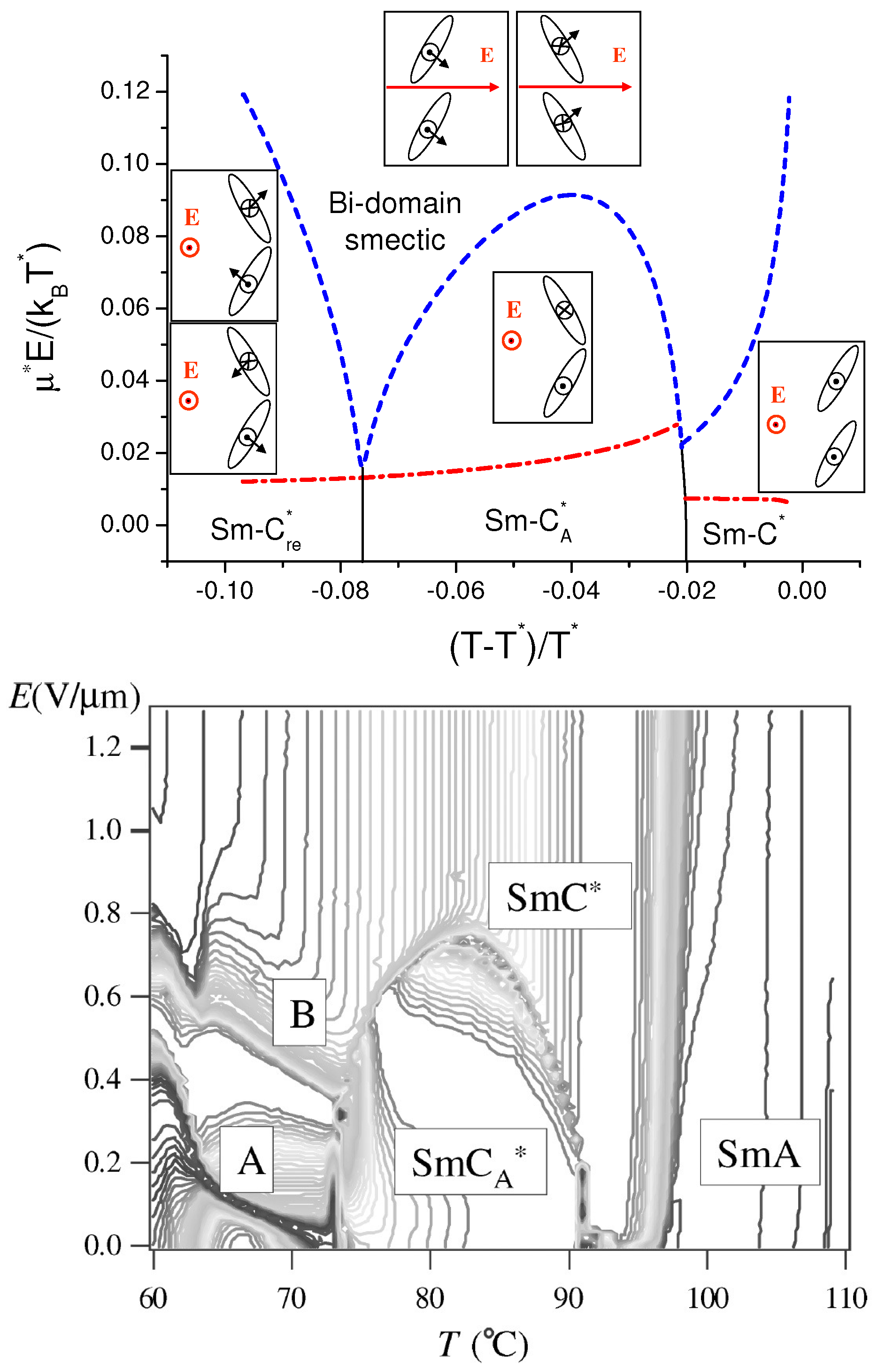
where h is the layer spacing and ${\phi }^{\prime }$ is the derivative of the azimuthal orientation with respect to coordinate z along the smectic layer normal $\mathbf{k}$. In the case of synclinic phase the upper sign in Equation (32) should be taken for each layer, while in the case of anticlinic phase the upper sign should be taken for layer 1, and the lower sign should be taken for layer 2. Thus, in the anticlinic phase, a part of the local field explicitly depending on external electric field E alternates in sign from layer to layer and therefore contributes into the second term of Equation (26) for the free energy. On the contrary, in the synclinic phase electric field E contributes into the first term of Equation (26). One notes from Equation (28) for the generalized dielectric tensor that element ${\left({\widehat{\mathbf{\epsilon }}}^{+}\right)}_{kk}$ diverges exactly at the same transition point, where the proper spontaneous polarization ${\left({\mathbf{p}}_0\right)}_k$ arises in the synclinic phase, i.e., where constraint (21) is fulfilled. From comparison of the free energies it follows that the transition point belongs to the temperature interval, where the anticlinic phase has lower free energy without electric field. Below and above this point ${\left({\widehat{\mathbf{\epsilon }}}^{+}\right)}_{kk}$ reaches very large positive values, which means that in the vicinity of the transition into the proper ferroelectric phase the favorable coupling of induced polarizations along smectic layer normal $\mathbf{k}$ in the neighboring smectic layers is very strong in the synclinic phase. On the contrary, element ${\left({\widehat{\mathbf{\epsilon }}}^{-}\right)}_{kk}$ does not diverge at the same point and is negative in the vicinity of this point, which means that induced polarization in the anticlinic phase would exhibit unfavorable coupling along the smectic layer normal $\mathbf{k}$ in the neighboring smectic layers if projection of induced polarization along axis $\mathbf{k}$ existed. This difference expressed by elements ${\left({\widehat{\mathbf{\epsilon }}}^{+}\right)}_{kk}$ and ${\left({\widehat{\mathbf{\epsilon }}}^{-}\right)}_{kk}$ reflects the two tendencies: (1) in the vicinity of transition into the proper ferroelectric phase, the coupling between induced polarizations along the smectic layer normal $\mathbf{k}$ favors orientation of the tilt planes along the electric field direction in the synclinic phase, and perpendicular to the electric field direction in the anticlinic phase, because ${\mathbf{M}}_k^2$ is proportional to ${sin}^2\phi$ [see Equation (32)]; (2) the same coupling promotes transition from the anticlinic phase to the synclinic one in the presence of electric field. In particular, at the temperature corresponding to transition into the proper ferroelectric phase exactly, very small electric field causes the synclinic structure. We suppose that without the electric field, the proper ferroelectric phase with spontaneous polarization along the smectic layer normal is anticlinic and can correspond to the observed experimentally re-entrant ferroelectric phase Sm-$C_{\mathrm{re}}^{*}$, while above this point in the temperature scale, the conventional antiferroelectric phase Sm-$C_A^{*}$ is observed. The entire Electric field–Temperature phase diagram is presented in Figure 6a, where solid black thin lines detach Sm-$C_{\mathrm{re}}^{*}$, Sm-$C_A^{*}$ and Sm-$C^{*}$, dash blue thick line detaches the mentioned above phases from the bidomain synclinic smectic phase with the tilt plane projections either along or against the electric field, and dash dot red thick line detaches the helical phases from the unwound ones [see details in the following sections]. Black arrows inside molecules show the direction of polarization ${\mathbf{p}}^{*}$.

Insets for Sm-$C_{\mathrm{re}}^{*}$ and for the synclinic phase arising above the dash blue thick line show that both mentioned phases can possess the two kinds of domains with two opposite orientations of polarization projection on the smectic layer normal. As mentioned in the introduction, the interaction of dipoles in the neighboring smectic layers essentially influences their orientation, especially when polarization increases in the electric field. Since the dipole–dipole interaction is proportional to the dipole squared, while the interaction of all dipoles with electric field is proportional to the first power of molecular dipole moment, the dipole–dipole interaction can sufficiently influence the value and orientation of polarization at large electric field. In the tilted smectic phase, a part of the transverse molecular dipoles have always non-zero projections on the smectic layer normal, whose “head-and-tail” configuration is the most favorable and is very important in correspondence with Equation (3). One notes, however, that the transverse molecular dipoles have both non-zero contributions along the smectic layer normal and along the electric field direction only if the tilt planes are not perpendicular to the electric field. When the dipole moments become sufficiently large (due to the presence of electric field), the free energy appears to be lower if the molecular system realizes the “head-and-tail” projections for the larger number of molecular dipoles, and the tilt planes start reorienting partially in the direction along the electric field (or against the electric field). Because of this, the polarization has non-zero projections as along the electric field, as along the smectic layer normal. The larger the electric field, the larger the deviation of the tilt planes from perpendicular to the electric field orientation. These questions were considered accurately in Refs. [13,14,15]. Most likely, the opposite domains in both Sm-$C^{*}$ and Sm-$C_{\mathrm{re}}^{*}$ are the solitons whose dimension is determined by prehistory of their creation. The corresponding experimental phase diagram is presented in Figure 6b, which is reproduced with permission from Ref. [8]. One notes a very good coincidence of the phase transition borders in both Figure 6a,b.

6. Temperature Induced Transition Between Synclinic And Anticlinic Smectic Phases

It is believed that synclinic-anticlinic phases transition in tilted smectics is driven mostly by polarization-independent part of the free energy [18]. Here we are going to follow this idea and will use the same semi-phenomenological expression for the polarization-independent free energy, as in [12,13,14,15,17]:

$$\begin{array}{cc}\frac{F_0}{\rho k_{B}T}\hfill & =\left(\frac{3}{2}{v}_1-\frac{1}{4}{g}_1^2+4c_f^2\right)\sum _{i=0}^{t-1}{({\mathbf{n}}_i·{\mathbf{n}}_{i+1})}^2\hfill \\ \hfill & +\left(v_3+\frac{3}{2}{g}_1^2\right){cos}^2\theta \sum _{i=0}^{t-1}({\mathbf{n}}_i·{\mathbf{n}}_{i+1})\hfill \\ \hfill & +v_5\sum _{i=0}^{t-1}({\mathbf{n}}_i·{\mathbf{n}}_{i+1})(\mathbf{k}·[{\mathbf{n}}_i\times {\mathbf{n}}_{i+1}]),\hfill \end{array}$$

(33)

where the terms proportional to coefficients $v_1$ and $v_3$ describe the non-chiral dispersion interactions, the term proportional to $v_5$ describes the chiral dispersion interaction, the terms proportional to $g_1^2$ represent the dipole–dipole interaction treated in the second virial expansion, and the term proportional to $c_f^2$ represents the dipole-quadrupole interaction treated in the second virial expansion. Equation (33) can be rewritten in terms of tilt angle $\theta$ and azimuthal rotation $\Delta \phi$ of the director from layer to layer:

$$\begin{array}{cc}\frac{F_0}{\rho k_{B}T}\hfill & =b{sin}^4\theta {cos}^2\Delta \phi +\frac{1}{4}a{sin}^2\left(2\theta \right)cos\Delta \phi \hfill \\ \hfill & +c{sin}^2\theta sin\Delta \phi (1+cos\Delta \phi ),\hfill \end{array}$$

(34)

where

$$\begin{array}{c}a\equiv (3v_1+v_3)+g_1^2+8c_f^2,\\ b\equiv \frac{3}{2}{v}_1-\frac{1}{4}{g}_1^2+4c_f^2,c\equiv v_5.\end{array}$$

(35)

Most often the dispersion contributions $v_1$ and $3v_1+v_3$ are negative, which promotes the formation of the synclinic phase Sm-$C^{*}$ [minimum of Equation (34) is close to $\Delta \phi =0$ if helicity c is small]. At the same time, parameters $g_1^2$ and $c_f^2$ are positive, which promotes anticlinic smectic phase Sm-$C_A^{*}$ [minimum of Equation (34) is close to $\Delta \phi =\pi$]. Thus, a competition between the dispersion and the electrostatic forces can generate a transition from synclinic phase to anticlinic phase, when the temperature decreases, because parameter $g_1^2={\mu }_{\mathrm{ef}}^4/\left(4{cos}^6\theta \right)$ increases with the increasing tilt angle (decreasing temperature), and has no tendency of reversal. In other words, there is no objective reason for reappearance of synclinic phase at low temperatures, and therefore, the re-entrant ferroelectric phase Sm-$C_{\mathrm{re}}^{*}$ most likely appears to be anticlinic, although projections of polarization on the smectic layer normal can exhibit synpolar ordering in this phase, as was discussed in the previous section.

7. Helical Rotation, Elasticity and Deformation of Sm-${\mathbf{C}}^{*}$, Sm-${\mathbf{C}}_{\mathit{A}}^{*}$ and Sm-${\mathbf{C}}_{\mathrm{Re}}^{*}$ in the Electric Field

Replacing $\Delta \phi$ with $h{\phi }^{\prime }$ in Equation (34) in the case of synclinic phase or with $\pi +h{\phi }^{\prime }$ in the case of anticlinic phase, substituting local field [Equation (32)] into Equation (26), and combining Equations (26) and (34) for polarization-dependent and polarization-independent parts of the free energy, one obtains the following well-known expression for the total free energy of the distorted smectic phase in the presence of electric field explicitly depending on the azimuthal distribution of director from layer to layer:

$$\frac{F(\phi ,{\phi }^{\prime })}{\rho k_{B}T}=f_0+\frac{1}{2}K{\left(\frac{\partial \phi }{\partial z}-q_0\right)}^2-\lambda Ecos\phi -\nu E^2{sin}^2\phi ,$$

(36)

where, however, we can estimate all the parameters for both synclinic and anticlinic phases in terms of the dielectric tensor ${\widehat{\mathbf{\epsilon }}}^{\pm }$ [Equation (28)] and parameters a, b and c [Equation (35)]:

$$\begin{array}{cc}{f}_0+\frac{1}{2}K{q}_0^2\hfill & =b{sin}^4\theta \pm a{sin}^2\theta {cos}^2\theta \hfill \\ \hfill & -\frac{1}{2}{c}_p^2{\widehat{\mathbf{\epsilon }}}_{ww}^{+}{sin}^2\theta {cos}^2\theta -\frac{1}{2}{\left(\frac{{\mu }^{*}E}{k_{B}T}\right)}^2{\widehat{\mathbf{\epsilon }}}_{ww}^{\pm }\hfill \end{array}$$

(37)

is the free energy of the unwound structure of particular phase (which is independent of the helical rotation and orientation of the sample),

$$\begin{array}{c}\hfill \frac{K}{h^2}=-2b{sin}^4\theta \mp a{sin}^2\theta {cos}^2\theta -4c_f^2{\widehat{\mathbf{\epsilon }}}_{ww}^{+}{sin}^2\theta \end{array}$$

(38)

is the twist elastic constant,

$$\begin{array}{c}\hfill \frac{K{q}_0}{h}=-c{sin}^2\theta (1\pm {cos}^2\theta )+2c_p{c}_f{\widehat{\mathbf{\epsilon }}}_{ww}^{+}{sin}^2\theta cos\theta \end{array}$$

(39)

is the equilibrium helical wave number at $E=0$ multiplied by K determined in Equation (38),

$$\begin{array}{cc}\nu \hfill & =\frac{1}{2}{\left(\frac{{\mu }^{*}}{k_{B}T}\right)}^2[-{\widehat{\mathbf{\epsilon }}}_{ww}^{\pm }+{\widehat{\mathbf{\epsilon }}}_{mm}^{\pm }{cos}^4\theta +{\widehat{\mathbf{\epsilon }}}_{kk}^{\pm }{sin}^2\theta {cos}^2\theta \hfill \\ \hfill & -({\widehat{\mathbf{\epsilon }}}_{mk}^{\pm }+{\widehat{\mathbf{\epsilon }}}_{km}^{\pm })sin\theta {cos}^3\theta ],\hfill \end{array}$$

(40)

is the dielectric constant resulting from anisotropy of coupling between induced polarizations in the neighboring smectic layers. In Equations (37)–(40) the upper sign corresponds to the synclinic phase, while the lower sign corresponds to the anticlinic phase. Finally, parameter $\lambda$ determining an influence of the electric field on the spontaneous polarization is equal to zero in the anticlinic phase, while in the synclinic phase it is determined by the following expression:

$$\lambda =\frac{c_p{\mu }^{*}}{k_{B}T}{\widehat{\mathbf{\epsilon }}}_{ww}^{+}sin\theta cos\theta$$

(41)

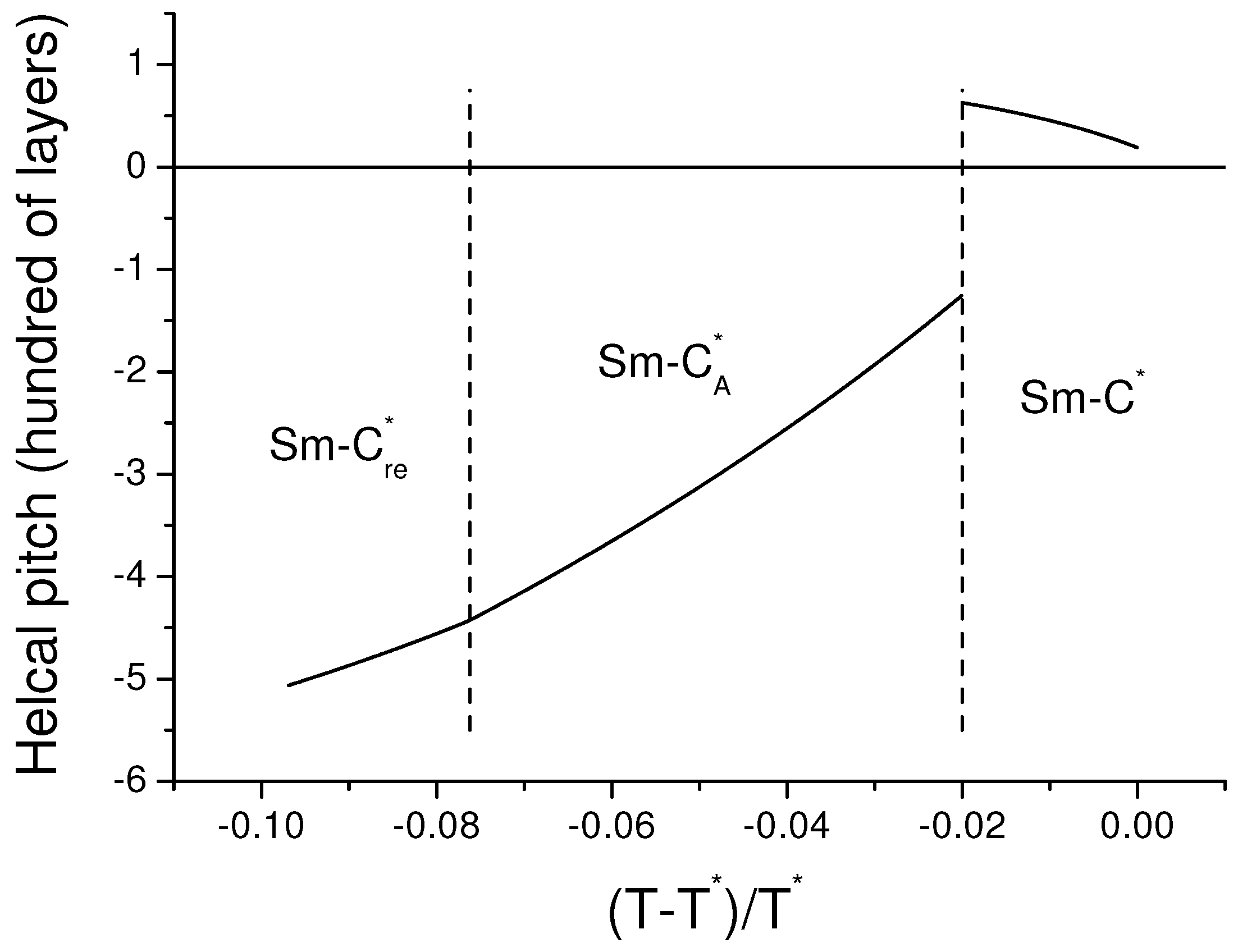
Deformation of the helical smectic structure with free energy (36) is considered explicitly in [13]. It was shown that there should be the two thresholds in each phase in the presence of electric field. The first one corresponds to the critical unwinding electric field, and the second one corresponds to the reorientation of the molecular tilt planes along the electric field direction. It was shown that, for example, in the anticlinic phase, the second threshold coincides with the electric field induced transition into synclinic phase. Here we confirm that the same is valid for Sm-$C_{\mathrm{re}}^{*}$. Both thresholds are shown in the phase diagram presented in Figure 6a. The temperature dependence of the helical pitch in each phase in the absence of electric field derived from Equations (38) and (39) is presented in Figure 7, from where it follows that there should be no discontinuous jump of the helical pitch between Sm-$C_A^{*}$ and Sm-$C_{\mathrm{re}}^{*}$. At the same time, the discontinuous jump together with helical sense inversion happens between Sm-$C_A^{*}$ and Sm-$C^{*}$.

8. Dielectric Response

To validate our supposition about the anticlinic structure of Sm-$C_{\mathrm{re}}^{*}$, let us estimate the dielectric response in Sm-$C^{*}$, Sm-$C_A^{*}$ and Sm-$C_{\mathrm{re}}^{*}$. According to Equation (27), the local polarization induction due to the presence of local field (9) in the synclinic phase is equal to

$$\Delta {\mathbf{p}}^{*}={\widehat{\mathbf{\epsilon }}}^{+}{\mathbf{M}}_0,$$

(42)

while in the anticlinic phase it is equal to:

$$\Delta {\mathbf{p}}^{*}={\widehat{\mathbf{\epsilon }}}^{-}{(\Delta \mathbf{M})}_{\Vert }+{\widehat{\mathbf{\epsilon }}}^{+}{\left({\mathbf{M}}_0\right)}_{\perp },$$

(43)

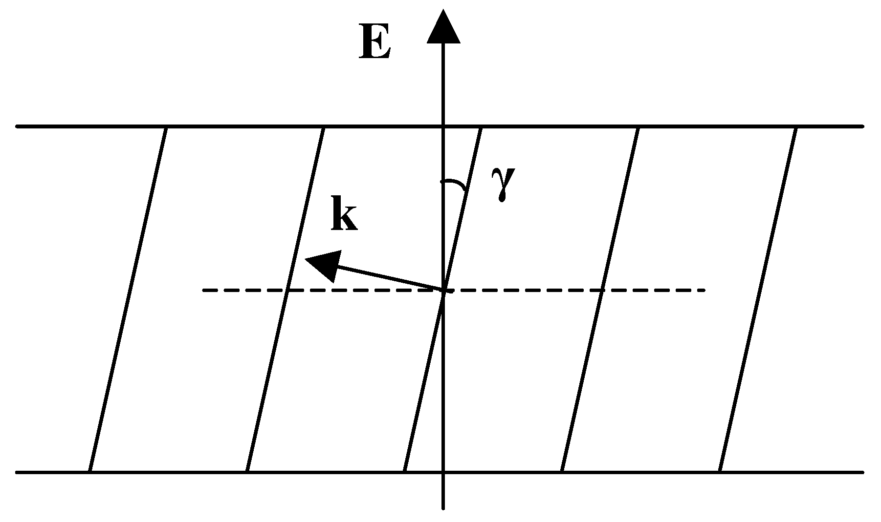
where ${(\Delta \mathbf{M})}_{\Vert }$ is the projection of $\Delta \mathbf{M}$ on the smectic layer plane and ${\left({\mathbf{M}}_0\right)}_{\perp }$ is the projection of ${\mathbf{M}}_0$ on the smectic layer normal. To estimate the dielectric effect, which is measured experimentally, one needs to estimate the polarization induction in the direction of electric field. Equation (32) for the local field assumes that the smectic layers are perpendicular to the electric field. In the presence of spontaneous polarization ${\left({\mathbf{p}}_0\right)}_k$ along the smectic layer normal, however, we expect that external electric field should cause a deformation of smectic layers (Figure 8), so that the smectic layer normal should gain a contribution $sin\gamma$ along electric field $\mathbf{E}$. The corresponding contribution to the free energy consists of the interaction of polarization ${\left({\mathbf{p}}_0\right)}_k$ with electric field and elasticity energy:

$$\frac{\Delta F_{\gamma }}{\rho k_{B}T}\approx -\frac{{\mu }^{*}E}{k_{B}T}{\left({\mathbf{p}}_0^{*}\right)}_{k}sin\gamma +\frac{1}{2}{K}_{\gamma }{sin}^2\gamma ,$$

(44)

where by analogy to Equations (16) and (17) spontaneous polarization ${\mathbf{p}}_0^{*}$ is determined by the following equation:

$$\begin{array}{cc}{\mathbf{p}}_0^{*}\hfill & =\frac{1}{2Z_0}\{\frac{1}{2}(1+S_1)[{\mathbf{q}}_0-\left(\mathbf{n}{\mathbf{q}}_0\right)\mathbf{n}]\hfill \\ \hfill & +\left[\frac{1}{96}(5+S_2)+\frac{1}{64}(S_1+3S_3)\right]{\mathbf{q}}_0^3\hfill \\ \hfill & -\left[\frac{1}{48}(2+S_2)-\frac{1}{32}(S_1-3S_3)\right]{\left(\mathbf{n}{\mathbf{q}}_0\right)}^2{\mathbf{q}}_0\hfill \\ \hfill & -\left[\frac{1}{96}(5+S_2)+\frac{1}{64}(S_1+3S_3)\right]{\mathbf{q}}_0^2\left(\mathbf{n}{\mathbf{q}}_0\right)\mathbf{n}\hfill \\ \hfill & +\left[\frac{1}{48}(2+S_2)-\frac{1}{32}(S_1-3S_3)\right]{\left(\mathbf{n}{\mathbf{q}}_0\right)}^3\mathbf{n}\}.\hfill \end{array}$$

(45)

Minimization of the free energy [(Equation (44)] yields

$$sin\gamma \approx \frac{1}{K_{\gamma }}\frac{{\mu }^{*}E}{k_{B}T}{\left({\mathbf{p}}_0\right)}_k,$$

(46)

and the corresponding addition to the local field [(Equation (32)] will be

$${\left({\mathbf{M}}_{\gamma }\right)}_k=\frac{{\mu }^{*}E}{k_{B}T}sin\gamma$$

(47)

Changing over from the local coordinate system to the laboratory one, combining the basic local field [(Equation (32)] with addition [(Equation (47)], one obtains the following expression for the polarization induction along the direction of the external electric field in the synclinic phase:

$$\begin{array}{cc}\Delta {\mathbf{p}}_E^{*}\hfill & ={\widehat{\mathbf{\epsilon }}}_{ww}^{+}(c_{p}sin\theta cos\theta +2c_{f}h{\phi }^{\prime }sin\theta )cos\gamma cos\phi \hfill \\ \hfill & +\frac{{\mu }^{*}E}{k_{B}T}\{{cos}^2\gamma [{\widehat{\mathbf{\epsilon }}}_{ww}^{+}{cos}^2\phi +cos\theta {sin}^2\phi ({\widehat{\mathbf{\epsilon }}}_{mm}^{+}cos\theta \hfill \\ \hfill & -{\widehat{\mathbf{\epsilon }}}_{mk}^{+}sin\theta \left)\right]-sin\gamma cos\gamma sin\phi [{\widehat{\mathbf{\epsilon }}}_{mk}^{+}+cos\theta ({\widehat{\mathbf{\epsilon }}}_{km}^{+}cos\theta \hfill \\ \hfill & -{\widehat{\mathbf{\epsilon }}}_{kk}^{+}sin\theta \left)\right]+{\widehat{\mathbf{\epsilon }}}_{kk}^{+}{sin}^2\gamma \},\hfill \end{array}$$

(48)

and in the anticlinic phase:

$$\begin{array}{cc}\Delta {\mathbf{p}}_E^{*}\hfill & =\frac{{\mu }^{*}E}{k_{B}T}\{{cos}^2\gamma [{\widehat{\mathbf{\epsilon }}}_{ww}^{-}{cos}^2\phi +cos\theta {sin}^2\phi ({\widehat{\mathbf{\epsilon }}}_{mm}^{-}cos\theta \hfill \\ \hfill & -{\widehat{\mathbf{\epsilon }}}_{mk}^{-}sin\theta \left)\right]-sin\gamma cos\gamma sin\phi [{\widehat{\mathbf{\epsilon }}}_{mk}^{+}+cos\theta ({\widehat{\mathbf{\epsilon }}}_{km}^{-}cos\theta \hfill \\ \hfill & -{\widehat{\mathbf{\epsilon }}}_{kk}^{-}sin\theta \left)\right]+{\widehat{\mathbf{\epsilon }}}_{kk}^{+}{sin}^2\gamma \},\hfill \end{array}$$

(49)

From derivation presented in [13] it follows that in the deformed helical structure

$${\left({\phi }^{\prime }\right)}^{-1}\approx \frac{1}{q_0}\left(1+\frac{\lambda E}{K{q}_0^2}cos\phi \right).$$

(50)

Integrating polarization induction Equations (48) or (49) over coordinate z along the smectic layer normal, and replacing $dz$ with ${\left({\phi }^{\prime }\right)}^{-1}d\phi$, one obtains for the static dielectric permittivity in the direction of electric field per one smectic layer in the synclinic phase:

$$\begin{array}{cc}{\epsilon }_E\hfill & =\frac{1}{2}{cos}^2\gamma [{\widehat{\mathbf{\epsilon }}}_{ww}^{+}+cos\theta ({\widehat{\mathbf{\epsilon }}}_{mm}^{+}cos\theta -{\widehat{\mathbf{\epsilon }}}_{mk}^{+}sin\theta )]\hfill \\ \hfill & +{\widehat{\mathbf{\epsilon }}}_{kk}^{+}{sin}^2\gamma +\frac{1}{2}\frac{{\left(c_p{\widehat{\mathbf{\epsilon }}}_{ww}^{+}\right)}^2}{K{q}_0^2}{sin}^2\theta {cos}^2\theta cos\gamma ,\hfill \end{array}$$

(51)

and in the anticlinic phase:

$$\begin{array}{c}\hfill {\epsilon }_E=\frac{1}{2}{cos}^2\gamma [{\widehat{\mathbf{\epsilon }}}_{ww}^{-}+cos\theta ({\widehat{\mathbf{\epsilon }}}_{mm}^{-}cos\theta -{\widehat{\mathbf{\epsilon }}}_{mk}^{-}sin\theta )]+{\widehat{\mathbf{\epsilon }}}_{kk}^{+}{sin}^2\gamma .\end{array}$$

(52)

Usually in the experiment the alternating voltage is applied and only the “slow” component of the dielectric permittivity is taken into account. In Equations (51) and (52) only terms depending on $c_p$ and/or $\gamma$ are related to the director orientation in the electric field, which is assumed to be “slow”. The other terms are related to the induced polarization, which requires only reorientation of the molecular short axes without reorientation of director. It is expected to be much faster and is usually deducted from experimental data. Thus, we can estimate approximately the experimentally observed dielectric permittivity if we consider in Equations (51) and (52) only terms depending explicitly on $c_p$ and/or $\gamma$. According to the phase diagram presented in Figure 6a, Sm-$C_{\mathrm{re}}^{*}$ is expected to possess the anticlinic stricture, and thus, the “slow” component of the dielectric permittivity in Sm-$C_{\mathrm{re}}^{*}$ is determined by the following expression:

$$\Delta {\epsilon }_E=\frac{1}{2}{sin}^2\gamma [2{\widehat{\mathbf{\epsilon }}}_{kk}^{+}-{\widehat{\mathbf{\epsilon }}}_{ww}^{-}-cos\theta ({\widehat{\mathbf{\epsilon }}}_{mm}^{-}cos\theta +{\widehat{\mathbf{\epsilon }}}_{mk}^{-}sin\theta )],$$

(53)

where deformation of layers $\gamma$ due to spontaneous polarization along the smectic layer normal arising in Sm-$C_{\mathrm{re}}^{*}$ is determined by Equation (46). In the conventional anticlinic phase Sm-$C_A^{*}$ distortion of layers $\gamma$ is equal to zero, and therefore $\Delta {\epsilon }_E$ is approximately equal to zero. In the temperature range of the conventional synclinic phase Sm-$C^{*}$ angle $\gamma$ is also equal to zero, whereas $\Delta {\epsilon }_E$ is determined by the piezoelectric spontaneous polarization:

$$\Delta {\epsilon }_E=\frac{1}{2}\frac{{\left(c_p{\widehat{\mathbf{\epsilon }}}_{ww}^{+}\right)}^2}{K{q}_0^2}{sin}^2\theta {cos}^2\theta ,$$

(54)

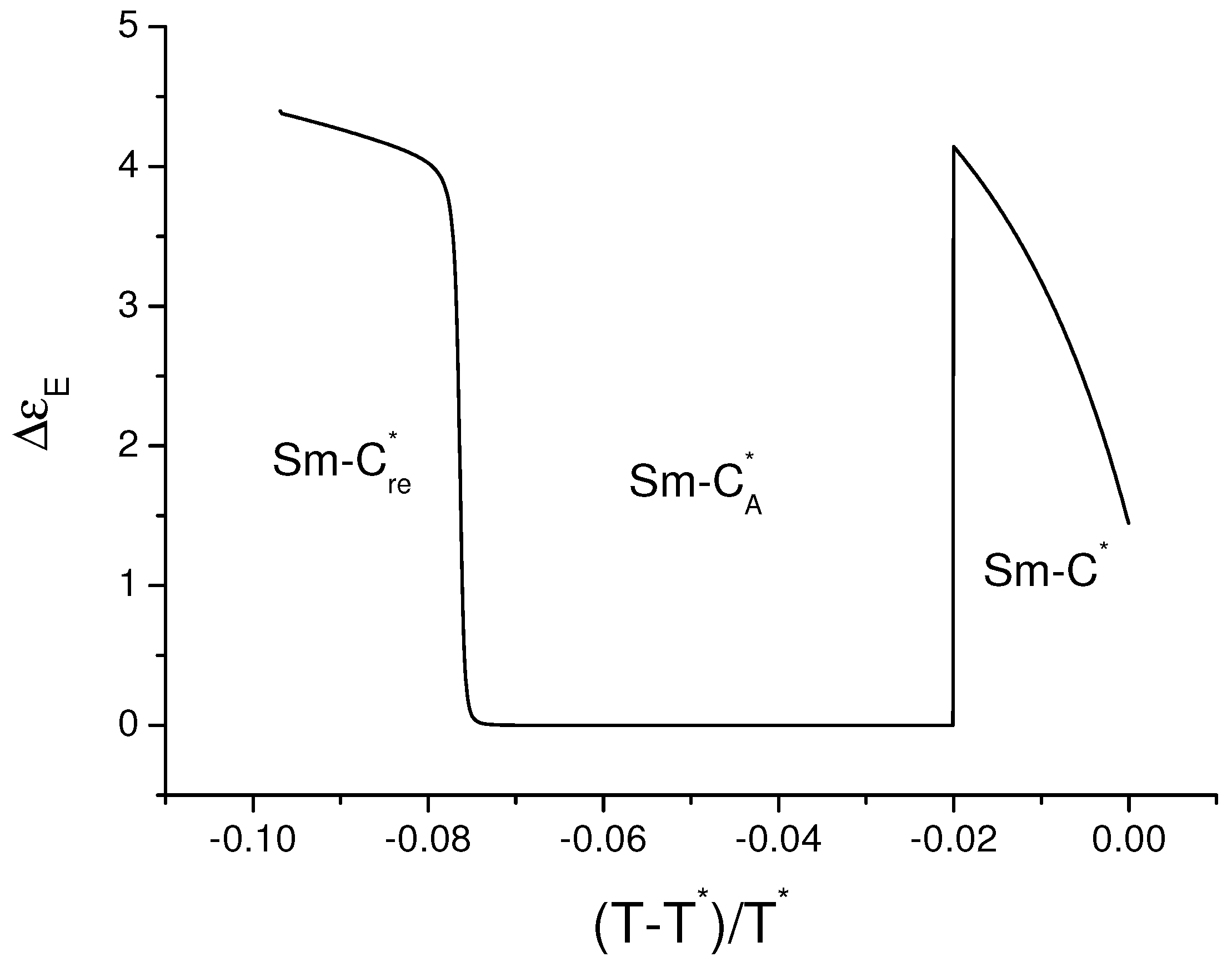
The temperature dependence of $\Delta {\epsilon }_E$ in Sm-$C^{*}$, Sm-$C_A^{*}$ and Sm-$C_{\mathrm{re}}^{*}$ is presented in Figure 9. Qualitatively it coincides with the experimentally observed dependence.

9. Conclusions

A molecular–statistical approach to the description of the re-entrant ferroelectric phase is derived. We have confirmed the experimental data [5,7,8,9,10] showing that sufficiently long molecular tails with several transverse electric dipoles near their own chiral centers promote the re-entrant ferroelectric phase observed in lactic acid derivatives [3,4]. If the prime orientational order of the flexible tails is small, the dipoles in the molecular tails can make considerable contribution to the polarization arising spontaneously along the smectic layer normal. This effect is suggested to be the origin for the re-entrant ferroelectric phase. It is shown that Sm-$C_{\mathrm{re}}^{*}$ can arise solely due to the dipole–dipole interaction, and thus, in contrast to the conventional (improper) ferroelectric Sm-$C^{*}$, appears to be the proper ferroelectric phase.

A model of a jump rope was considered for the interpretation of rigidness of the flexible tails with respect to rotation around their prime local orientation. As a result of this rigidness, the transverse electric dipoles located in the molecular tails can rotate only together with transverse electric dipoles located in the molecular core. Since the molecular tails are long and flexible in prime direction, the transverse dipoles located in the molecular tails can generally point in any direction, including the direction along the smectic layer normal. In this case, the "head-and-tail" configuration of the dipoles located nearby each other in the neighboring smectic layers can be realized, and this configuration appears to be the most favorable from the point of view of their interaction. Below particular temperature, this interaction induces the non-zero average orientation of dipoles, and thus, the proper spontaneous polarization arises. However, the polarization of molecular tails themselves, pointing perpendicular to the smectic layer surfaces, is expected to be small. At the same time, because of the rigidness of the molecular tails with respect to their rotation around their prime axes, the azimuthal orientation of this polarization is automatically transmitted into the molecular core, and a large proper spontaneous polarization arises because of the presence of transverse electric dipoles in the molecular core. Since the molecular tilt (which can be specified for the rigid molecular core) is usually not very large, the spontaneous polarization related to the molecular cores (but formed because of the transmission from the molecular tails) has generally large projection on smectic layer surface, and, as a result, can be manipulated by the electric field applied along the surfaces of smectic layers.

Since the layer spacing decreases with the reducing temperature, it is reasonable to propose that the distance between all dipoles also reduces. The distance between each pair of interacting dipoles participates in the denominator of the dipole–dipole interaction, and therefore the existence or the absence of proper ferroelectricity in particular material can also depend on the temperature. Experimental observations show that the re-entrant ferroelectric phase (which is obviously different by nature from the conventional improper ferroelectric phase) is observed only in particular materials and only in the temperature range, which is below the range of conventional ferroelectric and antiferroelectric phases. The typical parameters of theory, which are used in previous publication by the author, confirm this scenario. We have also considered the nematic ordering of the molecular tails and have demonstrated that the best coincidence with experiment (the largest temperature of transition into the proper ferroelectric phase) should be observed at the complete nematic disorder of the molecular tails, which is only possible if they are sufficiently long. Thus, without electric field, the sequence of phases with the decreasing temperature in smectic material with sufficiently long flexible tails should be Sm-$A^{*}$, Sm-$C^{*}$, Sm-$C_A^{*}$, and Sm-$C_{\mathrm{re}}^{*}$. Here we use the stars in abbreviation of all phases to reflect their chirality, although the chirality itself is not mandatory for the existence of any of these phases, but is important for the existence of the improper spontaneous polarization. In the case of chiral molecules, the helical rotation of director should be observed in any of these phases, and in the present paper, in particular, we generalize the method of calculation of the helical pitch for the case of the re-entrant ferroelectric phase and demonstrate the corresponding temperature dependence of the helical pitch in various phases.

In contrast to the transition from Sm-$C^{*}$ to Sm-$C_A^{*}$, the transition between Sm-$C_A^{*}$ and Sm-$C_{\mathrm{re}}^{*}$ is the second-order phase transition. The normal to the smectic layers polarization gives large negative contribution to the free energies of both synclinic and anticlinic phases, but in the synclinic phase the longitudinal to the smectic layers polarization is not favorable, and therefore, the re-entrant ferroelectric phase appears to be anticlinic. However, due to the presence of polarization in the direction of the smectic layer normal in Sm-$C_{\mathrm{re}}^{*}$ (this polarization is synpolar in each smectic layer), the smectic layer surfaces should exhibit a deformation in the electric field resulting in the dielectric response. In the present paper, we have calculated the corresponding dielectric permittivity, which appeared to be of the same order of magnitude, as in the conventional ferroelectric phase. This fact is also confirmed experimentally.

Finally, the general electric field–temperature phase diagram is calculated reflecting the behavior of each phase in the electric filed. As one can see from Figure 6, theoretical phase diagram almost coincides with the experimental one [8]. Moreover, from our theory we can reconstruct the of the Sm-$C^{*}$, Sm-$C_A^{*}$, and Sm-$C_{\mathrm{re}}^{*}$ phases in the electric field, while experimentally sometimes we can only fix the transitions without detailed information about the structure. In all the tilted phases the unwinding of the helical pitch in the electric field happens first. When the electric field farther increases, the transition into the bidomain synclinic phase happens. This transition is related to the fact that molecular tilt planes start reorienting either along or against the electric field. In this case, both the projections of the transverse dipoles– along the electric field and along the smectic layer normal–can coexist. The latter ones are important for the transverse dipoles located in the molecular tails, because the most favorable “head-and-tail” configuration can be realized for the dipoles located nearby each other in the neighboring smectic layers. In the presence of electric field, the transverse molecular dipoles are redistributed to enlarge the spontaneous polarization. In particular, more dipoles tend to be in the “head-and tail” configuration in the neighboring smectic layer. As a result, at some value of electric field (depending on the temperature) the tilt planes start partial reorientation either along or against the electric field, and the two equiprobable domains arise. The re-entrant ferroelectric phase also appears to consist of the two equiprobable domains, because the two directions of the surface layer normal along which the proper polarization arises are also equivalent. In the electric field the bidomain proper anticlinic ferroelectric phase exhibits a transition into the bidomain synclinic ferroelectric phase, and this transition is clearly seen at the experimental phase diagram [Figure 6b] as the border between anomalies A and B. In particular, we have found out that at the Sm-$C_A^{*}$–Sm-$C_{\mathrm{re}}^{*}$ transition temperature exactly, the infinitely small electric field is needed to induce the transition from the bidomain anticlinic ferroelectric phase into the bidomain synclinic ferroelectric phase, which means that at this particular temperature the free energies of these two phases coincide, and both phases can coexist.

References

- Meyer, R.B. Ferroelectric Liquid Crystals. Mol. Cryst. Liq. Cryst. 1977, 36, 69–71. [Google Scholar] [CrossRef]
- Chandani, A.D.L.; Gorecka, E.; Ouchi, Y.; Takezoe, H.; Fukuda, A. Antiferroelectric Chiral Smectic Phases Responsible for the Tristable Switching in MHPOBC. Jpn. J. Appl. Phys. 1989, 28, L1265. [Google Scholar] [CrossRef]
- Novotna, V.; Hamplova, V.; Kaspar, M.; Glogarova, M.; Bubnov, A.; Lhotakova, Y. Phase diagrams of binary mixtures of antiferroelectric and ferroelectric compounds with lactate units in the mesogenic core. Ferroelectrics 2004, 309, 103–109. [Google Scholar] [CrossRef]
- Bubnov, A.; Novotna, V.; Hamplova, V.; Kaspar, M.; Glogarova, M. Effect of multilactate chiral part of the liquid crystalline molecule on mesomorphic behaviour. J. Mol. Struct. 2008, 892, 151–157. [Google Scholar] [CrossRef]
- Novotna, V.; Glogarova, M.; Hamplova, V.; Kaspar, M. Re-entrant ferroelectric phases in binary mixtures of ferroelectric and antiferroelectric homologues of a series with three chiral centers. J. Chem. Phys. 2001, 115, 9036–9041. [Google Scholar] [CrossRef]
- Bubnov, A.; Kaspar, M.; Hamplova, V.; Glogarova, M.; Samaritani, S.; Galli, G.; Andersson, G.; Komitov, L. New polar liquid crystalline monomers with two and three lactate groups for preparation of side chain polysiloxanes. Liq. Cryst. 2006, 33, 559–566. [Google Scholar] [CrossRef]
- Kaspar, M.; Hamplova, V.; Novotna, V.; Glogarova, M.; Pociecha, D.; Vanek, P. New series of ferroelectric liquid crystals with two or three chiral centres exhibiting antiferroelectric and hexatic phases. Liq. Cryst. 2001, 28, 1203–1207. [Google Scholar]
- Na, Y.; Naruse, Y.; Fukuda, N.; Orihara, H.; Fajar, A.; Hamplova, V.; Kaspar, M.; Glogarova, M. E-T Phase Diagrams of an Antiferroelectric Liquid Crystal with Re-Entrant Smectic C* Phase. Ferroelectrics 2008, 364, 13–19. [Google Scholar] [CrossRef]
- Catalano, D.; Domenici, V.; Marini, A.; Veracini, C.A.; Bubnov, A.; Glogarova, M. Structural and orientational properties of the ferro, antiferroelectric, and re-entrant smectic C* phases of ZLL7* by Deuterium NMR and other experimental techniques. J. Phys. Chem. B 2006, 110, 16459–16470. [Google Scholar] [CrossRef] [PubMed]
- Domenici, V.; Marini, A.; Menicagli, R.; Veracini, C.A.; Bubnov, A.M.; Glogarova, M. Dynamic behaviour of a ferroelectric liquid crystal by means of Nuclear Magnetic Resonance and Dielectric Spectroscopy. In Proceedings of the SPIE 6587, Liquid Crystals and Applications in Optics, Prague, Czech Republic, 16–19 April 2007; Volume 6587, p. 65871F1. [Google Scholar]
- Domenici, V.; Bubnov, A.; Marini, A.; Hamplova, V.; Kaspar, M.; Glogarova, M.; Veracini, C.A. The ferroelectric SmC* phase studied by means of 2H and 13C NMR: structural and orientational features. In Proceedings of the 37th Topical Meeting of the German Liquid Crystal Society, Stuttgart, Germany, 1–3 April 2009; pp. 115–116. [Google Scholar]
- Emelyanenko, A.V. Molecular-ststistical approach to a behaviour of ferroelectric, antiferroelectric and ferrielectric smectic phases in the electric field. Eur. Phys. J. E 2009, 28, 441–455. [Google Scholar] [CrossRef] [PubMed]
- Emelyanenko, A.V. Theory for the evolution of ferroelectric, antiferroelectric, and ferrielectric smectic phases in the electric field. Phys. Rev. E 2010, 82, 031710. [Google Scholar] [CrossRef] [PubMed]
- Emelyanenko, A.V.; Ishikawa, K. Smooth transitions between biaxial intermediate smectic phases. Soft Matter 2013, 9, 3497–3508. [Google Scholar] [CrossRef]
- Emelyanenko, A.V. Induction of new ferrielectric smectic phases in the electric field. Ferroelectrics 2016, 495, 129–142. [Google Scholar] [CrossRef]
- Emelyanenko, A.V.; Osipov, M.A. Theoretical model for the discrete flexoelectric effect and a description for the sequence of intermediate smectic phases with increasing periodicity. Phys. Rev. E 2003, 68, 0517033. [Google Scholar] [CrossRef]
- Emelyanenko, A.V.; Fukuda, A.; Vij, J.K. Theory of the intermediate tilted smectic phases and their helical rotation. Phys. Rev. E 2006, 74, 011705. [Google Scholar] [CrossRef] [Green Version]
- Emelyanenko, A.V.; Filimonova, E.S. Molecular-statistical approach to the description of tilted smectic phases. Phase Transit. 2018, 91, 984–993. [Google Scholar] [CrossRef]
Figure 1.
Molecular formulae for ZLL materials.
Figure 2.
(Color online) Molecular model: is the laboratory frame; is the local frame related to molecular core, where axis is perpendicular to the tilt plane of director ; is the local frame related to molecular tail, where axis is perpendicular to the tilt plane of tail axis . Inset (a) shows the projection on the director tilt plane, and inset (b) shows the projection on the tilt plane of tail axis.
Figure 3.
(Color online) Positional correlation of terminal molecular dipoles. Dipoles located in the cores are essentially larger, but they do not correlate.
Figure 4.
(Color online) Spontaneous polarization along axis (a) and along axis (b) as a function of reduced temperature at and (red circles for the synclinic phase and blue up triangles for the anticlinic phase); (red rectangles and blue down triangles, respectively); (red diamonds and blue stars, respectively). Here is the transition temperature into Sm-; ; .
Figure 5.
Transition tilt angle, at which the proper spontaneous polarization arises, as a function of nematic order parameter of flexible tails at in the synclinic phase (1) and in the anticlinic phase (2).
Figure 6.
(Color online) (a) Electric field–Temperature phase diagram at , , , , , , , , , ; . Here is the phase transition temperature into Sm-, solid black thin lines detach Sm-, Sm- and Sm-, dash blue thick line detaches the above phases from the bidomain synclinic smectic phase with tilt plane projections either along or against the electric field, and dash dot red thick line detaches helical phases from the unwound ones. Black arrows inside molecules show the direction of polarization ; (b) Experimental phase diagram–reproduced with permission from Ref. [8]. Copyright Taylor and Francis, 2008.
Figure 7.
Equilibrium helical pitch at in Sm-, Sm- and Sm- at , , , , , , , , , ; . Here is the phase transition temperature into Sm-.
Figure 8.
Deformation of smectic layers in electric field in the presence of spontaneous polarization along smectic layer normal .
Figure 9.
Dielectric permittivity related to reorientation of spontaneous polarization in the electric field in Sm-, Sm- and Sm- at , , , , , , , , , ; , . Here is the phase transition temperature into Sm-.
© 2019 by the author. Licensee MDPI, Basel, Switzerland. This article is an open access article distributed under the terms and conditions of the Creative Commons Attribution (CC BY) license (http://creativecommons.org/licenses/by/4.0/).
Share and Cite
MDPI and ACS Style
Emelyanenko, A.V. Molecular–Statistical Theory for the Description of Re-Entrant Ferroelectric Phase. Crystals 2019, 9, 583. https://0-doi-org.brum.beds.ac.uk/10.3390/cryst9110583
AMA Style
Emelyanenko AV. Molecular–Statistical Theory for the Description of Re-Entrant Ferroelectric Phase. Crystals. 2019; 9(11):583. https://0-doi-org.brum.beds.ac.uk/10.3390/cryst9110583
Chicago/Turabian StyleEmelyanenko, Alexander V. 2019. "Molecular–Statistical Theory for the Description of Re-Entrant Ferroelectric Phase" Crystals 9, no. 11: 583. https://0-doi-org.brum.beds.ac.uk/10.3390/cryst9110583
Note that from the first issue of 2016, this journal uses article numbers instead of page numbers. See further details here.