
Comparative Analysis of Machine Learning and Numerical Modeling for Combined Heat Transfer in Polymethylmethacrylate

 , , and
Abstract
:1. Introduction
2. Materials and Methods
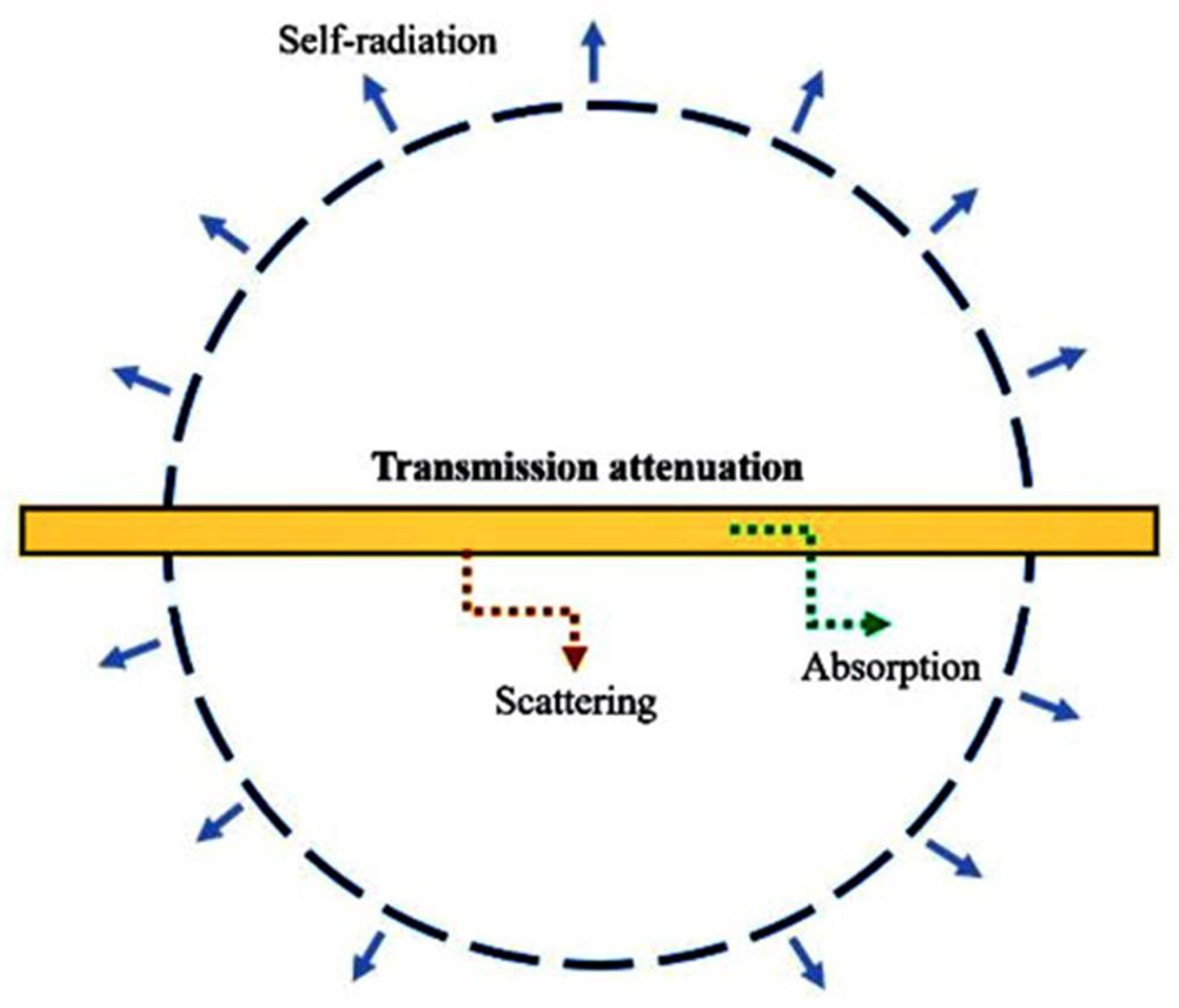
2.1. Numerical Analysis
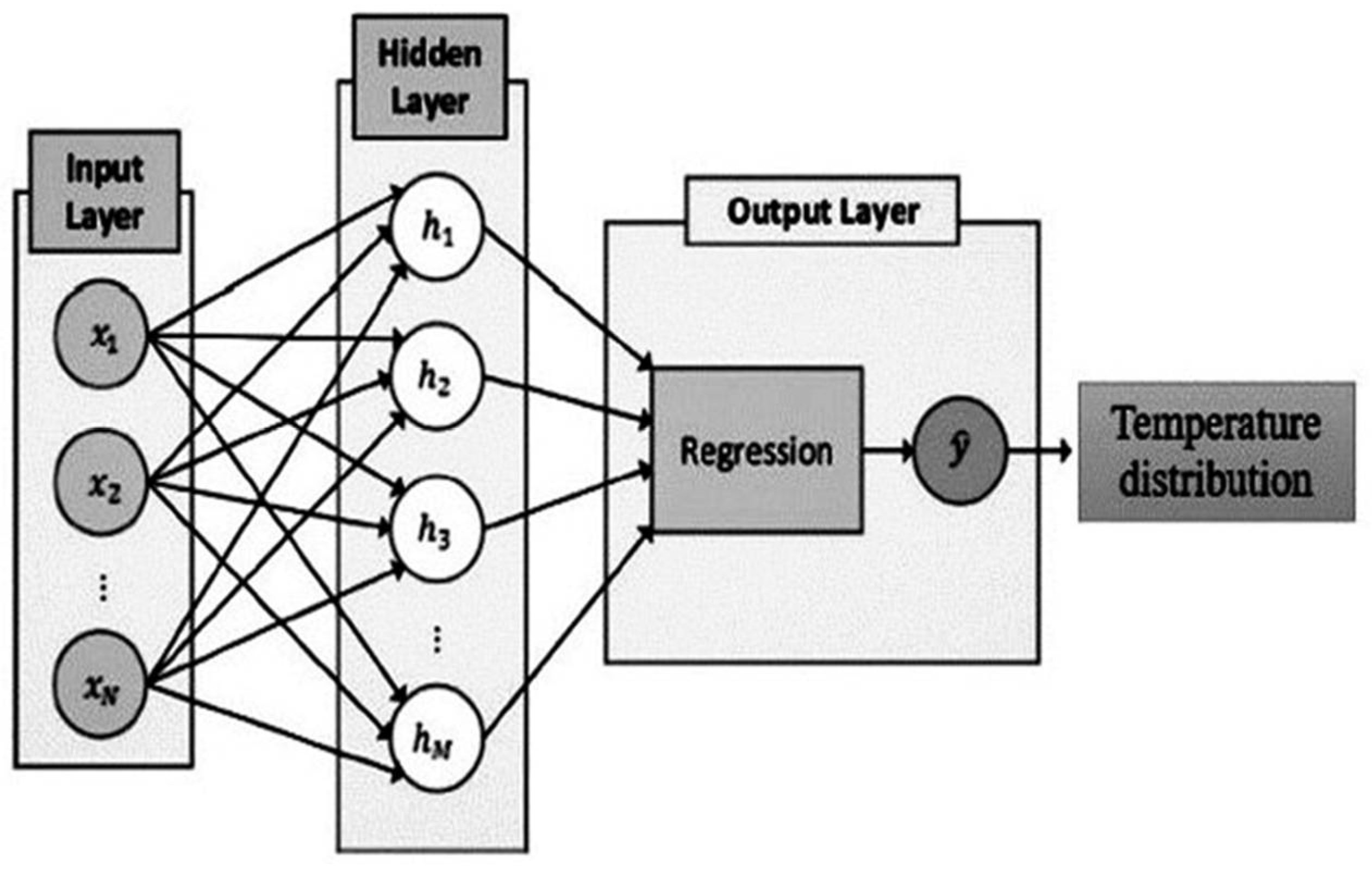
2.2. Deep Neural Network Method
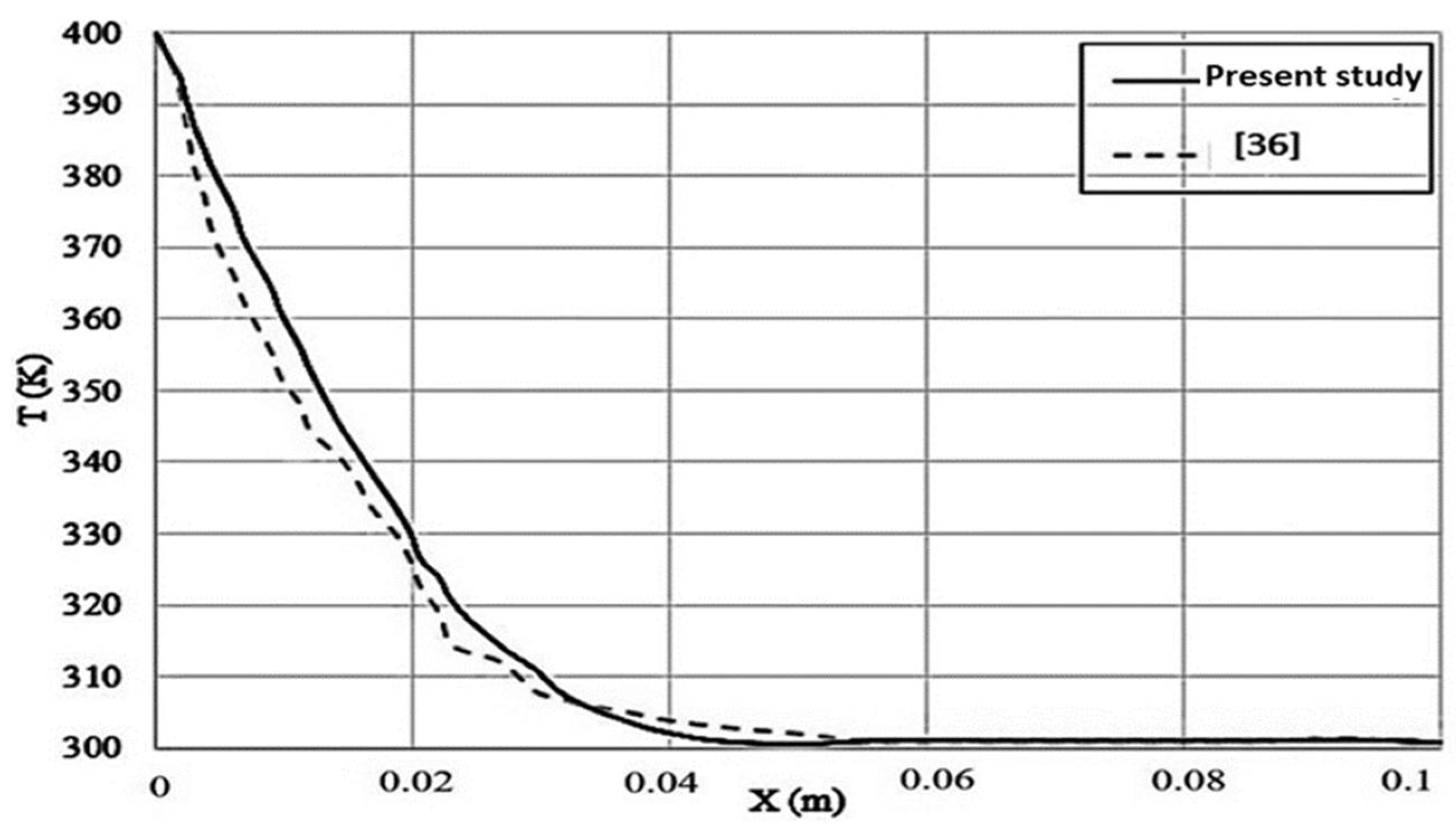
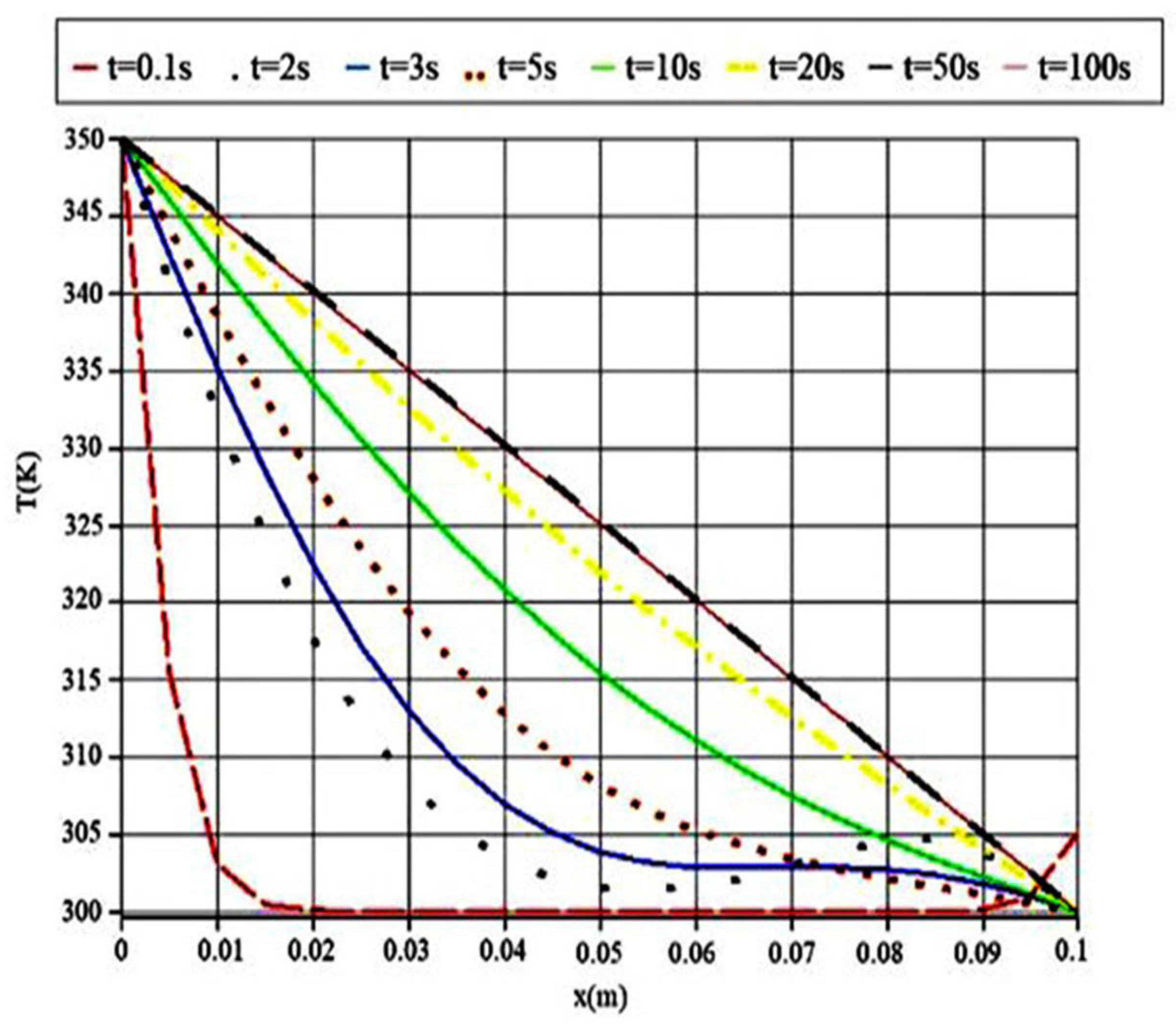
3. Results and Discussion
4. Conclusions
Author Contributions
Funding
Institutional Review Board Statement
Informed Consent Statement
Data Availability Statement
Conflicts of Interest
Nomenclature
| Parameter | Description | Parameter | Description |
| Monochromic radiation intensity | Radiative heat flux | ||
| wave length | Heat source flux | ||
| t | time | I | Radiation intensity |
| X | direction | E | Fibrous media length |
| direction | f | forget gate | |
| c | propagation speed | i | input gate |
| density | g | Non-linear sigmoid function | |
| Specific heat | O | cell-state output parameter | |
| T | Temperature | W | Weight function |
| K | thermal conductivity | Recent gate information |
References
- Yang, D.; Yu, J.; Tao, X.; Tam, H.Y. Structural and mechanical properties of polymeric optical fiber. Mater. Sci. Eng. A 2004, 364, 256–259. [Google Scholar] [CrossRef]
- Suchorab, Z.; Franus, M.; Barnat-Hunek, D. Properties of Fibrous Concrete Made with Plastic Optical Fibers from E-Waste. Materials 2020, 13, 2414. [Google Scholar] [CrossRef] [PubMed]
- Yuan, H.; Wang, Y.; Zhao, R.; Liu, X.; Bai, Q.; Zhang, H.; Gao, Y.; Jin, B. An anti-noise composite optical fiber vibration sensing System. Opt. Lasers Eng. 2021, 139, 106483. [Google Scholar] [CrossRef]
- Chaitanya, S.; Mukherjee, G.; Banerjee, M.; Jain, A. Optical studies of Rhodamine B doped polymethyl methacrylate (PMMA) films. Mater. Today Proc. 2021, 47, 592–596. [Google Scholar] [CrossRef]
- Bzówka, J.; Grygierek, M.; Rokitowski, P. Experimental investigation using distributed optical fiber sensor measurements in unbound granular layers. Eng. Struct. 2021, 231, 111767. [Google Scholar] [CrossRef]
- Jderu, A.; Soto, M.A.; Enachescu, M.; Ziegler, D. Liquid Flow Meter by Fiber-Optic Sensing of Heat Propagation. Sensors 2021, 21, 355. [Google Scholar] [CrossRef]
- Al Abdulaal, T.; Yahia, I. Optical linearity and nonlinearity, structural morphology of TiO2-doped PMMA/FTO polymeric nanocomposite films: Laser power attenuation. Optik 2021, 227, 166036. [Google Scholar] [CrossRef]
- Jatoi, A.S.; Khan, F.S.; Mazari, S.A.; Mubarak, N.M.; Abro, R.; Ahmed, J.; Ahmed, M.; Baloch, H.; Sabzoi, N. Current applications of smart nanotextiles and future trends. In Nanosensors and Nanodevices for Smart Multifunctional Textiles; Elsevier: Amsterdam, The Netherlands, 2021; pp. 343–365. [Google Scholar]
- Mousavi, S.M.; Ghasemi, M.; Dehghan Manshadi, M.; Mosavi, A. Deep learning for wave energy converter modeling using long short-term memory. Mathematics 2021, 9, 871. [Google Scholar] [CrossRef]
- Hemath, M.; Rangappa, S.M.; Kushvaha, V.; Dhakal, H.N.; Siengchin, S. A comprehensive review on mechanical, electromagnetic radiation shielding, and thermal conductivity of fibers/inorganic fillers reinforced hybrid polymer composites. Polym. Compos. 2020, 41, 3940–3965. [Google Scholar] [CrossRef]
- Sallam, O.; Madbouly, A.; Elalaily, N.; Ezz-Eldin, F. Physical properties and radiation shielding parameters of bismuth borate glasses doped transition metals. J. Alloy. Compd. 2020, 843, 156056. [Google Scholar] [CrossRef]
- Li, D.; Zhang, C.; Li, Q.; Liu, C.; Arıcı, M.; Wu, Y. Thermal performance evaluation of glass window combining silica aerogels and phase change materials for cold climate of China. Appl. Therm. Eng. 2020, 165, 114547. [Google Scholar] [CrossRef]
- Barnoss, S.; Aribou, N.; Nioua, Y.; El Hasnaoui, M.; Achour, M.E.; Costa, L.C. Dielectric Properties of PMMA/PPy Composite Materials. In Nanoscience and Nanotechnology in Security and Protection against CBRN Threats; Springer: Dordrecht, The Netherlands, 2020; pp. 259–271. [Google Scholar]
- Sans, M.; Schick, V.; Parent, G.; Farges, O. Experimental characterization of the coupled conductive and radiative heat transfer in ceramic foams with a flash method at high temperature. Int. J. Heat Mass Transf. 2020, 148, 119077. [Google Scholar] [CrossRef] [Green Version]
- Malek, M.; Izem, N.; Mohamed, M.S.; Seaid, M.; Wakrim, M. Numerical solution of Rosseland model for transient thermal radiation in non-grey optically thick media using enriched basis functions. Math. Comput. Simul. 2021, 180, 258–275. [Google Scholar] [CrossRef]
- Satapathy, A.K.; Nashine, P. Solving Transient Conduction and Radiation Using Finite Volume Method. Int. J. Mech. Mechatron. Eng. 2015, 8, 645–649. [Google Scholar]
- Wakif, A. A Novel Numerical Procedure for Simulating Steady MHD Convective Flows of Radiative Casson Fluids over a Horizontal Stretching Sheet with Irregular Geometry under the Combined Influence of Temperature-Dependent Viscosity and Thermal Conductivity. Math. Probl. Eng. 2020, 2020. [Google Scholar] [CrossRef]
- Makinde, O.D. Free convection flow with thermal radiation and mass transfer past a moving vertical porous plate. Int. Commun. Heat Mass Transf. 2005, 32, 1411–1419. [Google Scholar] [CrossRef]
- Chu, Y.-M.; Nazeer, M.; Khan, M.I.; Hussain, F.; Rafi, H.; Qayyum, S.; Abdelmalek, Z. Combined impacts of heat source/sink, radiative heat flux, temperature dependent, thermal conductivity on forced convective Rabinowitsch fluid. Int. Commun. Heat Mass Transf. 2021, 120, 105011. [Google Scholar] [CrossRef]
- Hernandez, D.; Denis, Y. Energy Management System Industrialization for Off-Grids Power Systems Based on Data-Driven Machine Learning Models. Sustain. Energy Grids Netw. 2021, preprint. [Google Scholar] [CrossRef]
- Kwon, B.; Ejaz, F.; Hwang, L.K. Machine learning for heat transfer correlations. Int. Commun. Heat Mass Trans. 2020, 116, 104694. [Google Scholar] [CrossRef]
- Manshadi, M.D.; Ghasemi, M.; Mousavi, S.M.; Mosavi, A. Predicting the Related Parameters of Vortex Bladeless Wind Turbine by Using Deep Learning Method. Available online: https://www.preprints.org/manuscript/202106.0242/v1 (accessed on 13 March 2022).
- Zhao, J.; Ye, F. Where ThermoMesh meets ThermoNet: A machine learning based sensor for heat source localization and peak temperature estimation. Sens. Actuators A Phys. 2019, 292, 30–38. [Google Scholar] [CrossRef]
- Mousavi, M.; Manshadi, M.D.; Soltani, M.; Kashkooli, F.M.; Rahmim, A.; Mosavi, A.; Kvasnica, M.; Atkinson, P.M.; Kovács, L.; Koltay, A.; et al. Modeling the efficacy of different anti-angiogenic drugs on treatment of solid tumors using 3D computational modeling and machine learning. Comput. Biol. Med. 2022, 146, 105511. [Google Scholar] [CrossRef] [PubMed]
- Ju, S.; Shimizu, S.; Shiomi, J. Designing thermal functional materials by coupling thermal transport calculations and machine learning. J. Appl. Phys. 2020, 128, 161102. [Google Scholar] [CrossRef]
- Acakpovi, A.; Matoumona, P.L.M.V. Comparative analysis of plastic optical fiber and glass optical fiber for home networks. In Proceedings of the 2012 IEEE 4th International Conference on Adaptive Science & Technology (ICAST), Kumasi, Ghana, 25–27 October 2012. [Google Scholar]
- Siegel, R. Thermal Radiation Heat Transfer; CRC Press: Boca Raton, FL, USA, 2001. [Google Scholar]
- Lockhat, R. Physics: Wheatstone bridge. S. Afr. J. Anaesth. Analg. 2020, 26, S100–S101. [Google Scholar] [CrossRef]
- Modest, M.F. Radiative Heat Transfer; Academic Press: Cambridge, MA, USA, 2013. [Google Scholar]
- Ozisik, M.N. Radiative transfer and interactions with conduction and convection. In Radiative Transfer and Interactions with Conduction and Convection; Wiley-Interscience: New York, NY, USA, 1973; Volume 587, p. 1973. [Google Scholar]
- Kant, K.; Shukla, A.; Sharma, A.; Biwole, P. Heat transfer studies of photovoltaic panel coupled with phase change material. Sol. Energy 2016, 140, 151–161. [Google Scholar] [CrossRef]
- Assael, M.J.; Botsios, S.; Gialou, K.; Metaxa, I.N. Thermal Conductivity of Polymethyl Methacrylate (PMMA) and Borosilicate Crown Glass BK7. Int. J. Thermophys. 2005, 26, 1595–1605. [Google Scholar] [CrossRef]
- Dehghan Manshadi, M.; Ghassemi, M.; Mousavi, S.M.; Mosavi, A.H.; Kovacs, L. Predicting the Parameters of Vortex Bladeless Wind Turbine Using Deep Learning Method of Long Short-Term Memory. Energies 2021, 14, 4867. [Google Scholar] [CrossRef]
- Duan, Z.; Yang, Y.; Zhang, K.; Ni, Y.; Bajgain, S. Improved Deep Hybrid Networks for Urban Traffic Flow Prediction Using Trajectory Data. IEEE Access 2018, 6, 31820–31827. [Google Scholar] [CrossRef]
- Zucatti, V.; Lui, H.F.S.; Pitz, D.B.; Wolf, W.R. Assessment of reduced-order modeling strategies for convective heat transfer. Numer. Heat Transfer Part A Appl. 2020, 77, 702–729. [Google Scholar] [CrossRef]
- Asllanaj, F.; Jeandel, G.; Roche, J.R.; Lacroix, D. Transient combined radiation and conduction heat transfer in fibrous media with temperature and flux boundary conditions. Int. J. Therm. Sci. 2004, 43, 939–950. [Google Scholar] [CrossRef]


| Property | Value |
|---|---|
| Density (g/cm3) | 1.18 |
| Surface Hardness | RM92 |
| Tensile Strength (MPa) | 70 |
| Flexural Modulus (GPa) | 2.9 |
| Linear Expansion (/°C × 10−5) | 7 |
| Max. Operating Temp. (°C) | 50 |
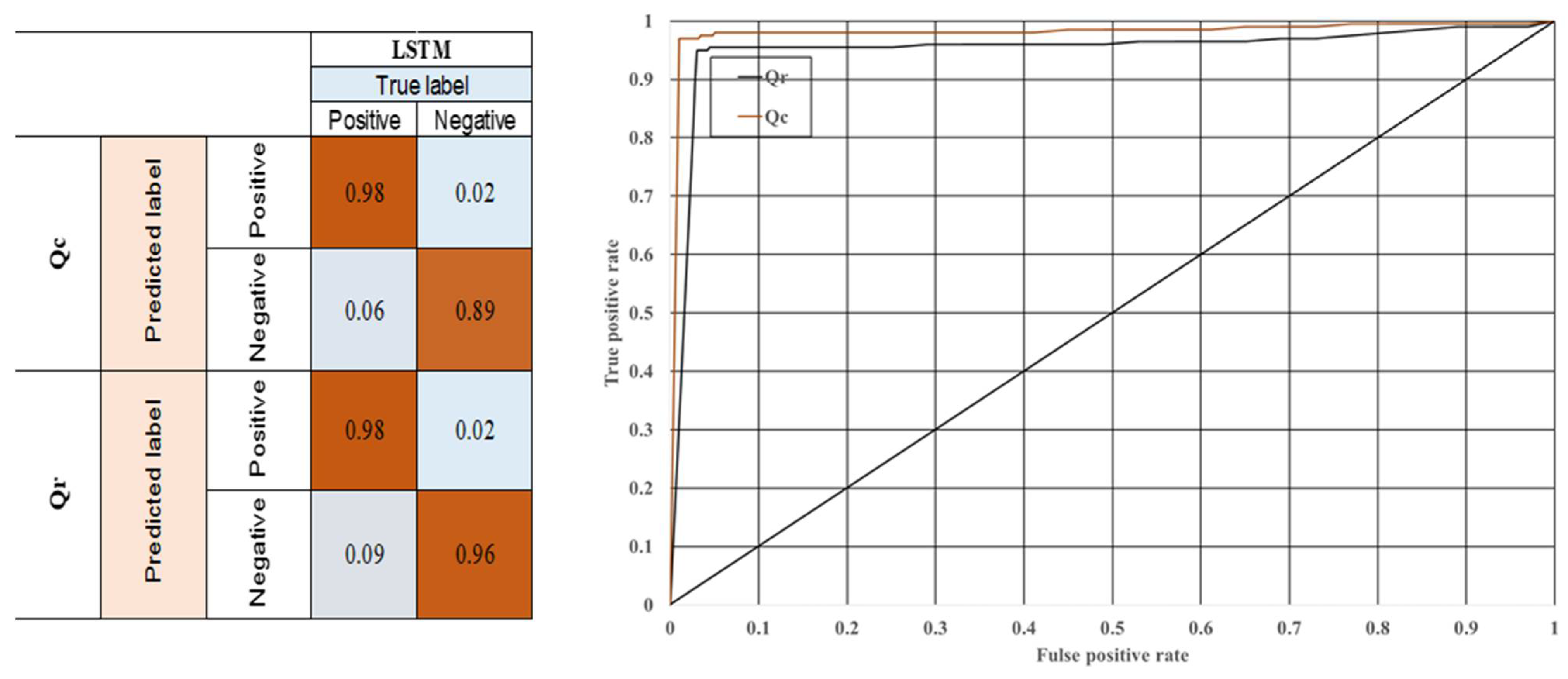
| Parameter | Method | TNR | PPV | TPR | FPR | ACC | RMSE | MAE |
|---|---|---|---|---|---|---|---|---|
| Qc | LSTM | 0.98 | 0.98 | 0.94 | 0.02 | 0.96 | 16.42 | 0.06 |
| Qr | LSTM | 0.98 | 0.98 | 0.92 | 0.02 | 0.95 | 37.53 | 0.07 |
Publisher’s Note: MDPI stays neutral with regard to jurisdictional claims in published maps and institutional affiliations. |
© 2022 by the authors. Licensee MDPI, Basel, Switzerland. This article is an open access article distributed under the terms and conditions of the Creative Commons Attribution (CC BY) license (https://creativecommons.org/licenses/by/4.0/).
Share and Cite
Dehghan Manshadi, M.; Alafchi, N.; Tat, A.; Mousavi, M.; Mosavi, A. Comparative Analysis of Machine Learning and Numerical Modeling for Combined Heat Transfer in Polymethylmethacrylate. Polymers 2022, 14, 1996. https://0-doi-org.brum.beds.ac.uk/10.3390/polym14101996
Dehghan Manshadi M, Alafchi N, Tat A, Mousavi M, Mosavi A. Comparative Analysis of Machine Learning and Numerical Modeling for Combined Heat Transfer in Polymethylmethacrylate. Polymers. 2022; 14(10):1996. https://0-doi-org.brum.beds.ac.uk/10.3390/polym14101996
Chicago/Turabian StyleDehghan Manshadi, Mahsa, Nima Alafchi, Alireza Tat, Milad Mousavi, and Amirhosein Mosavi. 2022. "Comparative Analysis of Machine Learning and Numerical Modeling for Combined Heat Transfer in Polymethylmethacrylate" Polymers 14, no. 10: 1996. https://0-doi-org.brum.beds.ac.uk/10.3390/polym14101996