A Concept of a Compact and Inexpensive Device for Controlling Weeds with Laser Beams


1
Department of Power Plants Networks and Systems, South Ural State University, 454080 Chelyabinsk City, Russia
2
Department of Plant and Environmental Sciences, Faculty of Science, University of Copenhagen, Højbakkegaard Allé 13, DK 2630 Taastrup, Denmark
*
Author to whom correspondence should be addressed.
Agronomy 2020, 10(10), 1616; https://0-doi-org.brum.beds.ac.uk/10.3390/agronomy10101616
Submission received: 1 October 2020
/
Revised: 19 October 2020
/
Accepted: 19 October 2020
/
Published: 21 October 2020
(This article belongs to the Special Issue Towards Artificially Intelligent Robotics for Agriculture – Current Developments and New Trends)
Abstract
:A prototype of a relatively cheap laser-based weeding device was developed and tested on couch grass (Elytrigia repens (L.) Desv. ex Nevski) mixed with tomatoes. Three types of laser were used (0.3 W, 1 W, and 5 W). A neural network was trained to identify the weed plants, and a laser guidance system estimated the coordinates of the weed. An algorithm was developed to estimate the energy necessary to harm the weed plants. We also developed a decision model for the weed control device. The energy required to damage a plant depended on the diameter of the plant which was related to plant length. The 1 W laser was not sufficient to eliminate all weed plants and required too long exposure time. The 5 W laser was more efficient but also harmed the crop if the laser beam became split into two during the weeding process. There were several challenges with the device, which needs to be improved upon. In particular, the time of exposure needs to be reduced significantly. Still, the research showed that it is possible to develop a concept for laser weeding using relatively cheap equipment, which can work in complicated situations where weeds and crop are mixed.
1. Introduction
Weeds are one of the most significant yield-reducing factors for crop production worldwide [1]. Herbicides have been widely used with great success since 1950s, but today, herbicide-resistant weeds are becoming an increasing problem in agriculture [2]. The extensive use of herbicides has resulted in increasing public concerns, and this has led to further restrictions for herbicide use in Europe and elsewhere [3,4], resulting in the banding of many herbicides due to risk of unwanted side-effects [5]. The possibilities of developing new effective herbicides, which can meet the environmental and safety requirements of today, seemed to be exhausted, as no new mode of action of herbicides has been developed since the 1980s [5]. This situation, together with the increasing public interest in organic food [6], calls for integrated weed management approaches to reduce weed problems in the future. Today, soil tillage and crop rotation seem to be the main alternative to herbicides [7,8]. However, soil tillage also has disadvantaged as it increases the risk of soil erosion and leaching of plant nutrients, dries out soils with limited water content, and harms beneficial soil organisms like earthworms. Flame weeding has been used in organic agricultural production but requires a large amount of gas [9] and may not be considered environmentally sustainable in the long term due to the CO2 derived production. Therefore, there is a need for developing new techniques supplementing or replacing present weed control methods [10,11].
The fast development in laser technology seems to open up new opportunities for weed control based on electricity. Laser beams can deliver high-density energy on selected spots, which warm up the plant tissue and may result in the death of the plant [12].
Heisel et al. [13] used a laser beam to cut weed stems for weed control. Treatments were carried out on greenhouse-grown pot plants at three different growth stages and from two heights. Plant dry matter was measured two to five weeks after the treatment. The relationship between dry weight and laser energy was analyzed using a non-linear dose–response regression model. They found that regrowth of weeds appeared when dicotyledonous plant stems were cut above the meristems, indicating that it is essential to cut close to the soil surface to obtain a significant effect. Marx et al. [14] proposed a weed damage model for laser irradiation, but the recognition system did only recognize one type of weeds under ideal laboratory conditions.
Mathiassen et al. [15] investigated the effect of laser treatment directed toward the apical meristems of selected weed species at the cotyledon stage. Experiments were carried out under controlled conditions using pot-grown weeds. Two lasers and two spot sizes were tested, and different energy doses were applied by varying the exposure time. The biological efficacy was examined on three different weed species (Stellaria media (L.) Vill., Tripleurospermum inodorum Sch. Bip., and Brassica napus L.). The experiments showed that laser treatment of the apical meristems caused significant growth reduction, and in some cases, killed the weed species. The biological efficacy of the laser control method was related to wavelength, exposure time, laser spot size, and laser power. The effectiveness also varied between the weed species.
Xiong et al. [16] developed a prototype robot equipped with machine vision and a gimbal- mounted laser pointers. The robot consisted of a mobile platform modified from a small commercial quad bike, a camera to detect the crop and weeds on the cotyledons stage, and two steerable gimbals controlling the laser pointers. The robot was able to identify weeds in the indoor environments and carrying lasers to irradiate the weeds. It controlled the platform in real-time realizing continuous weeding.
As several technologies have to be combined to develop a successful laser-weeding system, it may end up being costly. This paper aims to present a concept for a compact and inexpensive device for controlling weeds with laser beams. In contrast to previous research with laser weeding, we studied the effect of different laser types on relatively tall E. repens plants.
2. Materials and Methods
2.1. Weed Detection
A Raspberry Pi 3 Model B+ computer (Raspberry Pi Foundation, Cambridge, UK) with a Quad-core Broadcom BCM2837B0, Cortex-A53 64-bit SoC @ 1.4 GHz processor and 1GiB LPDDR2 SDRAM memory was applied for weed detection which is a relatively cheap and compact device. Python 3.6, vision library OpenCV 3.4.1 (The University of Birmingham, Birmingham, UK) was used as the programming language. However, the use of deep neural networks is almost impossible for quick recognition of plants due to the limited amount of RAM (14 GB) and the low processor speed (1.5 GHz) of the Raspberry Pi 3 Model B+. Therefore, the Viola-Jones algorithm [17] combined with SqueezeNet [18] was used for weed detection. The Viola–Jones algorithm is an object-recognition framework that allows the detection of image features in real-time. It was originally developed for fast multi-view face detection using Haar feature-based cascade [17].
SqueezeNet is a deep neural network for computer vision. SqueezeNet was created as a small neural network with few parameters that could easily fit into the computer memory and could easily be transmitted over the computer network. We used a SqueezeNet model of 1 × 1 and 3 × 3 convolutional kernels, with a data storage capacity of 5 MB. However, even in this case, the result of processing an image for the presence of the desired object was approximately one second, which is too slow for a device for weed detection under normal field management conditions.
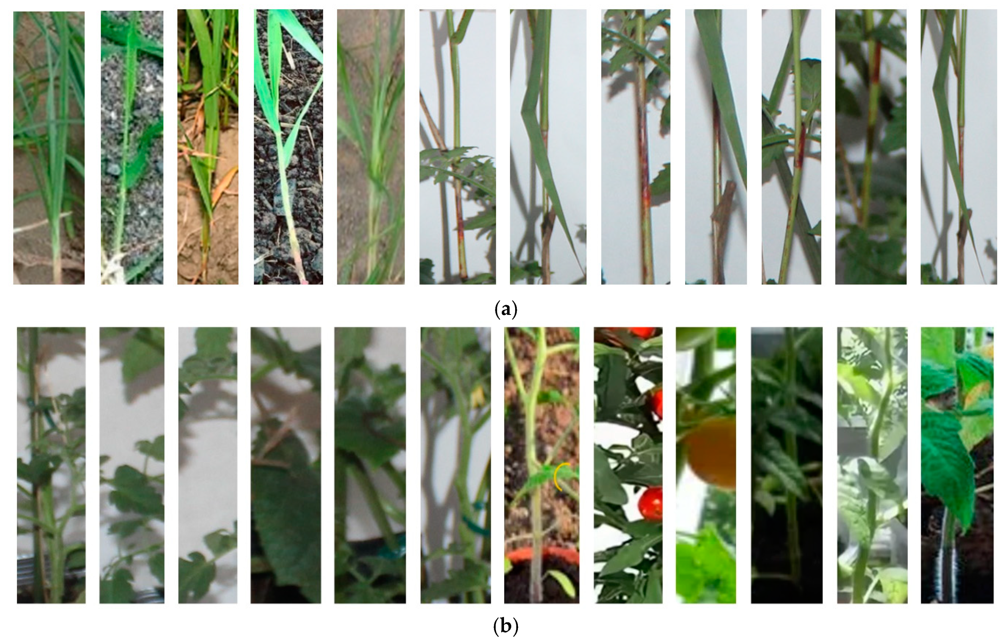
The Viola–Jones algorithm is a machine learning-based approach in which a cascade function is trained from many positive and negative images. The motive of images was selected visually placing the weed stalk in the center and including other weed parts in the image. It is then used to detect objects in other images in real time. Eight hundred positive examples of weeds and 1200 negative examples were used to train Haar cascade and SqueezeNet. The image size was 250 × 800 pixels (width × height). Eight hundred of the negative examples were images of tomato plants, and 400 images were images of other plants. Some positive and negative examples are shown in Figure 1.
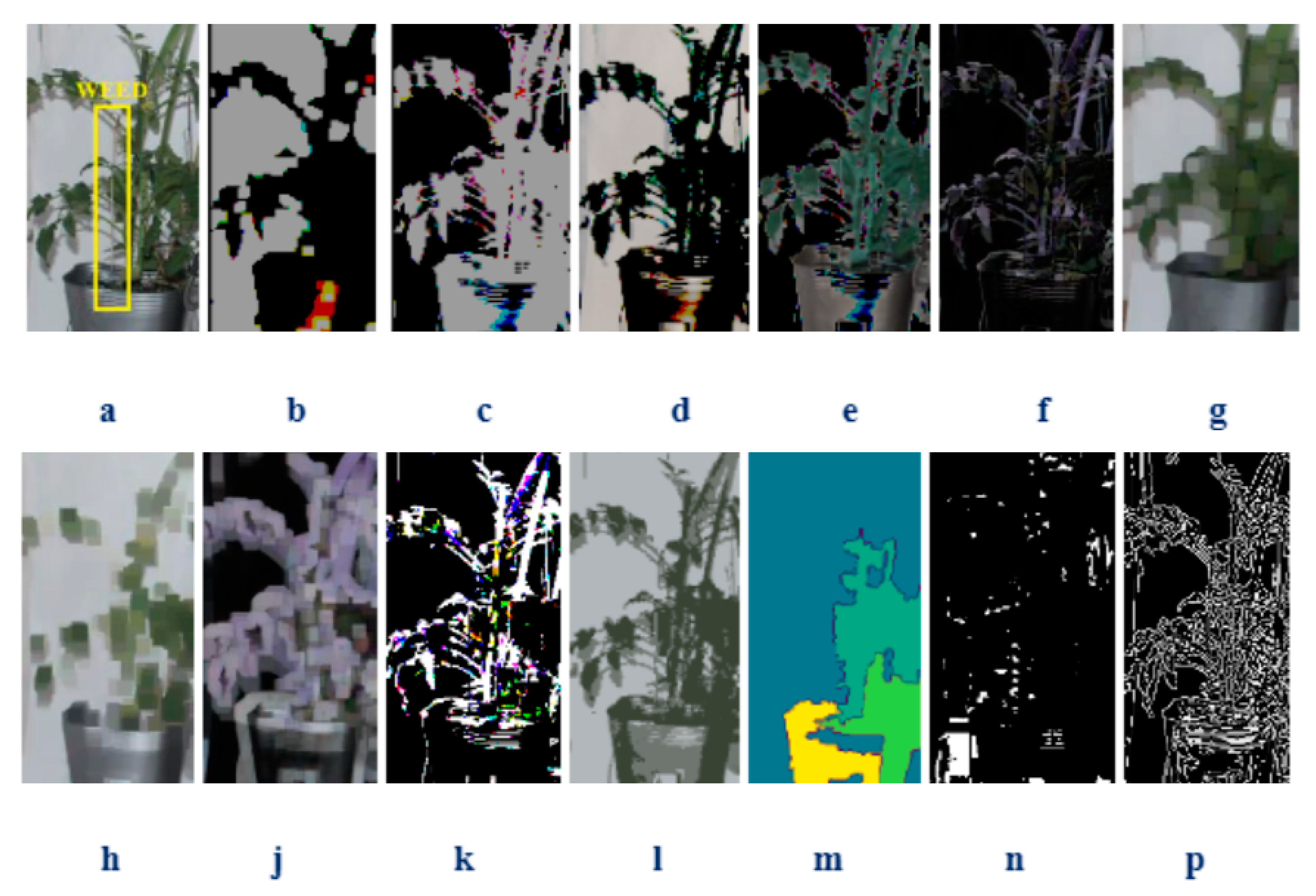
Image preprocessing was complicated by the fact that the weeds and crop were in a similar hue range, and, at the same time, close to each other. Therefore, we had to use 2000 images to train Haar cascades. OpenCV library functions were used for feature extraction (Figure 2). However, they did not result in a clear separation of crops and weeds, and, consequently, we decided using the images obtained from the camera without any transformations. Haar cascades were trained on plants located vertically in an angle of 90° from the surface.
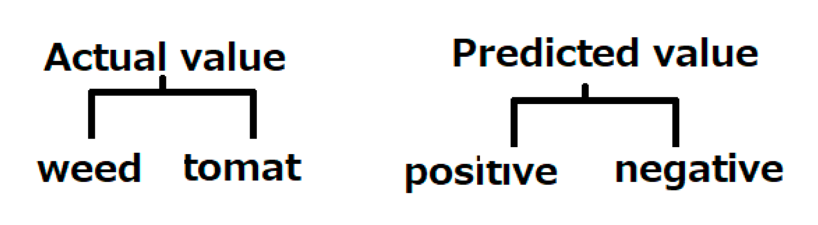
To assess the accuracy of the weed recognition, we used a confusion matrix. A confusion matrix is a table or chart that shows the prediction accuracy of a classifier for two or more classes (Figure 3). The classifier’s predictions are on the X-axis, and the result (accuracy) is on the Y-axis (see Results).
We tested our model for the weed recognition on 224 random images with weeds. The images were taken from the image collection prepared for checking the model. We used Python 3.6 and the standard library for visualization (seaborn and matplotlib) for displaying the confusion matrix (https://www.python.org/downloads/release/python-360/).
2.2. Method to Hit the Target
We applied OpenCV stereo vision functions to determine the distance to the objects, which made it possible to dispense with the use of distance measurement sensors (infrared sensors, sound locators or laser radars) [19,20,21,22]. We chose a camera that was compatibility with the Raspberry Pi–CSI connector, had a low price and a reasonable image quality. The Raspberry Pi and Sony IMX219 Exmor with the following specifications were used (Figure 4): Pi camera with Sensor type: Sony IMX219 Color CMOS 8MP; Sensor size: 3.674 × 2.760 mm (1/4 inch format); number of pixels: 3280 × 2464 (active pixels) 3296 × 2512 (total pixels); pixel size: 1.12 × 1.12 μm; lens: M12 customizable, telephoto fisheye lens; viewing angle: horizontal FOV 70 degrees; video: 1280 × 720 combined and cropped up to 60 fps; 1080P cropped to 30 fps; 1640 × 1232 full FOV binding mode, up to 30 fps; 3280 × 2464 full FOV, 0.1 to 15 fps; board size: 36 × 36 mm; IR sensitivity: built-in 650 nm IR cut filter, not sensitive to IR light; focal Length: 3.15 mm; aperture (F): 2.35.
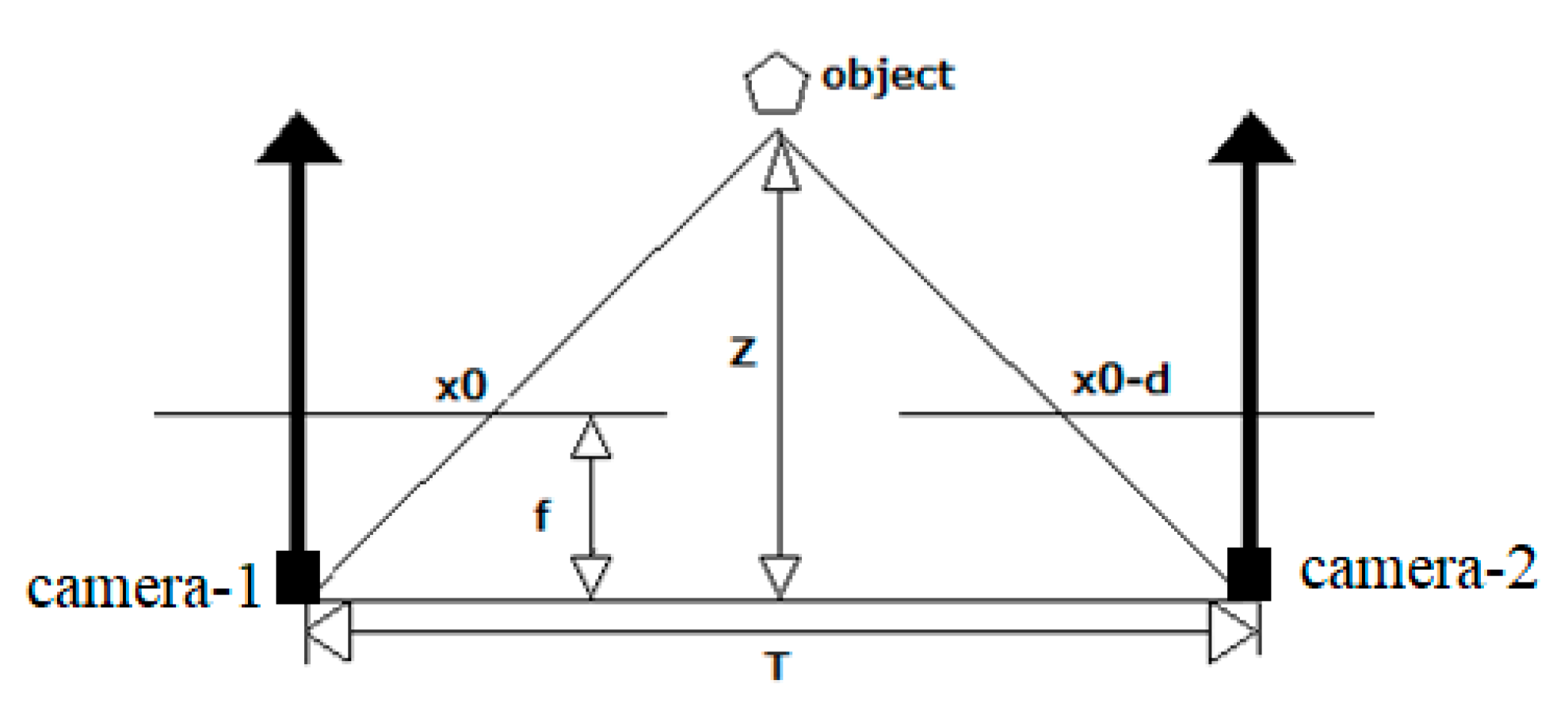
A depth map was built from a stereo pair. For each point in one image, a search was performed for its paired point in another image, and by a pair of corresponding points. We triangulated and determined the coordinates of their prototype in the three-dimensional space. Knowing the 3D coordinates of the pre-image, the depth was calculated as the distance to the camera plane.
The paired point was looked for on the epi-polar line. Accordingly, to simplify the search, images were aligned so that all the epi-polar lines are parallel to the sides of the image (usually horizontal). Moreover, the images are aligned so that for a point with coordinates (x0, y0) the corresponding epi-polar line is given by the equation x = x0; then, for each point, the corresponding paired point must be searched for in the same line in the image from the second camera. This process of aligning images is called rectification. Usually, rectification is performed by remapping the image and is combined with getting rid of distortions, but this was all done by the OpenCV library. We only had to calculate the distance between the cameras.
For simplicity and increased accuracy, special stereo cameras can be used—for example, the IMX219-83 8MP 3D Stereo Camera Module, which has a fixed and highly accurate position between the cameras. The distance between the cameras was calculated by the following formula:
where T is the distance between the cameras, d is a value called disparity/offset, Z is the distance to the target, and f is the focal length camera ratio (Figure 4).
(T − d)/(Z − f) = T/Z,
After the machine vision had confirmed the presence of a weed, a laser guidance system (Figure 5) converted the two-dimensional coordinates of the target into three-dimensional coordinates.
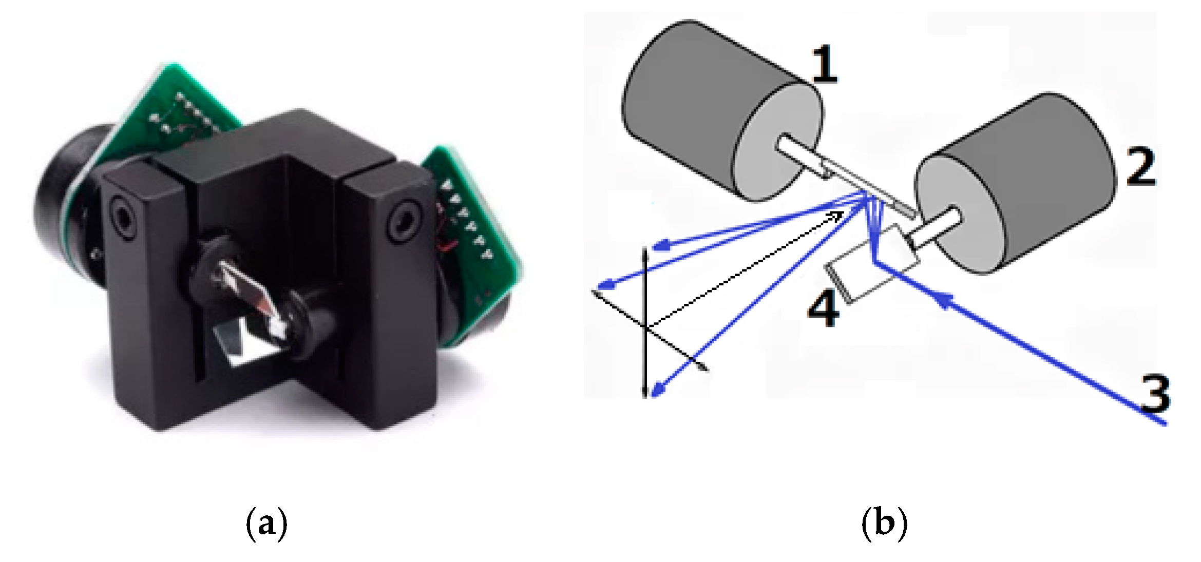
The laser guidance system consisted of a galvanometer (speed: 20 kpps) (Unbranded/Generic, style DMX Stage Ligh type: DHR814494, protocol for laser control: ILDA DB25) with two motors and two mirrors guiding the laser beam (Figure 5). This galvanometer is relative cheap (ca. $ 62). The device has two mirrors; one placed horizontally, and one placed vertically. Both mirrors were controlled by Raspberry PI that controlled the motor drivers. Drivers change the angle of the mirror.
The following expression describes the control of the positions of the galvanometer mirrors:
i is the time step, d is a value called disparity/offset, C is the three-dimensional coordinates of a point on the mirrors, n is the normal vectors of the units of the mirrors, and P is the target point on each mirror. It was necessary to calibrate the mirrors to get them to work correctly by using the potentiometer in the laser board before applying Formula (2).
2.3. The Laser System
Three lasers were tested: a 0.3 W laser (LBX Series, OXXIUS company, Lannion, France) with a wavelength of 405 nm, a 1 W laser (Blue Violet, TTL/PWM Focus Golden, Tgleiser, China) with a wavelength of 635 nm, and a 5 W laser (Jilin, MBL-W-457, Tgleiser, China) with a wavelength of 450 nm.
2.4. Decision Model for the Weed Control System
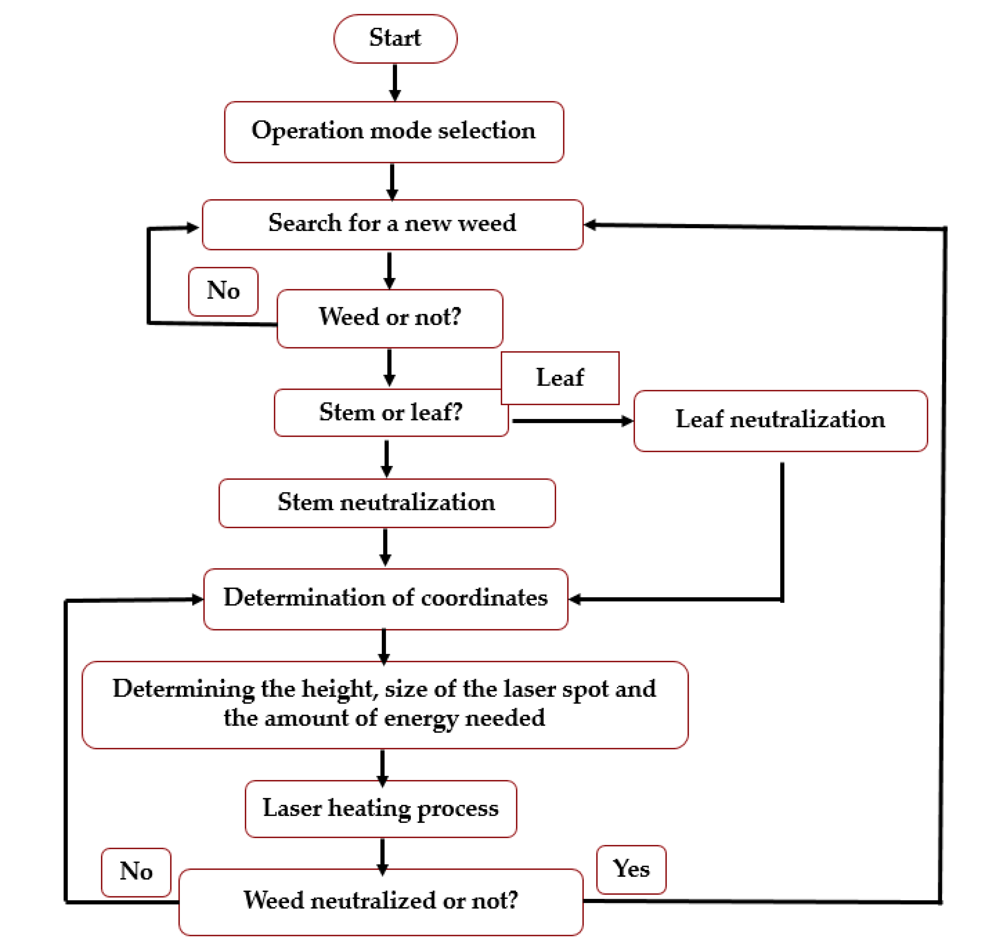
Figure 6 shows the decision model for the developed device. The Viola–Jones algorithm was used in the decision model.
2.5. Experimental Setup
Tomato plants were used as crops and couch grass (E. repens) as weeds. The plants were established in pots (10 cm Ø) with sphagnum and regularly watered ensuring that the plants had sufficient water during the experiments. Tomatoes were established from seeds and E. repens from rhizomes. No fertilizer was added to the pots during the experiment.
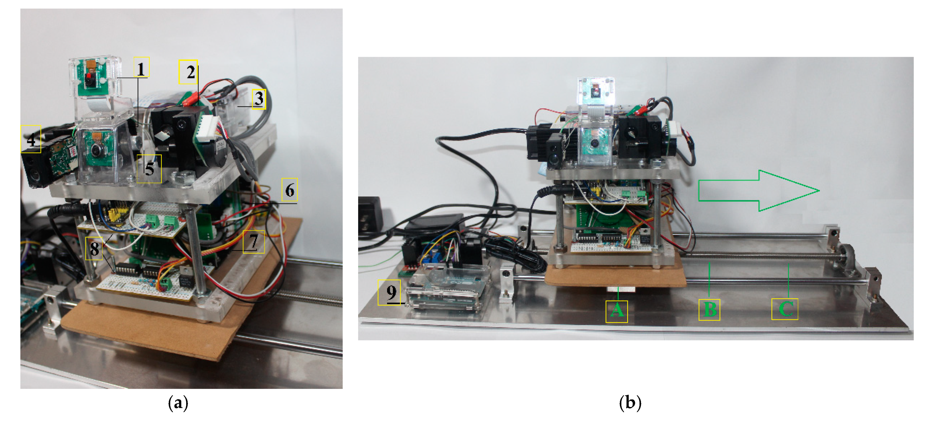
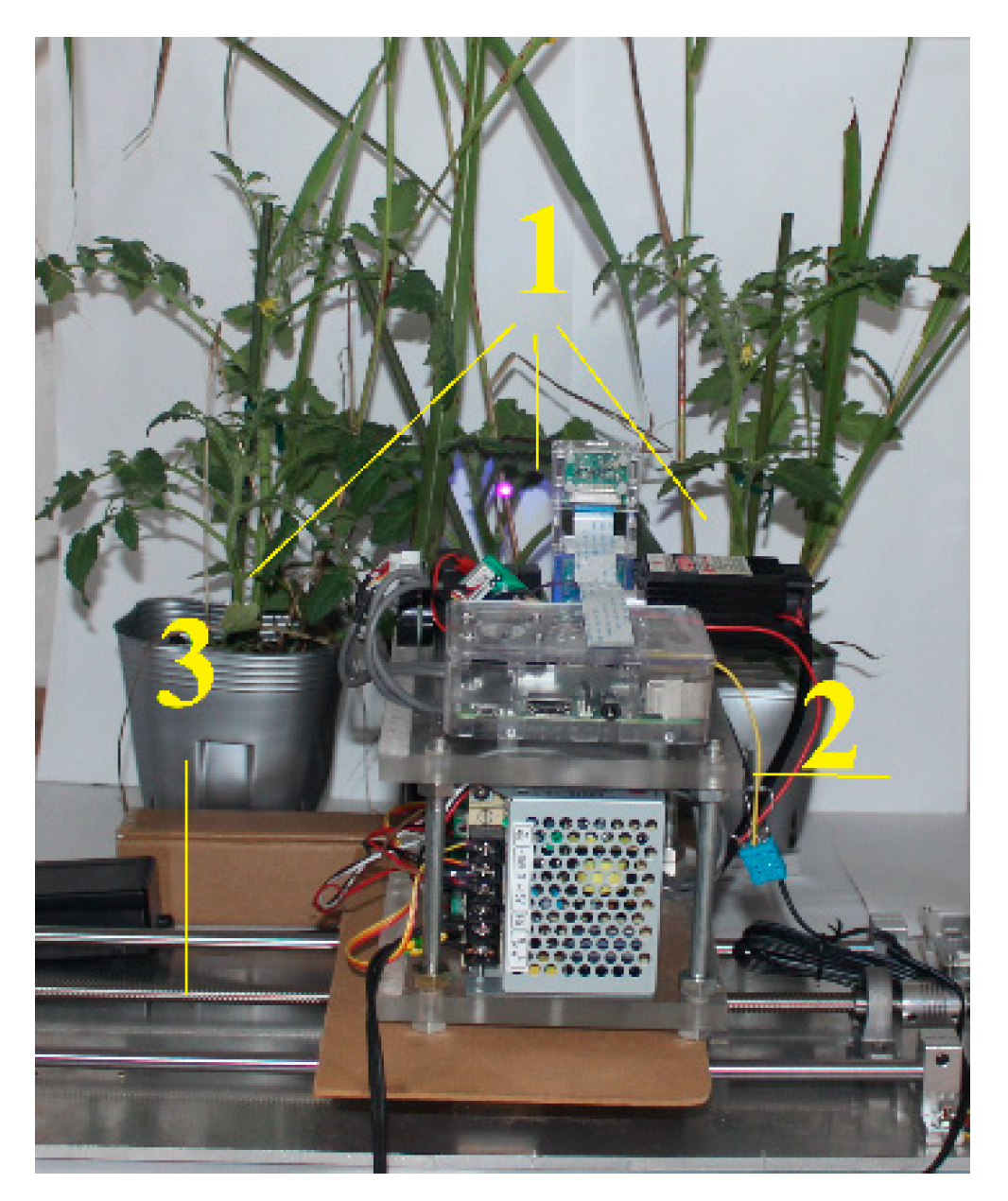
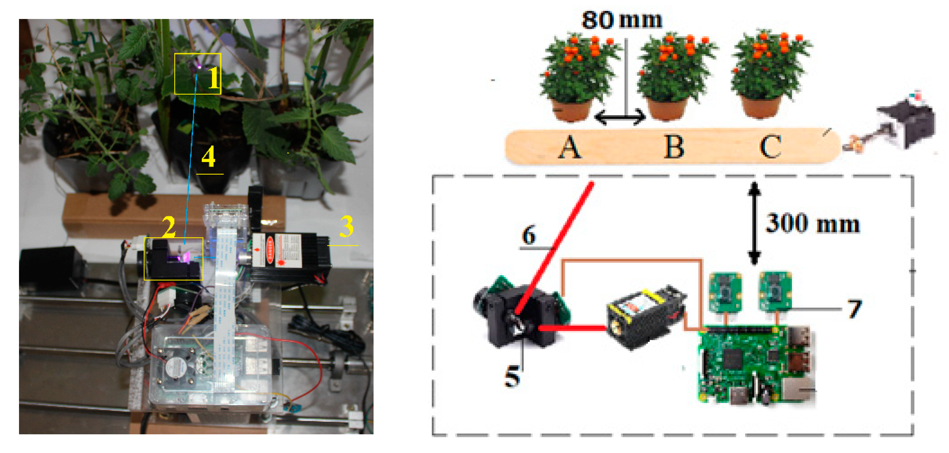
The device thermally damaged the stem of E. repens. After the stems of the weeds were hit, the plants either completely fell to the ground or bent. Figure 7 shows the prototype of the weed control device. The laser machine was able to move horizontally to mimic natural conditions. The experimental setup with E. repens between two tomato plants is shown in Figure 8.
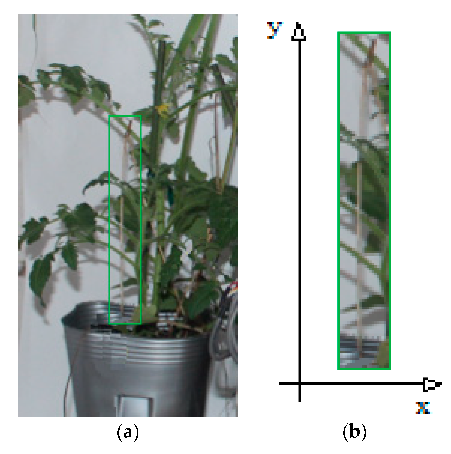
Figure 9 shows the process of determining the diameter of the stem of the weed.
It was not possible to determine the diameter of the stem from the Haar cascade as the diameter of the weed was determined together with the leaves because we used images of whole plants. Therefore, Haar cascades perceived the straw and leaves as one feature. The length of the weed was calculated with an error of 10% as the program knew the coordinates of the bounding rectangle for a detected object. Knowing the length of the weed, we could calculate its diameter. Figure 10 shows the path of the laser beam to the weed plant.
2.6. Experiments
2.6.1. The Relationship between Plant Lengths of E. repens and Plant Diameters
By using a caliper (Neiko 01407A; accuracy 0.02 mm), we manually measured the length and diameter of 75 E. repens plants for 80 days and described the relationship mathematically.
2.6.2. The Relationship between Required Energy to cut E. repens and Plant Diameters
We used the 75 plants with different diameter to study the necessary power to cut E. repens. We used a spot diameter of 0.55 mm for the laser beam.
2.6.3. The Relationship between Required Energy and the Diameter of the Laser Spot
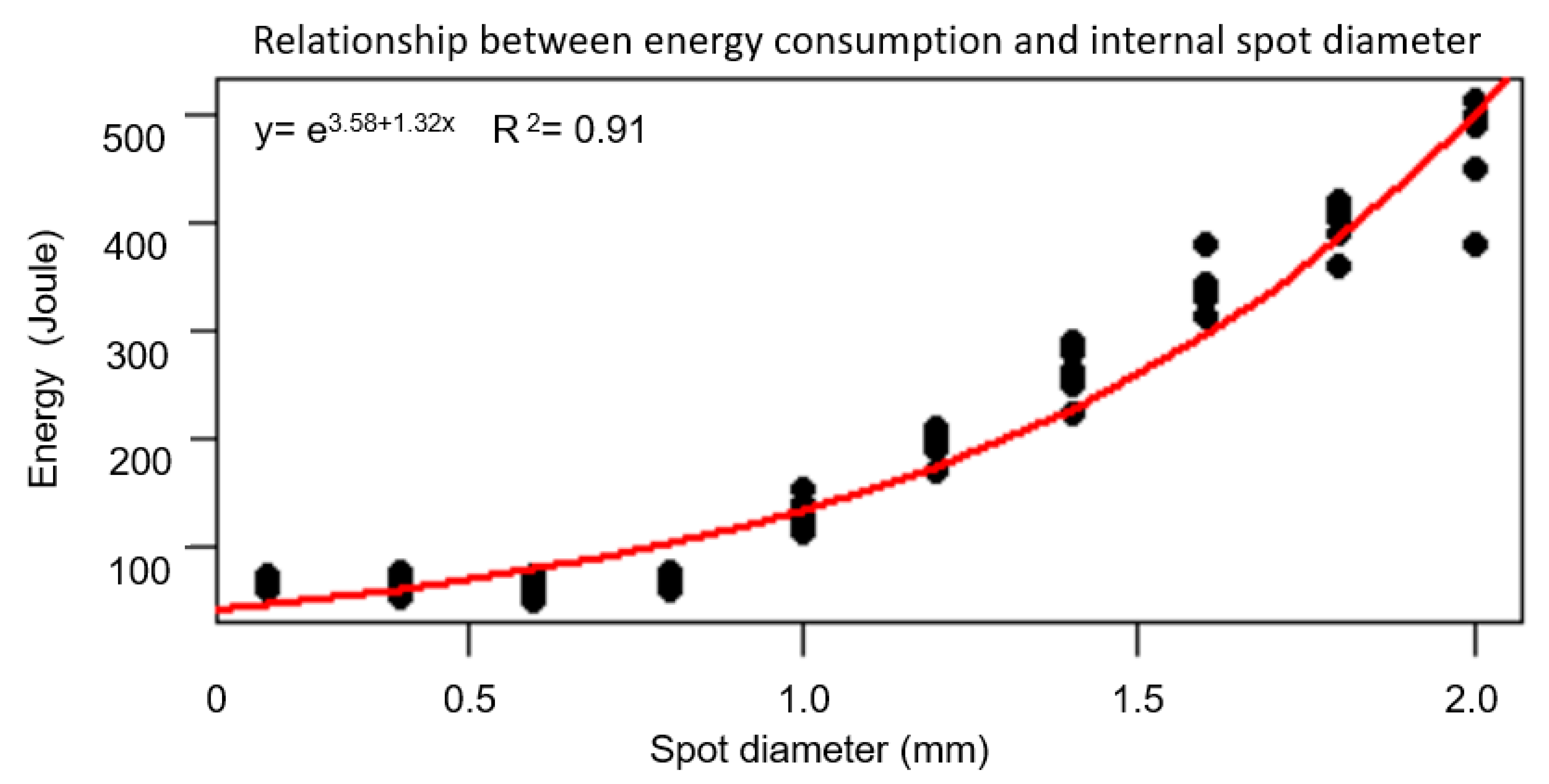
We estimated the mathematical relationship between energy consumption in Joule and the diameter (mm) of the spot of the laser beam for the 5 W laser. One second of exposure corresponded to 5 J.
2.6.4. The Relationship between Spot Diameter of the Laser Beam and the Effect of the Exposure
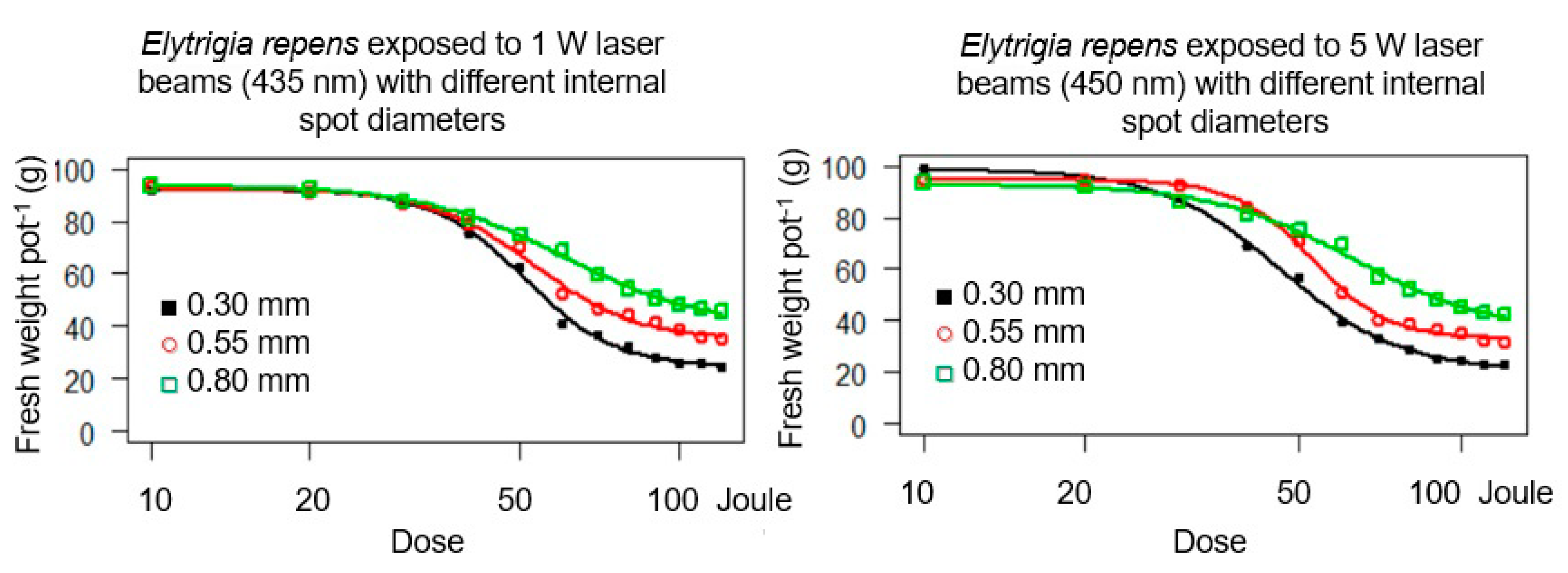
Dose-response experiments were conducted with two different lasers (1 W laser, 435 nm; 5 W laser, 450 nm) and with varying sizes of the focus spots of the laser beams on E. repens plants. We chose cheap lasers with the most common wavelength for the laser type.
The internal spot diameters were 0.30 mm, 0.55 mm, and 0.80 mm (±0.05 mm). Twelve dosages × 5 E. repens plants were used for each laser type. A dosage corresponded to the time (s) the plant was exposed to the laser beam. The plants were harvested 24 days after exposure, and the fresh weights were measured.
2.6.5. The Effect of the Three Lasers for Cutting Young Shoots of E. repens
Nine pots with three E. repens plants pot−1 (approximately 100 mm tall and 35 days old) were used for each treatment. The three lasers irradiated plants from a distance of 15−20 cm in the three pots. We placed the pots with weeds randomly between the tomatoes (Figure 8). The tomato plants had an age of 90 days and approximately 10 internodes. Each laser was fired approximately 200 times.
2.7. Data Analysis and Statistic
Linear regression was done using the GLM package in the open-source program R version 4.0.01 (The R Foundation for Statistical Computing, Vienna, Austria, http://R-project.org) to test whether plant length and diameter were linear related. Variance homogeneity was assessed by visual inspection of residual plots. The significance level was set to 0.05.
Statistical analysis of dose-response experiments was estimated using the add-on R package drc [22]. The effect of the irradiation on the fresh weight of weed plants was described by a four-parameter log-logistic model where the endpoint y depends on the dose x,
where y is the fresh weight of the plant (g pot−1), and x is the amount of energy applied (Joule). The parameter C denotes the lower limit of the curve. The parameter ED50 is the effective dose (energy in Joule) required to reduce the biomass by 50% between D and C. The parameter b is proportional to the slope at dose x equal to the parameter ED50.
The relationship between required energy and the diameter of laser spots was estimated using an exponential function using the lm R package.
3. Results
3.1. Detection of E. repens
The detection accuracy of E. repens depends on the number of datasets (images used in the Haar cascades) and how well the datasets reflect the real conditions. When using images collected under real conditions, we succeed with a detection accuracy of up to 88%. There were several reasons for failures: 1. The plants were not correctly detected 2. The machine vision did not detect E. repens. 3. The weed was detected, but its shapes were incorrectly determined. 4. Crop plant parts were defined as a weed.
We tested our model for weed recognition on 224 images with weeds; the visualization of the matrix is shown in the Figure 11.
The tracking accuracy was calculated to 80% based on the information from the confusion matrix (Figure 11) using the following formula:
where TP is a true positive decision; we predicted we found a weed and it was a weed. TN is a true negative decision; we predicted that this is not a tomato and it was true. P is the number of true results (95 + 84 = 179) and N is the number of false results (17 + 28 = 45). The false alarm factor: FPR = , where FP is a false positive decision (we predicted it was a weed, but it was not a weed) was estimated to 37%. The probability of detection = TP × 100/P, where TP is a true positive decision (we predicted we found a weed and it was a weed) was estimated to be 77%.
3.2. The Relationship between the Plant Lengths of E. repens and Plant Diameter
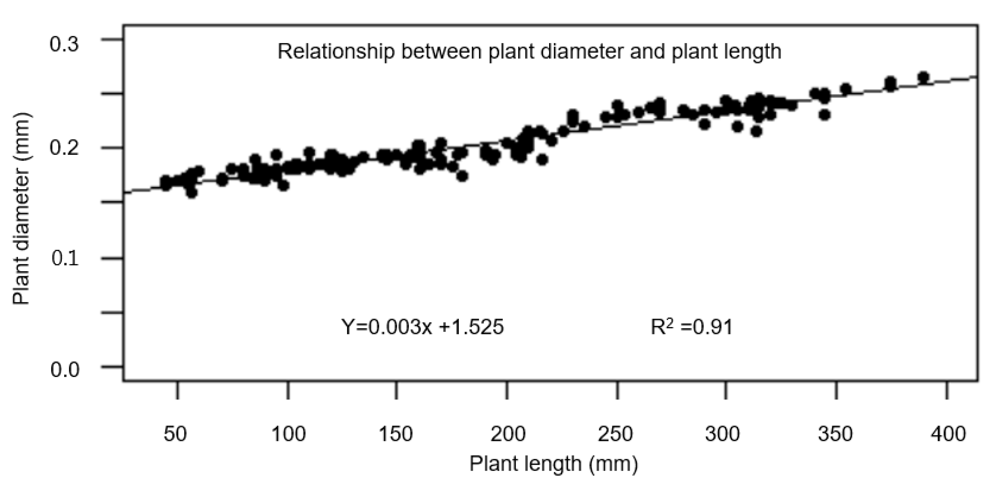
The relationship between plant lengths and plant diameters of 75 E. repens plants was described mathematically:
where y is the plant diameter (mm), and x is the length of the plant in mm (R2 = 0.91) (Figure 12).
y = 0.003x + 1.525
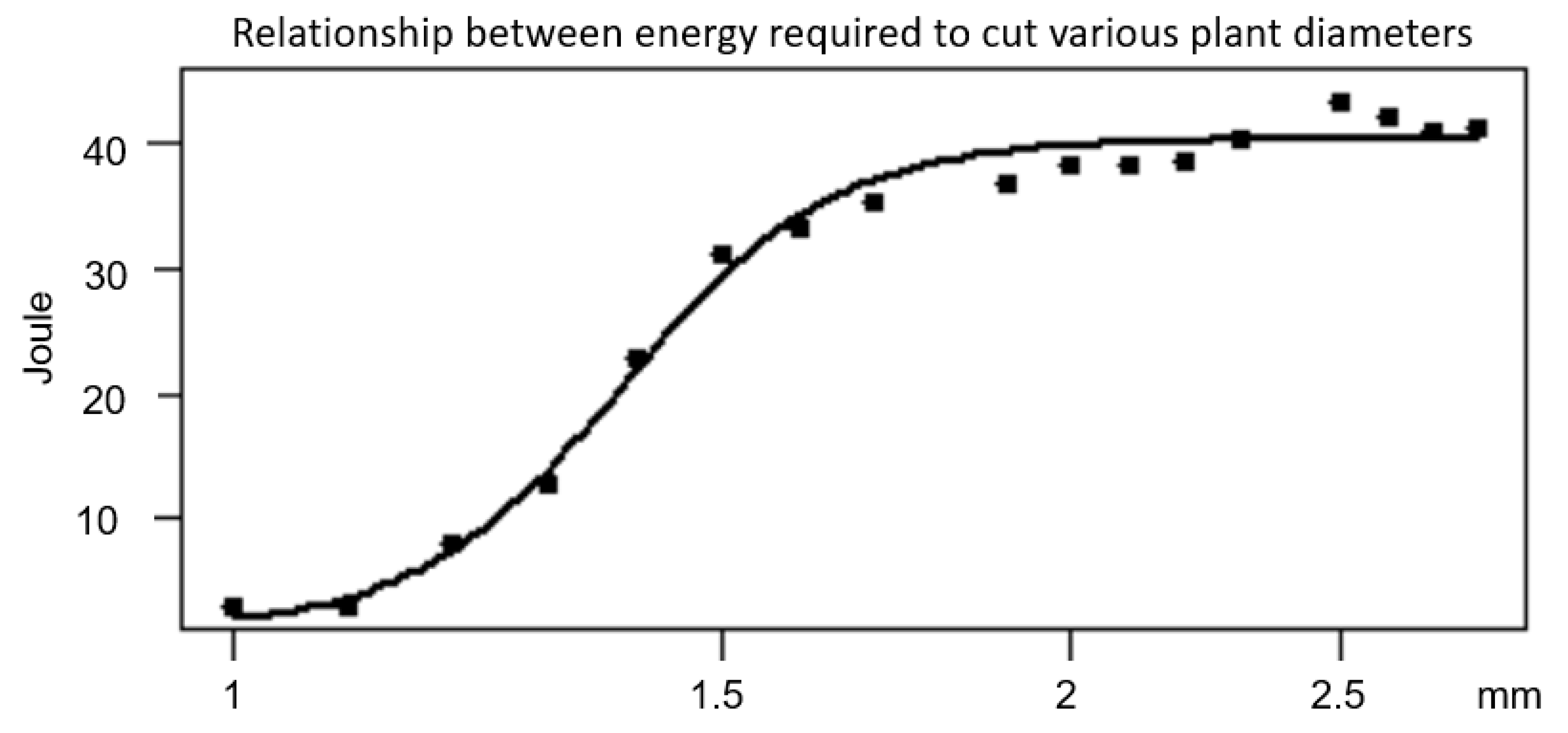
3.3. The Relationship between Required Energy to Cut E. repens and Straw Diameters
3.4. The Relationship between Required Energy and Laser Spot Diameter
The relationship between energy consumption (Joule) and the spot diameter of the laser beam (5 W laser) is shown in Figure 14.
3.5. The Relationship between Spot Diameter of the Laser Beam and the Effect of the Exposure
Figure 15 shows the dose-response curves with the two laser types (1 W laser, 5 W laser) where three intervals of spot sizes have been tested. The smaller the spot of the laser beam was, the better the weed control and utilization of energy. The parameters of the dose-response model are shown in Table 1. The models fitted the data very well (small SE-values) (Figure 13, Table 2).
Table 2 gives an overview of the experimental series with the three lasers. The most successful was the 5 W laser.
3.6. The Effect of the Three Lasers for Cutting Young Shoots of E. repens
Table 3 shows how efficient the system was. The 0.3 laser needed much more time to cut the shoots than the two other lasers, but it also harmed the tomato plants less. The 5 W laser was able to cut most E. repens shoots within 6 s. The weed detection system found about 86% of the E. repens plants.
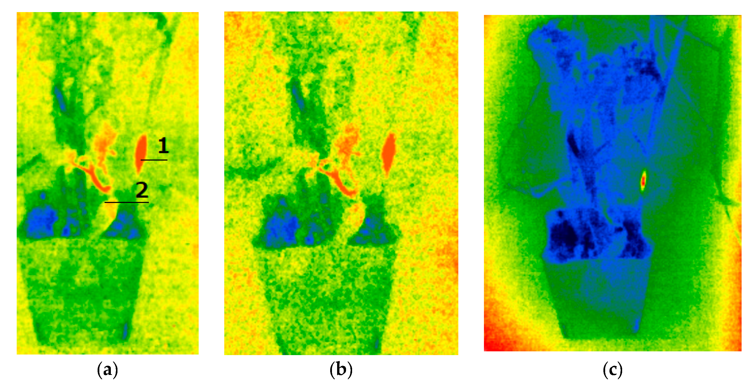
If the laser beam did not hit exactly in the middle of the E. repens shoot, the laser beam was split into two and therefore sometimes also hit and damaged the tomato plant (Figure 16).
The result of this phenomenon is shown on images taken by an infrared camera (Figure 17). Tomatoes were only exposed to laser irradiation one time on the same place during the test period. It is necessary to carry out additional research to understand how much the short-term irradiation may affect the tomatoes. However, we did not notice any detrimental effect of the short-term laser exposure on the tomato plants.
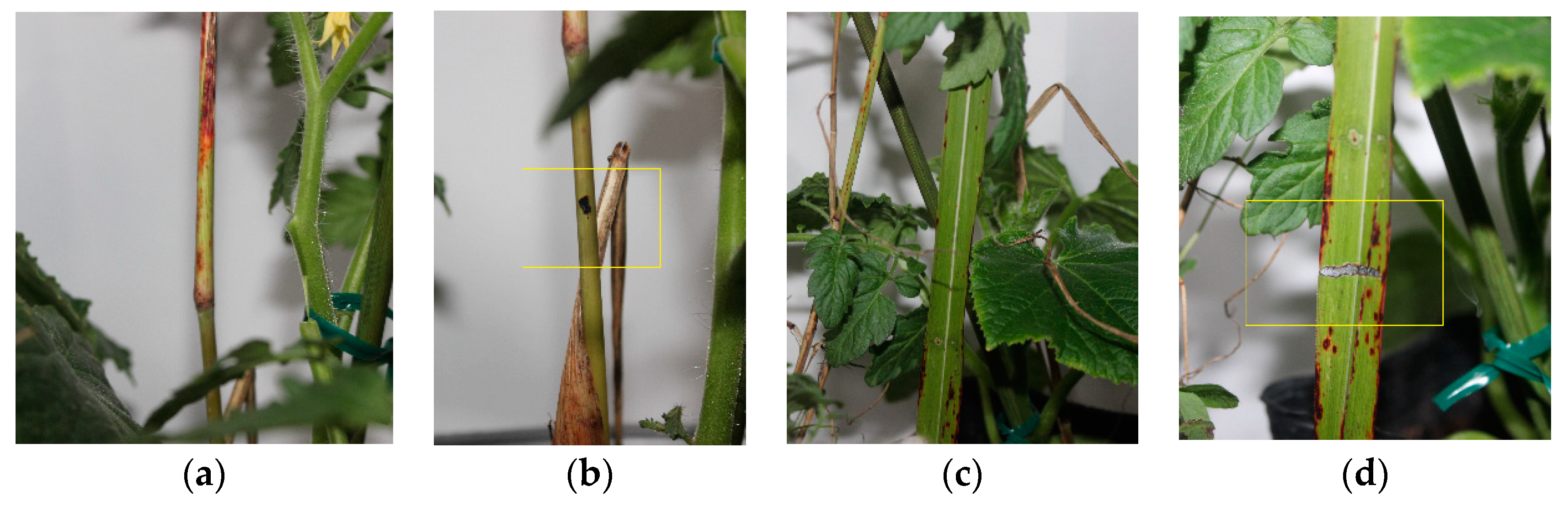
Figure 18 shows a straw and a leaf of E. repens before and after irradiation with a 1 W laser. A leaf cut was completed in less than a second but did not affect the plant much due to regrowth.
4. Discussion
There were some challenges with the image processing. Images of the subject in a real environment was needed to train the Haar cascades. The more alike the samples are to what we want to recognize, the better the results become. The tracking accuracy based on 224 test images was calculated to 80% and needs to be improved. Alternatively, the laser device may have to drive through the field more than one time. In the future, it is necessary to enlarge the matrix and consider several weeds and several plants. Many factors affect the precision of the detection of the weeds (e.g., lighting, background, and camera angle). Negative images (images without a weed) must be taken under the same conditions. Mounting a light source on the field equipment could ensure a constant and uniform lighting and thereby improve the precision of the weed detection.
Haar cascade is an edge detector. On that basis, a decision is made whether the cascade recognized the object in the image or not. To recognize the border between weed and crop in an image, there must be a color contrast between the weed and the crop.
We did not consider situations in which the weed and the tomatoes were tangled. Such cases require another approach. It is difficult to train the detecting of intertwined plants with Haar cascade, as components in the image that belong to weeds cannot be marked. The Haar cascade can only record the fact that weeds and crops have become tangled. A solution would be to use deep neural networks like Mask-RCNN, where objects manually can be marked for identification.
The laser beam has to hit the calculated coordinates of the target. The coordinates are given to the laser, and the galvanometer adjusts the laser so it hits the specific coordinate. We have achieved a galvanometer accuracy of 0.1 degrees, which allows hitting a target with an error of 1 mm at a distance of several meters.
It was sufficient to use a laser power of 1 W to cut E. repens plants with a diameter of more than 2 mm. However, a diameter of 2 mm requires a duration of 40 s making the system inefficient. For weeds with a diameter of more than 2 mm, a 5 W laser was necessary (Table 2). Therefore, we decided focusing on the 5 W laser.
If laser weeding is going to be used early in the growing season of the crop, laser weeding should take place when weeds only have developed a few leaves for monocots and 2−4 permanent leaves for dicots, and in that case, all weed stems would be less than 2 mm. In such cases, the laser should focus on leaves and meristems as the stems may be hidden by the leaves [15]. Small plants would be more sensitive to laser compared to the relatively large model plants we have used in this studied.
The laser spot diameter is an essential parameter [15] in relation to energy consumption. The larger spot diameter, the more energy is needed (Figure 13, Table 2). In the future, the machine vision of the system must be able to control the size of the spot diameter to operate efficiently. We changed the laser spot diameter by changing the distance between the laser and the galvanometer. In the future, we plan to use a laser with focus control.
When the laser spot decreases, the spot temperature increases linearly increasing the efficiency of the system. Focusing the laser requires a significant increase in the accuracy of the tracking system, video fixation, and stabilization of the laser position.
The diameter of the plant is related to the length (Figure 12) and age of the E. repens plant reflecting the mass fraction of the fluid content in the plant, which directly affects the amount of energy required to cut the grass (Figure 13). The experiments were conducted when plants were relatively large. Optimal weed control of E. repens is obtained just before or when the plants reach the compensation point at the 3−4 leaf stage [23]. After this stage, the net energy flow between the rhizomes and leaves changes, resulting in increased biomass of the rhizomes and therefore increasing ability to regrow.
Splitting of the laser beam was a problem that affected the crop. Sometimes, a part of the laser beam gets outside the view of the camera. In such cases, the system continues to work, and the calculated energy received by the weed became incorrect. Figure 16 shows an example where the laser beam is located both on the E. repens plant and on the crops. By using a laser with a power less than 1 W, the divided energy was insufficient to damage crop plants within a short time. A 1 W laser would probably we sufficient to control small weed plants.
There is a need to analyze the influence of the laser beam on the weed after irradiation. If the color of the hit point on the weed is more or less unchanged, the damage has not been sufficient, and the plant will be able to recover (Figure 17 and Figure 18).
The number of images used for training the algorithm needs to be increased for reducing the error of identification of weeds and crop. For example, the laser could be programmed to irradiate only if there is a 90% probability that the plant is a weed to avoid harming the crop with the laser (Figure 16 and Figure 17). However, that will reduce weeding efficiency.
Figure 18b presents the result of an incorrect calculation of the necessary energy to cut the weed because of the wrong estimation of the plant diameter by the machine vision system resulting in insufficient damage. Figure 18c shows a damaged leaf. However, the damaged leaf did not prevent the plant from recovering, and therefore we decided to focus on irradiation of the straws.
Figure 18 showed that black spots present on the weed were not a good indicator for significant damage to the plant. The best sign is a physical rift of the stem for visual confirmation.
The next step will be to conduct experiments in a field with a crop by installing the equipment on a tractor. It will be necessary to upgrade the installation and place it in a protected IP54 enclosure. The Raspberry Pi 3 Model B+ computer will be replaced with a STM32 microcontroller (STMicroelectronics, Genève, Schweiz). A STM32 has an X-CUBE-AI - AI - expansion pack for STM32CubeMX. This extension can work with various deep learning environments such as Caffe, Keras, TensorFlow, Caffe, ConvNetJs, which makes it possible to train with a stationary computer with a Graphics Processing Unit (GPU). After this integration, it can be used to optimize the library for the 32-bit STM32 microcontroller. A telephoto will be connected to the pi cam lens to increase the weed control area, and a camera will be connected to the servomotor to move along the z-axis.
In order to develop a low-cost laser weeding system, we used a Raspberry Pi camera 8 MP (price <20 dollars) equipped with an eight-megapixel (8 MP) Sony IMX219 Exmor sensor, which could capture, record, and stream video in 1080 p. The maximum image resolution reached 3280 × 2464 pixels. The system could be improved significantly by using a better camera with a resolution of more than 8 MP with autofocus covering a large infested area.
In addition, it is necessary to work out protective measures (e.g., shields) to avoid unwanted impact on persons, material and the surrounding environment.
Although several groups have studied the effect of laser beams on weeds e.g., [13,14,15] only a few have developed an automatic device for controlling weeds with laser beams. Xiong et al. [16] developed a robot equipped with machine vision and laser pointers. The robot identified weeds in indoor environments, and the lasers irradiated the weeds at the cotyledon stage. Our system works in a much more complex system with large grass weeds and crop plants partly covering each other. Therefore, the identification of weeds and crops became much more complicated, and the system requires a huge amount of images to develop a machine vision with high precision. In the future, we will focus on controlling small weed plants to reduce the energy consumption and initiate weed control early in the growing season before the competition between the crop and the weeds starts. We consider that developing a prototype of a robot for controlling emerging weeds with laser beams in row crops like maize, sugar beets, and horticultural crops would be an obtainable goal within the next three years.
5. Conclusions
A laser weeding system based on rather cheap equipment was created. Machine vision was used to find tall Elytrigia repens plants among tomato plants in a controlled environment. Image processing was complicated by the fact that the weeds and crop were in a similar hue range, and close to each other. We used untransformed images obtained from the RGB camera, as transformations did not improve the separation of weeds and crop. Haar cascades were trained on E. repens located vertically, and three lasers were tested to cut and control E. repens from the side. We found a linear relationship between plant lengths and plant diameters, which was used to estimate the spot diameter necessary to cut an E. repens shoot. The relationship between energy consumption (Joule) for cutting E. repens shoots and shoot diameters followed a S-shaped function, while the relationship between energy consumption (Joule) and the spot diameter of the laser beam (5 W laser) followed an exponential function. The relationship between spot diameter of the laser beam and the effect of the exposure also followed and S-shaped curve. The smaller the internal spot diameter of the laser beam, the better control of the weed. The 5 W laser turned out to be the most promising to cut large E. repens plants, (shoot diameter >2 mm), but it also increased the risk of damaging the crop. A 1 W or 3 W laser would probably be sufficient to control small weed plants.
Author Contributions
I.R. designed the concept, conducted the experiments and wrote the research protocol. C.A. did the statistical analysis of data and wrote the manuscript. Both authors edited and accepted the final paper. All authors have read and agreed to the published version of the manuscript.
Funding
This research was funded by South Ural State University, Russia, the University of Copenhagen, Denmark, and the EU–project WeLASER “Sustainable Weed Management in Agriculture with Laser-Based Autonomous Tools,” Grant agreement ID: 101000256 funded under H2020-EU.3.2.1.1.
Acknowledgments
We thank Marat Zhanikeev, Tokyo University of Science, for comments and recommendations concerning setup of the laser system.
Conflicts of Interest
The authors declare no conflict of interest. The funders had no role in the design of the study; in the collection, analyses or interpretation of data; in the writing of the manuscript; or in the decision to publish the results.
References
- FAO. AGP—Weeds. 2017. Available online: http://www.fao.org/agriculture/crops/thematicsitemap/theme/biodiversity/weeds/en/ (accessed on 7 July 2020).
- Heap, I. Herbicide resistant weeds. In Integrated Weed Management; Pimental, D., Peshin, E., Eds.; Springer: Dordrecht, The Netherlands, 2014; pp. 281–301. [Google Scholar]
- Andreasen, C.; Streibig, J.C. Evaluation of changes in weed flora in arable fields of Nordic countries—Based on Danish long-term surveys. Weed Res. 2011, 51, 214–226. [Google Scholar] [CrossRef]
- Chauvel, B.; Guillemin, J.-P.; Gasquez, J.; Gauvrit, C. History of chemical weeding from 1944 to 2011 in France: Changes and evolution of herbicide molecules. Crop. Prot. 2012, 42, 220–223. [Google Scholar] [CrossRef]
- Duke, S. Why have no new herbicide modes of action appeared in recent years? Pest. Manag. Sci. 2011, 68, 505–512. [Google Scholar] [CrossRef] [PubMed] [Green Version]
- Funk, C.; Kennedy, B. The New Food Fights: U.S. Public Divides Over Food Science; Differing Views on Benefits and Risks of Organic Foods, GMOs as Americans Report Higher Priority for Healthy Eating; Pew Research Center: Washington DC, USA, 2016. [Google Scholar]
- Liebmann, M.; Dyck, E. Crop rotation and intercropping strategies for weed management. Ecol. Appl. 1993, 3, 92–122. [Google Scholar] [CrossRef] [PubMed]
- Cloutier, D.; Leblanc, M.L. Mechanical Weed Control in Agriculture. In Physical Control Methods in Plant Protection, 1st ed.; Vincent, C., Panneton, B., Fleurat-Lessard, F., Eds.; Springer: Berlin/Heidelberg, Germany, 2001; pp. 191–204. [Google Scholar]
- Sivesind, E.; Leblanc, M.; Cloutier, D.; Siguin, P.; Stewart, K. Weed response to flame weeding at different development stages. Weed Res. 2009, 23, 438–443. [Google Scholar] [CrossRef]
- Andreasen, C.; Bitarafan, Z.; Fenselau, J.; Glasner, C. Exploiting waste heat from combine harvesters to damage harvested weed seeds and reduce weed infestation. Agriculture 2018, 8, 42. [Google Scholar] [CrossRef] [Green Version]
- Bitarafan, Z.; Andreasen, C. Harvest Weed Seed Control: Seed production and retention of Fallopia convolvulus, Sinapis arvensis, Spergula arvensis and Stellaria media at spring oat maturity. Agronomy 2020, 10, 42. [Google Scholar] [CrossRef] [Green Version]
- Heisel, T.; Schou, J.; Andreasen, C.; Christensen, S. Using laser to cut and measure thickness of Beta vulgaris L. and Solanum nigrum L. stems. Weed Res. 2002, 42, 242–248. [Google Scholar] [CrossRef]
- Heisel, T.; Schou, J.; Christensen, S.; Andreasen, C. Cutting weeds with CO2 laser. Weed Res. 2001, 41, 19–29. [Google Scholar] [CrossRef]
- Marx, C.; Barcikowski, S.; Hustedt, M.; Haferkamp, H.; Rath, T. Design and application of a weed damage model for laser-based weed control. Biosyst. Eng. 2012, 113, 148–157. [Google Scholar] [CrossRef]
- Mathiassen, K.; Bak, T.; Christensen, S.; Kudsk, P. The effect of laser treatment as a weed control method. Biosyst. Eng. 2006, 95, 497–505. [Google Scholar] [CrossRef] [Green Version]
- Xiong, Y.; Ge, Y.; Liang, Y.; Blackmore, S. Development of a prototype robot and fast path-planning algorithm for static laser weeding. Comput. Electron. Agric. 2017, 142, 494–503. [Google Scholar] [CrossRef]
- Viola, P.; Jones, M. Robust real-time face detection. Int. J. Comput. Vis. 2004, 57, 137–154. [Google Scholar] [CrossRef]
- Ganesh, A. Deep Learning Reading Group: SqueeszeNet. 2016. Available online: https://www.kdnuggets.com/2016/09/deep-learning-reading-group-squeezenet.html (accessed on 20 October 2020).
- Wrzesień, M.; Treder, W.; Klamkowski, K.; Rudnicki, W. Prediction of the apple scab using machine learning and simple weather stations. Comput. Electron. Agric. 2019, 161, 252–259. [Google Scholar] [CrossRef]
- Dorina, B.; Pierre-Benoît, J. Modelling world agriculture as a learning machine? From mainstream models to Agribiom 1.0. Land Use Policy 2009, 96, 103624. [Google Scholar] [CrossRef]
- Suchithra, M.; Maya, L. Improving the prediction accuracy of soil nutrient classification by optimizing extreme learning machine parameters. Inf. Process. Agric. 2019, 7, 72–82. [Google Scholar] [CrossRef]
- Ritz, C.; Streibig, J.C. Bioassay analysis using R. J. Stat. Softw. 2005, 12, 5. [Google Scholar] [CrossRef] [Green Version]
- Håkansson, S. Weeds and Weed Management on Arable Land. An. Ecological Approach, 1st ed.; Cabi: Wallingford, UK, 2003; p. 247. [Google Scholar]
Figure 1.
Images used to train Haar cascades. (a) Examples of images with E. repens (positive image). (b) Examples of images with other plants (negative images).
Figure 1.
Images used to train Haar cascades. (a) Examples of images with E. repens (positive image). (b) Examples of images with other plants (negative images).

Figure 2.
Examples of feature extraction: (a) received image with weed and tomato, (b) image thresholding by cv2.threshold (img,127,155,cv2.THRESH_BINARY), (c) image thresholding by cv2.threshold(img,127,155,cv2.THRESH_BINARY_INV), (d) image thresholding by cv2.threshold(img,127,155,cv2.THRESH_TOZERO), (e) image thresholding by cv2.threshold(img,127,155,cv2.THRESH_TOZERO_INV), (f) morphological transformations by cv2.morphologyEx(img, cv2.MORPH_BLACKHAT, kernel1), (g) morphological transformations by cv2.morphologyEx(img, cv2.MORPH_OPEN, kernel2), (h) morphological transformations by cv2.morphologyEx(img, cv2.MORPH_CLOSE, kernel2), (j) morphological transformations by cv2.morphologyEx(img, cv2.MORPH_GRADIENT, kernel2), (k) flood fill by cv2.floodFill(im_floodfill, mask, (0, 0), 255), (l) segmentation by cv2.kmeans(pixel_values), (l) none, criteria, 10. cv2.KMEANS_RANDOM_CENTERS), (m) distance transform by cv2.distanceTransform(opening,cv2.DIST_L2,5), (n) color detection by cv2.inRange(hsv, h_min, h_max), (p) edge detection cv2.Canny(img,100,200).

Figure 3.
Illustration of information necessary to construct a confusion matrix.

Figure 4.
The positions of the cameras to determine the distance to the object: d is a value called disparity/offset, T is the distance between the cameras, Z is the distance to the object, and f is the focal length camera ratio.
Figure 4.
The positions of the cameras to determine the distance to the object: d is a value called disparity/offset, T is the distance between the cameras, Z is the distance to the object, and f is the focal length camera ratio.

Figure 5.
Galvanometer operating principle. (a) Photo of a galvanometer; (b) the principle of operation. 1 and 2 are motors, 3 is the laser beam, and 4 are mirrors for laser reflection.
Figure 5.
Galvanometer operating principle. (a) Photo of a galvanometer; (b) the principle of operation. 1 and 2 are motors, 3 is the laser beam, and 4 are mirrors for laser reflection.

Figure 6.
A decision model for the weed control device.

Figure 7.
The prototype of the weed control device. (a) 1. Pointing to the cameras; 2. galvanometer; 3. Raspberry computer; 4. laser rangefinder; 5. laser; 6. power supply; 7. motor drivers, 8. electronic signal processing board, 9. Arduino board to control the position of the laser setup. (b) A, B, and C show the location of the crops.

Figure 8.
The experimental setup with E. repens between tomato plants. 1. Elytrigia repens plant; 2. the laser installation; 3. the device was allowing the laser to move horizontally.
Figure 8.
The experimental setup with E. repens between tomato plants. 1. Elytrigia repens plant; 2. the laser installation; 3. the device was allowing the laser to move horizontally.

Figure 9.
Determination of the diameter of the stem of the weed. (a) Identification of the weed; (b) calculation of the length of the weed.
Figure 9.
Determination of the diameter of the stem of the weed. (a) Identification of the weed; (b) calculation of the length of the weed.

Figure 10.
The experimental set up. 1. Focusing the laser beam; 2. mirrors from the galvanometer; 3. the laser; 4. laser beam; 5. galvanometer; 6. schematic image of the laser beam; 7. cameras.
Figure 10.
The experimental set up. 1. Focusing the laser beam; 2. mirrors from the galvanometer; 3. the laser; 4. laser beam; 5. galvanometer; 6. schematic image of the laser beam; 7. cameras.

Figure 11.
A confusion matrix showing the prediction accuracy of a classifier for two or more classes. The classifier’s predictions are on the X-axis and the result (accuracy) is on the Y-axis. TP is a true positive decision; we predicted we found a weed and it was a weed. FP is a false positive decision; we predicted it was a weed, but it was not a weed. FN is a false negative decision; we predicted it was not tomato and it was not true. TN is a true negative decision; we predicted that this is not a tomato and it was true.

Figure 12.
The relationship between plant diameters (mm) of E. repens and plant lengths (mm).

Figure 13.
The relationship between energy consumption (Joule) for cutting plants of E. repens with various shoot diameters (mm) (5 W laser).
Figure 13.
The relationship between energy consumption (Joule) for cutting plants of E. repens with various shoot diameters (mm) (5 W laser).

Figure 14.
The relationship between the energy consumption and the diameter of the laser spot (mm). The larger the laser spot diameter has to be to damage a shoot of E. repens, the more energy is needed.
Figure 14.
The relationship between the energy consumption and the diameter of the laser spot (mm). The larger the laser spot diameter has to be to damage a shoot of E. repens, the more energy is needed.

Figure 15.
Dose-response curves. (a) E. repens plants were exposed to a 1 W laser (435 nm) beams and (b) to a 5 W laser (450 nm) beams. Three diameters (+/− 0.05 mm) of the internal spot of the laser beams were used: ■ 0.30 mm; ○ 0.55 mm; □ 0.80 mm. The plants were harvest 40 days after laser exposure.

Figure 16.
Sometimes under the operation, the laser beam was split into two beams as the violet spots show, resulting in damage of crop plants.
Figure 16.
Sometimes under the operation, the laser beam was split into two beams as the violet spots show, resulting in damage of crop plants.

Figure 17.
Infrared images of the result of a divided laser beam. The three images were taken with 10-s intervals. (a) This image was taken immediately after the treatment. 1. The spot where the straw of the E. repens was hit. 2. The damage tomato plant: (b) image taken 10 s after the first image; (c) image taken 20 s after the first image.

Figure 18.
Elytrigia repens plant before and after irradiation with a 1 W laser for 0.5 s. (a) The straw before the irradiation; (b) the straw after the irradiation; (c) the leaf of E. repens before the irradiation and (d) after the irradiation.
Figure 18.
Elytrigia repens plant before and after irradiation with a 1 W laser for 0.5 s. (a) The straw before the irradiation; (b) the straw after the irradiation; (c) the leaf of E. repens before the irradiation and (d) after the irradiation.


Table 1.
Estimated parameters and standard errors (SE) of the dose-response models (model 3) for experiments with a 5 W laser showing the relationship between energy consumption (Joule) for cutting plants E. repens with various shoot diameters (mm) corresponding to the curve in Figure 13. The parameter ED50 is the effective dose (energy in Joule) required reducing the biomass by 50% between D and C. The parameter b is proportional to the slope at dose x equal to the parameter ED50.
| Laser Type | Relative Slope | Lower Limit (Joule) | Upper Limit (Joule) | ED50 (mm) |
|---|---|---|---|---|
| b | C | D | ||
| 5 W (450 nm) | 11.61 (1.17) | 1.19 (1.17) | 40.20 (0.43) | 1.38 (0.01) |
Table 2.
Estimated parameter and standard errors (SE) of the dose-response models (model 3) for experiments with two laser types and three intervals of internal laser spot diameter corresponding to the curves in Figure 15. The parameter ED50 is the effective dose (energy in Joule) required to reduce the biomass by 50% between D and C. The parameter b is proportional to the slope at dose x equal to the parameter ED50.
| Laser Type | Laser Spot Diameter | Relative Slope | Lower Limit (g pot−1) | Upper limit (g pot−1) | ED50 (Joule) |
|---|---|---|---|---|---|
| b | C | D | |||
| 1 W (430 nm) | 0.30 mm | 5.0 (0.4) | 24.3 (1.3) | 92.0 (1.2) | 51.0 (0.9) |
| 1 W (430 nm) | 0.55 mm | 4.4 (0.5) | 34.6 (1.6) | 92.4 (1.3) | 53.1 (1.3) |
| 1 W (430 nm) | 0.80 mm | 3.2 (0.4) | 39.4 (2.7) | 93.6 (1.2) | 60.6 (2.3) |
| 5 W (450 nm) | 0.30 mm | 3.9 (0.4) | 20.3 (2.0) | 98.6 (2.0) | 46.4 (1.2) |
| 5 W (450 nm) | 0.55 mm | 6.2 (0.7) | 32.7 (1.2) | 94.6 (1.2) | 53.0 (0.9) |
| 5 W (450 nm) | 0.80 mm | 3.3 (0.4) | 35.4 (2.7) | 92.7 (1.1) | 62.9 (2.1) |
Table 3.
The effect of the laser system using three different lasers for cutting 35-day-old shoots of E. repens (less than 100 mm tall). Each laser was fired approximately 200 times. Some tomatoes were also hit and left with traces on the leaves but did not kill the plants.
Table 3.
The effect of the laser system using three different lasers for cutting 35-day-old shoots of E. repens (less than 100 mm tall). Each laser was fired approximately 200 times. Some tomatoes were also hit and left with traces on the leaves but did not kill the plants.
| No. | Laser Power W | Laser Spot Mm | Distance cm | Damaged Tomatoes % | Laser Time s | Energy J | Average Detection % | A Complete Cut of Straw % |
|---|---|---|---|---|---|---|---|---|
| 1 | 0.3 | 0.30 | 15−20 | 0.5 | 76 | 23 | 85 | 84 |
| 2 | 1 | 0.55 | 15−20 | 1.5 | 23 | 23 | 88 | 85 |
| 3 | 5 | 0.80 | 15−20 | 7 | 6 | 35 | 85 | 97 |
Publisher’s Note: MDPI stays neutral with regard to jurisdictional claims in published maps and institutional affiliations. |
© 2020 by the authors. Licensee MDPI, Basel, Switzerland. This article is an open access article distributed under the terms and conditions of the Creative Commons Attribution (CC BY) license (http://creativecommons.org/licenses/by/4.0/).
Share and Cite
MDPI and ACS Style
Rakhmatulin, I.; Andreasen, C. A Concept of a Compact and Inexpensive Device for Controlling Weeds with Laser Beams. Agronomy 2020, 10, 1616. https://0-doi-org.brum.beds.ac.uk/10.3390/agronomy10101616
AMA Style
Rakhmatulin I, Andreasen C. A Concept of a Compact and Inexpensive Device for Controlling Weeds with Laser Beams. Agronomy. 2020; 10(10):1616. https://0-doi-org.brum.beds.ac.uk/10.3390/agronomy10101616
Chicago/Turabian StyleRakhmatulin, Ildar, and Christian Andreasen. 2020. "A Concept of a Compact and Inexpensive Device for Controlling Weeds with Laser Beams" Agronomy 10, no. 10: 1616. https://0-doi-org.brum.beds.ac.uk/10.3390/agronomy10101616
Note that from the first issue of 2016, this journal uses article numbers instead of page numbers. See further details here.