Plant Yield Efficiency by Homeostasis as Selection Tool at Ultra-Low Density. A Comparative Study with Common Stability Measures in Maize

Abstract

The study pertains to field experimentation testing seven maize (Zea mays L.) hybrids at four densities, across five locations under normal (NIR) and low-input (LIR) regimes. The main objective was to assess the prognostic value of plant yield efficiency by homeostasis (PYEH) for breeding purposes at ultra-low plant density to predict hybrid yield potential and stability. PYEH comprises plant yield efficiency (PYE) that reflects the ability of individual plants to exploit resources, and plant yield homeostasis (PYH) that indicates the crop’s ability to evade acquired plant-to-plant variability. The same hybrids were also evaluated for stability by commonly used parametric and non-parametric statistics based on data at low (LCD) and high crop densities (HCD). Hybrid stability focused on potential yield loss due to erratic optimum density (OD). Most methods produced conflicting results regarding hybrid ranking for yield and stability especially at LCD. In contrast, PYEH consistently highlighted high-yielding and stable hybrids, potentially able to reach the attainable crop yield (ACY) inter-seasonally irrespective of crop spacing. Low density is common practice under resource-deficit conditions, so crop adaptation to crop spacing is a viable option to overcome erratic OD that constitutes a root source of crop instability in rainfed maize. The results were further supportive of breeding at ultra-low density to facilitate the identification and selection of superior genotypes, since such conditions promote phenotypic expression and differentiation, and ensure repeatability across diverse environments.

1. Introduction

Genotype by environment (G×EGE) interaction necessitates field experimentation across a range of diverse environments to ensure the detection of the best adaptable genotypes [1,2]. The main complication in highlighting superior genotypes stems from the fact that GE extensively affects genotype ranking, so this may differ from one environment to another [3,4,5,6]. Various statistical tools have been proposed to facilitate the GE analysis and crop stability evaluation; depending on their statistical properties these are categorized as parametric or non-parametric measures [7]. Parametric approaches take into account distributional assumptions about genotypic, environmental, and GE interactions, whereas non-parametric methods make no assumptions [8].

Some of the commonly used parametric tools are the joint regression analysis including the regression coefficient ($b_i$) of Finlay and Wilkinson [9], and the variance of deviations from regression ($s_{di}^2$) of Eberhart and Russell [10]. Other univariate stability statistics are the environmental variance ($s_{xi}^2$) [11,12], the stability variance (${\sigma }_i^2$) [13], the coefficient of variability ($C{V}_i$) [14], and the superiority measure ($P_i$) of Lin and Binns [15]. On the other hand, non-parametric statistics rely on the rank of a genotype in each environment; thus, genotypes that display similar ranking across environments are assumed stable. Nassar and Huehn [16] proposed stability statistics ($S_i$) that combine yield and stability based on yield ranking in each environment, while Fox et al. [17] suggested stratified ranking in each environment separately, taking into account the proportion of localities at which a genotype occurred in the top, middle, and bottom third of the ranking list. Kang and Pham [18] developed the rank-sum index ($I_i$) based on yield and ${\sigma }_i^2$ ranks, to accommodate the preference of agronomists and breeders to assign more weight to yield than to ${\sigma }_i^2$. Both parametric and non-parametric statistics examine stability either as “static,” alternatively called “biological,” or “agronomic” alternatively termed “dynamic” [12]. According to the static aspect, a genotype is labelled “stable” when it maintains a constant yield across different environments regardless of the environmental yield potential. In contrary, based on the agronomic aspect of stability, the yield response of a genotype across environments parallels the average environmental performance, i.e., the average response of all the tested genotypes.

Popular models measuring yield performance and stability are the additive main effect and multiplicative interaction (AMMI) [19], and the genotype plus genotype by environment (GGE) biplot [20]. These models eliminate the environmental effects and focus on the two meaningful components of genotype plus genotype-by-environment variation using scores from a principal component analysis and display the results graphically. AMMI separates the genotype and environment main effects and provides insight into the genotype by environment interaction [19]. The $AS{V}_i$ stability measure was suggested [21] based on PCA1 and PCA2 scores (Principle Components axe 1 and 2, respectively) produced by AMMI. GGE biplot measures the distance of a genotype from the “ideal genotype” that displays the highest mean yield and is absolutely stable, i.e., holds the concentric center of a set of concentric cycles, being efficient in a mega-environment analysis and genotype ranking [20].

A major reason for unstable performance, especially in rainfed maize crop, is density-dependence, a considerable variation of a hybrid’s optimum density (OD) across fluctuating environments [22,23,24]. A finally established plant population density that deviates from the optimal one is responsible for a harvested grain yield lagging substantially behind the potential grain yield for that season. Inability of a crop to utilize resources at the single-plant level, i.e., low plant yield efficiency (PYE) [24,25,26], is the main reason for density-dependence [27,28]. The attainable crop yield (ACY) of a hybrid, i.e., the maximum grain yield per area under specific environmental conditions, could be improved through either increased PYE or tolerance to high densities, or both. These two parameters are determinant of the range of OD; PYE determines the lower limit and tolerance to high densities the upper one. Evidently, the stagnation in PYE [25,26] combined with a transition to higher densities [29,30] led to the development of hybrids that perform best at high densities in seasons with adequate rain but always at low densities during dry seasons [28,31]. Such inconsistency in OD constitutes a crucial obstacle in accomplishing optimal productions across seasons with varying levels of precipitation [22,25,32].

Since limited water supply cannot support a high number of plants per area and OD in dry seasons is low, improvement of PYE is the unique solution to cope with density-dependence and improve crop stability. Improvement of PYE would render individual plants capable of utilizing the abundance of water and other resources in favorable seasons to compensate for the reduced number of plants and lower the threshold of OD [25,27,28]. In other words PYE reflects the ability of the single-plant to respond to additional inputs, thus, it is fully expressed under widely spaced plants that grow in conditions with unlimited inputs, i.e., the nil-competition regime [27,28]. Hence, the nil-competition regime was suggested as ideal to perform single-plant selection toward the improvement of PYE [33]. Additionally, to analyze stability, plant yield efficiency by homeostasis index (PYEH) was suggested as a criterion to predict the per area (crop) performance. PYEH comprises two unitless components of the single-plant performance; the first, PYE, as the genotype mean grain yield expressed in relation to the overall trial mean; the second, plant yield homeostasis (PYH), on basis of mean and standard deviation. In fact, PYH is the inverse value of the coefficient of variation per plant, thus placing emphasis on the ability of the genotype to withstand environmental forces that induce acquired plant-to-plant variability [34].

Given the vulnerability of agroecosystems and importance of genotype performance at low densities, we evaluated a set of hybrids over a range of densities under normal and low input conditions in terms of fertilization and irrigation. In a previous paper [28], it was demonstrated that improved PYE coincides with the alleviation of the problem of erratic OD. The main objective of this study was to assess PYE, PYH, and PYEH as prediction tools of genotype ACY and stability compared to a number of popular parametric and non-parametric stability statistics.

2. Materials and Methods

2.1. Experimental Procedure

Field experimentation was conducted in 2014 across five locations of Greece; Site1 was the farm of the Democritus University of Thrace in Orestiada (41°29′ N, 26°32′ E, 25 m asl), Site2 was the farm of the Aristotle University of Thessaloniki (40°32′ N, 22°59′ E, 0 m asl), Site3 was the farm of the University of Western Macedonia in Florina (40°46′ N, 21°22′ E, 707 m asl), while Site4 and Site5 were farmer fields in Serres (41°01′ N, 23°36′ E, 15 m asl) and Larissa (39°53′ N, 22°38′ E, 39 m asl), respectively. All five locations are characterized by a dry climate during the growing season and irrigation is necessary, however, they constitute divergent environments. For example, the northern Site1 has a very high relative humidity due to its proximity to the river “Evros.” Site2 is almost marginal due to the high altitude associated with cool summers while the growing season is marginally sufficient for long-season hybrids. The southern Site5 is the most favorable with highest yields. Seven single-cross hybrids (H-1 to H-7) of a similar biological cycle (FAO ~ 650) were tested at four plant densities under two input regimes, a typical in terms of irrigation and chemical fertilization practice hereafter termed the “normal-input regime” (NIR) and a “low-input regime” (LIR). In both treatments, N and P fertilizers (120 and 60 kg ha⁻¹, respectively) were applied at sowing, while supplemental N (100 kg ha⁻¹) was top-dressed when plants reached 50 cm in height only in the NIR. Also, the LIR treatment received half of the irrigation compared to the NIR to simulate drought stress after the vegetative stage V5-6, until which both treatments received 50 mm of water for seedling establishment and early plant growth. The combination of the five locations with the two irrigation/fertilization treatments formed ten different evaluation environments.

The field experimentation followed a split split-plot design with two blocks. Two main plots corresponded to the normal- and low-input regimes, subplot was density, and sub-subplot was hybrid. Different plant population densities included 0.74, 2.67, 4.44, and 8.89 plants m⁻². The lowest density approached the nil-competition (NC) regime, i.e., the one suggested as the ideal condition for breeding toward improved PYE in maize [27], hereafter called “breeding density” (BD). The highest density simulated the common farming practice in irrigated maize, described here as “high crop density” (HCD). The medium density (4.44 plants m⁻²) was closest to the optimal one in water shortage environments [27], therefore it is termed low-input crop density (LCD). To achieve the BD, approximately 70 plants of each hybrid were allocated uniformly according to the zig-zag pattern of the honeycomb-7 design [35] where individual plants occupied equidistant hills (125 cm). For all the other densities, each sub-subplot was five rows wide by 4 m long and 0.75 m row spacing, while intra-row spacing was 50, 30, and 15 cm. Initially, the treatments were overplanted, then thinned after emergence to the desired plant density. Sowing took place from mid-April to early May.

Grain yield was adjusted to 15.5% moisture. At the BD, plants were harvested individually, and the per plant grain yield was recorded. At the three higher densities, grain yield was recorded on the three center rows of each sub-subplot. A more detailed description of the experimental procedure was given by Mylonas et al. [28].

2.2. Data Analysis

2.2.1. Estimation of PYE, PYH, and PYEH

The hybrid single plant yield and the respective standard deviation were estimated for each site (environment) separately. More specifically, the mean yield per plant ${\overline{x}}_{ij}$ of the genotype i in the site j was calculated and then averaged over sites to generate the genotype ${\overline{x}}_{i.}$ value. Similarly, the standard deviation $s_{ij}$ of the genotype i in the site j was computed and then averaged over sites to produce the genotype $s_{i.}$ value. These values were used to estimate the relative plant yield efficiency (PYE) and plant yield homeostasis index (PYH) of the genotype.

$$PYE={\overline{x}}_{i.}/{\overline{x}}_{..}$$

(1)

with ${\overline{x}}_{..}$ being the over genotypes and sites mean yield per plant, and

$$PYH={\overline{x}}_{i.}/s_{i.}$$

(2)

to compute the per plant coefficient of variation ($pC{V}_{i.}$) standard deviation is divided by the mean, so the equation can be written as

$$PYH=1/pC{V}_{i.};$$

(3)

The two parameters were integrated into a single value, the “plant yield efficiency by homeostasis” index (PYEH), that considers both equally and is given by the formula $PYEH=PYE\ast PYH$. In the past, it was suggested that PYE and PYH could be squared to widen the genotype differences [33], however, there was no such need in this study.

2.2.2. Attainable Crop Yield and Stability Statistics

The quadratic equation of the hybrid by density interaction was used to approach the OD and ACY [36,37]. Since LCD and HCD simulated actual farming condition for dry and adequately wet seasons, respectively, hybrid stability was studied at these two densities.

The regression approach of GE interaction [9] was estimated through the slope, $b_i$, of the linear regression of the mean yield ${\overline{y}}_{ij}$ of the genotype i in the environment j with the mean yield ${\overline{y}}_{.j}$ of all the genotypes in the environment j. This criterion was used in two ways: in the first, genotypes with $b_i$ = 1 were considered stable and the most stable was the genotype with the $b_i$ value closest to 1 (that was the $b_{i/=1}$ value). In the second, increasing $b_i$ values were indicative of genotypes more able to respond to increased resources and beneficially exploit favorable growing conditions (that was the $b_{i/>1}$ value).

The variance in regression deviations, $s_{di}^2$, by Eberhart and Russell [10] was calculated by the equation:

$$s_{di}^2=\left[{{\displaystyle \sum }}_i{\left({\overline{y}}_{ij}-{\overline{y}}_{i.}-{\overline{y}}_{.j}+{\overline{y}}_{..}\right)}^2-{\left(b_i-1\right)}^2{{\displaystyle \sum }}_i{\left({\overline{y}}_{.j}-{\overline{y}}_{..}\right)}^2\right]/\left(e-2\right)$$

(4)

where e is the number of environments, ${\overline{y}}_{i.}$ is the mean of the genotype i over all the environments, and ${\overline{y}}_{..}$ is the grand mean of all the observations. The rest of the notations are consistent with those previously explained. Genotypes with variance equal to zero were considered more stable, whereas increasing variance indicated low stability due to environmental interaction.

The stability variance, ${\sigma }_i^2$, by Shukla [13] that provides the contribution of a genotype to the total GxE interaction was measured as:

$${\sigma }_i^2=\frac{g\left(g-1\right){{\displaystyle \sum }}_j{({\overline{y}}_{ij}-{\overline{y}}_{i.}-{\overline{y}}_{.j}+{\overline{y}}_{..})}^2-{{\displaystyle \sum }}_i{{\displaystyle \sum }}_j{\left({\overline{y}}_{ij}-{\overline{y}}_{i.}-{\overline{y}}_{.j}+{\overline{y}}_{..}\right)}^2}{\left(e-1\right)\left(g-1\right)\left(g-2\right)}$$

(5)

where g is the number of genotypes. The most stable genotypes showed the lowest ${\sigma }_i^2$ value.

The per area coefficient of variation, $\mathrm{a}C{V}_i$, by Francis and Kanenberg [14] was also computed and the genotype displaying the minimum $\mathrm{a}C{V}_i$ value was considered the most stable one:

$$\mathrm{a}C{V}_i=\sqrt{{{\displaystyle \sum }}_i{({\overline{y}}_{ij}-{\overline{y}}_{i.})}^2/\left(e-1\right)}/{\overline{y}}_{i.}$$

(6)

Similarly, more stable genotypes exhibited lower environmental variance, $s_{xi}^2$, values [11] calculated by the formula:

$$s_{xi}^2={{\displaystyle \sum }}_i{\left({\overline{y}}_{ij}-{\overline{y}}_{i.}\right)}^2/\left(e-1\right)$$

(7)

The genotype superiority, $P_i$, by Lin and Binns [15] was computed as the distance mean square between the genotype and the maximum response:

$$P_i={{\displaystyle \sum }}_i{\left({\overline{y}}_{ij}-ma{x}_j\right)}^2/2e)$$

(8)

where $ma{x}_j$ is the maximum response among all genotypes in the j environment. Superior genotypes had a small P_i value.

The $S_i$ statistic suggested by Nassar and Huehn [16] that measures the stability as the mean rank of each genotype was obtained by the formula:

$$S_i={{\displaystyle \sum }}_i\left|r_{ij}-{\overline{r}}_{i.}\right|/{\overline{r}}_{i.}$$

(9)

where $r_{ij}$ is the rank of the i genotype in the j environment, and ${\overline{r}}_{i.}$ its mean rank across all the environments. Genotypes with a low $S_i$ value were considered more stable.

The $N{P}_i$ non-parametric of Thennarasu [38] is based on the adjusted rank ($r_{ij}^{*}$) of the i genotype in the j environment, i.e., the rank of $y_{ij}^{*}=y_{ij}-{\overline{y}}_{i.}+{\overline{y}}_{..}$ value, was computed as follows, with lower values denoting greater stability:

$$N{P}_i=\sqrt{{{\displaystyle \sum }}_i{\left(r_{ij}^{*}-\overline{r_{i.}^{*}}\right)}^2/e}/{\overline{r}}_{i.}$$

(10)

The stratified ranking procedure by Fox et al. [17] was also applied in each environment. The number of environments in which each genotype ranked in the top, middle, and bottom thirds of the trial entries were scored multiplied by 3, 2, and 1, respectively. The sum of the scores each genotype achieved resulted in the integrated top/middle/bottom (TMB) value. A high TMB value highlighted a widely adapted genotype.

The rank-sum index, $I_i$, by Kang and Pham [18] is based on yield and ${\sigma }_i^2$ ranks; according to mean yield, the genotype with the highest yield represents rank one, whereas according to ${\sigma }_i^2$, rank one is represented by the lowest value. The $I_i$ index was the sum of 3 (yield rank) and ${\sigma }_i^2$ rank. The lowest rank-sum was assumed to be the most desirable one.

The AMMI model [19] and GGE biplot analysis [20] were performed with normalized data using the GenStat (13th edition) statistical package [39].

The $AS{V}_i$ value, based on AMMI first and second principal component (PC) scores, PC1 (interaction of PCA one) and PC2 (interaction of PCA two), was calculated by the following equation, as suggested by Purchase et al. [21]:

$$AS{V}_i=\sqrt{\frac{SSPC1}{SSPC2}{(PC1)}^2+{(PC2)}^2}$$

(11)

where SS is the sum of squares. The genotype with the lowest $AS{V}_i$ value was considered the most stable.

Finally, the GGE biplot model was used based on singular value decomposition of the first two principal components:

$$y_{ij}-\mu -{\beta }_j={\lambda }_1{\xi }_{i1}{\eta }_{j1}+{\lambda }_2{\xi }_{i2}{\eta }_{j2}+{\epsilon }_{ij}$$

(12)

where $y_{ij}$ is the measured mean of the genotype i in the environment j, μ is the grand mean, ${\beta }_j$ is the main effect of the environment j, ${\lambda }_1$ and ${\lambda }_2$ are the singular values for the first and second principal component (PC1 and PC2, respectively), ${\xi }_1$ and ${\xi }_2$ are eigenvectors of the genotype i for PC1 and PC2, ${\eta }_1$ and ${\eta }_2$ are eigenvectors of the environment j for PC1 and PC2, while ${\epsilon }_{ij}$ is the residual associated with the genotype i in the environment j.

3. Results

3.1. Single-Plant Performance for Yield and Homeostasis

At the BD, the mean grain yield per plant ranged between 658 g (H-5) and 1144 g (H-7) in the NIR, and 499 g (H-2) and 882 g (H-7) in the LIR [28]. Generally, in the NIR versus LIR conditions, hybrids displayed similar ranking for mean yield per plant and $\mathrm{p}C{V}_i$ values. These values, either alone or integrated into PYEH, are shown averaged over NIR and LIR in Supplementary Table S1.

The overall mean grain yield, including every hybrid and site, was 709 g/plant. The highest yielding hybrid was H-7, which thus obtained the highest PYE value (1.43). This was succeeded by H-6 (yielding 24% less than H-7) that exhibited the second highest PYE score (1.08). On the other hand, the lowest yield and PYE values were recorded for H-2 and H-5 that yielded approximately 43% less than H-7. The lowest $\mathrm{p}C{V}_i$ value and therefore highest PYH score (4.04) was documented for H-5 followed by H-1 (3.61). In contrast, the highest $pC{V}_i$ value and thus lowest PYH score was calculated for H-2 (2.82), while a similar score was observed for H-7 (2.90). When PYE and PYH were integrated into PYEH, H-7 ranked first scoring 4.14. Taking that as baseline, hybrids H-1 and H-6 scored 87 and 84%, respectively, while the values of the remaining hybrids ranged from 56% (H-2) to 80% (H-5). It is evident in Figure 1 that the main contributor to high PYEH for H-7 was PYE; however, in the case of H-1 and H-5 PYH was the determinant component of the PYEH value. A balanced case was H-6.

3.2. Crop Attainable Yield and Ranking Based on Stability

The OD and ACY are quoted in

Table 1. The quadratic grain yield response to density (in parenthesis the coefficient of determination, R2), and the respective optimum density (OD, plants/m²) and attainable crop yield (ACY, Mg/ha) of seven hybrids. Data from Mylonas et al. [28] obtained under four densities across five sites at the normal irrigation regime (NIR) and the low irrigation regime (LIR).

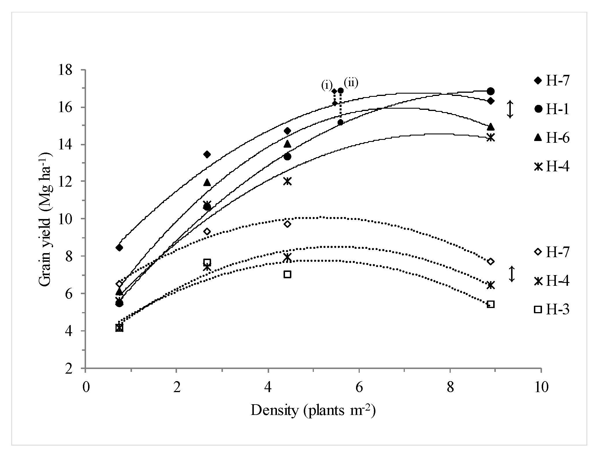
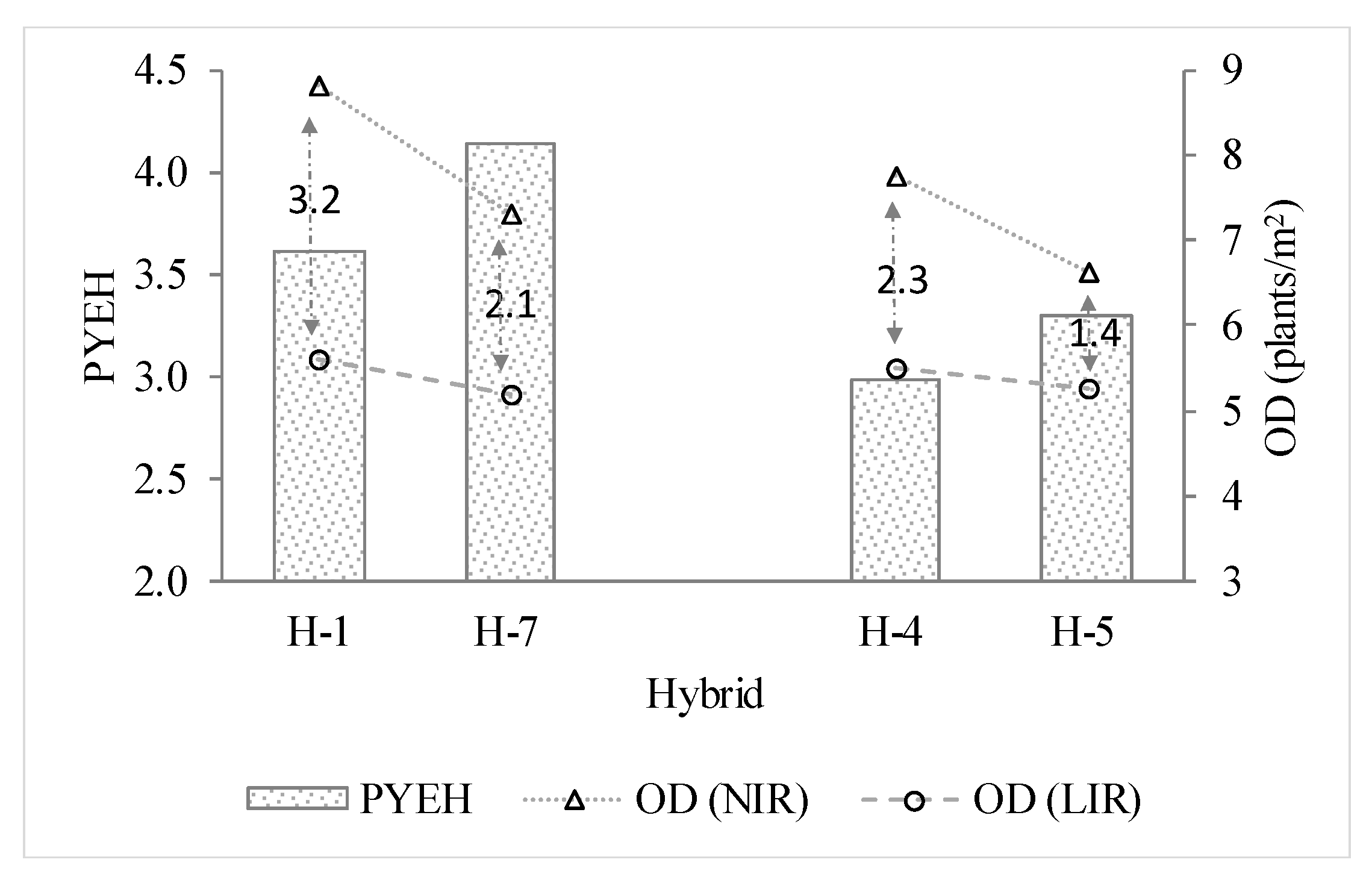
Hybrid	Quadratic Equation	OD	ACY 1	Quadratic Equation	OD	ACY
	NIR			LIR
H-1	Y = −0.17x2 + 3.03x + 3.48 (0.99)	8.81	16.82 a	Y = −0.21x2 + 2.34x + 3.21 (0.97)	5.61	9.77 a
H-2	Y = −0.21x2 + 2.95x + 3.23 (0.96)	7.00	13.56 d	Y = −0.19x2 + 2.00x + 2.68 (0.83)	5.27	7.94 c
H-3	Y = −0.20x2 + 2.76x + 3.72 (0.97)	7.05	13.46 d	Y = −0.17x2 + 1.75x + 3.31 (0.82)	5.11	7.78 c
H-4	Y = −0.17x2 + 2.72x + 3.99 (0.97)	7.77	14.54 c	Y = −0.18x2 + 2.01x + 2.97 (0.96)	5.51	8.51 b
H-5	Y = −0.27x2 + 3.57x + 2.55 (0.99)	6.64	14.38 c	Y = −0.21x2 + 2.26x + 2.33 (0.97)	5.26	8.28 bc
H-6	Y = −0.25x2 + 3.50x + 3.90 (0.98)	6.89	15.95 b	Y = −0.22x2 + 2.32x + 3.69 (0.98)	5.25	9.79 a
H-7	Y = −0.19x2 + 2.71x + 6.82 (0.97)	7.32	16.74 a	Y = −0.17x2 + 1.80x + 5.42 (0.97)	5.18	10.08 a
LSD			0.48			0.46

¹ Values followed by the same letter did not differ significantly at p < 0.05 on least significant difference (LSD) obtained from analysis of variance [20].

and partly illustrated in Figure 2. In the NIR, the OD ranged between 6.64 and 8.81 plants/m² (for H-5 and H-1, respectively), while in the LIR, all seven hybrids displayed narrow spread between 5.11 and 5.61 plants/ha. H-1 and H-7 showed the highest yield potential and equivalent ACY in both NIR (⸟16.8 Mg/ha) and LIR (⸟9.9 Mg/ha). These yield ceilings were attainable at quite similar ODs in the LIR (5.61 vs. 5.18 plants/m²), but differing by 1.49 plants/m² in the NIR (8.81 vs. 7.32 plants/m²). Similarly, at a significantly lower ACY, another pair of equivalent hybrids included H-4 and H-5 (⸟14.5 Mg/ha in the NIR and ⸟8.50 Mg/ha in the LIR), that exhibited comparable OD values in the LIR (5.51 vs. 5.26 plants/m²), but different in the NIR (7.77 vs. 6.64 plants/m²). The lowest yielding pair consisted of H-2 and H-3 that had similar optimum densities even in the NIR. The ACY of H-6 was proximate to that of the first pair in the LIR and slightly lower (by 5%) in the NIR.

The genotype ranking based on different stability estimating methods is presented in

Table 2. Hybrid ranking according to statistics appraising stability, i.e., GGE biplot, parametric ($AS{V}_i$, $P_i$ , b_i/=1, b_i/>1, ${\sigma }_i^2$, $\mathrm{a}C{V}_i$, $s_{xi}^2$, $s_{di}^2$ ) and non-parametric measures (S_i, NP_i, TMB, I_i), as well as the sum of ranking, at the low crop density (LCD), and the high crop density (HCD). At the bottom of each density-group, the range of absolute values is also given. On the right part it is shown the number of times each hybrid was 1st, 2nd, etc.

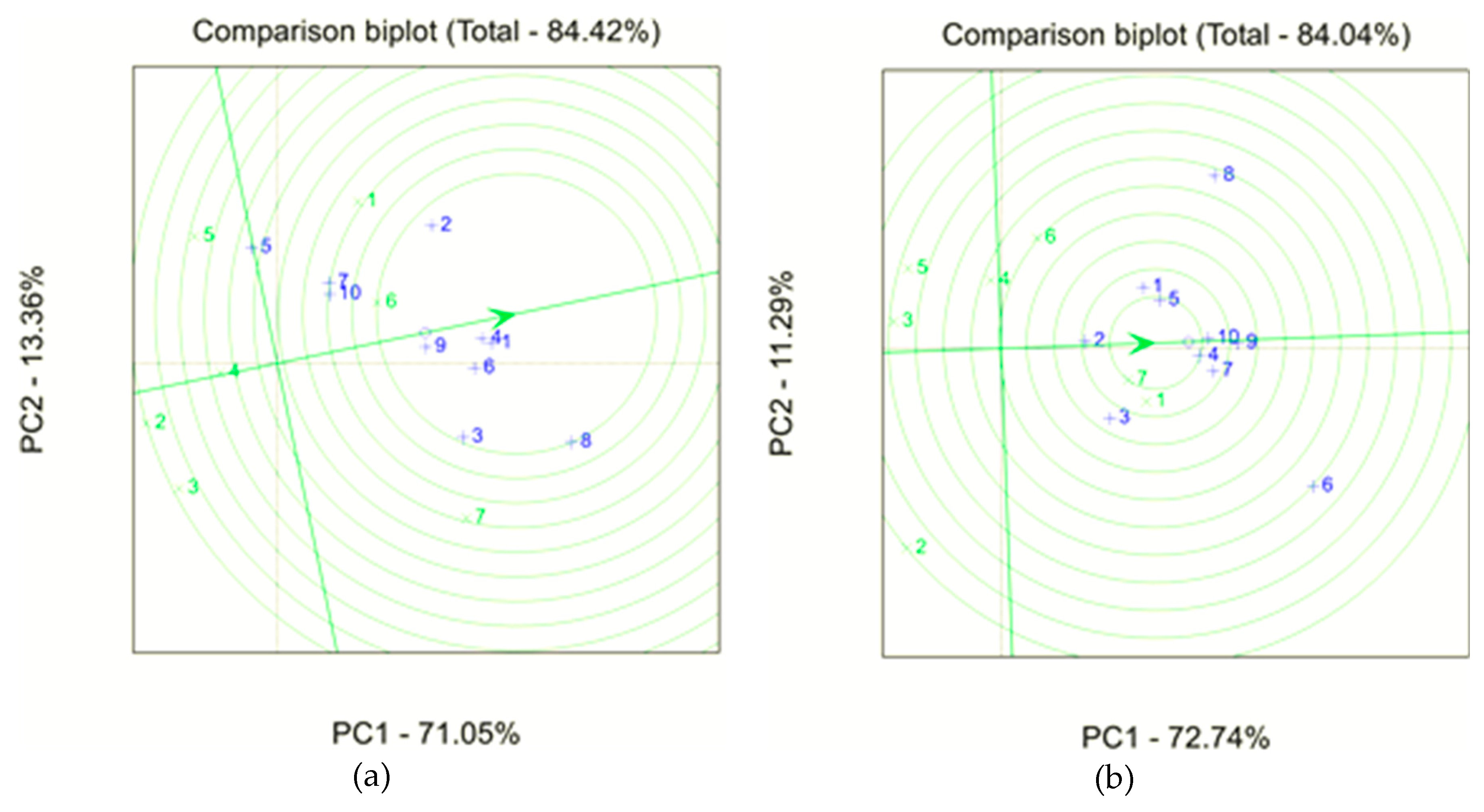
Hybrid	GGE	ASVi	Pi	bi/=1	bi/>1	${\mathit{\sigma }}_{\mathit{i}}^2$	aCVi	${\mathit{s}}_{\mathit{x}\mathit{i}}^2$	${\mathit{s}}_{\mathit{d}\mathit{i}}^2$	Si	NPi	TMB	Ii	SUM	1st	2nd	3rd	4th	5th	6th	7th
	LCD
H-1	2	5	3	7	7	5	1	5	5	5	5	3	3	56	1	1	3	0	6	0	2
H-2	7	4	7	2	5	4	6	6	4	2	3	6	7	63	0	2	1	3	1	3	3
H-3	6	1	6	1	4	1	5	2	1	1	1	7	6	42	6	1	0	1	1	3	1
H-4	4	2	4	4	6	2	3	1	2	3	2	5	5	43	1	4	2	3	2	1	0
H-5	5	6	5	5	2	6	7	4	6	6	4	4	4	64	0	1	0	4	3	4	1
H-6	1	3	2	3	3	3	2	3	3	4	6	1	2	36	2	3	6	1	0	1	0
H-7	3	7	1	6	1	7	4	7	7	7	7	2	1	60	3	1	1	1	0	1	6
Range		0.07–6.35	1.21–8.35	0.01–0.14	0.86–1.10	0.05–3.97	0.22–0.31	0.68–5.82	0.45–1.66	0.67–6.55	0.20–1.26	12–27	10–25
	HCD
H-1	2	7	2	7	1	6	4	7	2	7	6	2	3	56	1	4	1	1	0	2	4
H-2	7	6	6	6	7	7	5	5	7	2	1	6	6	71	1	1	0	0	2	5	4
H-3	6	2	7	4	6	5	6	4	4	3	3	5	7	62	0	1	2	3	2	3	2
H-4	4	5	4	2	4	3	3	1	5	4	5	4	4	48	1	1	2	6	3	0	0
H-5	5	3	5	3	5	2	7	3	3	1	2	7	5	51	1	2	4	0	4	0	2
H-6(	3	4	3	1	3	4	2	2	6	5	4	3	2	42	1	3	4	3	1	1	0
H-7	1	1	1	5	2	1	1	6	1	6	7	1	1	34	8	1	0	0	1	2	1
Range		0.81–1.47	0.14–6.78	0.01–0.17	0.89–1.17	0.58–1.46	0.39–0.45	0.86–4.18	0.39–1.10	1.45–4.74	0.33–1.19	14–28	5–25

; the sum of ranking is the overall score accepting the lowest as the best and the highest as the worst (for the GGE biplot analysis the scatter graphs are shown in Figure 3). The top hybrid for ACY, H-1, rarely ranked first (once at the LCD on $\mathrm{a}C{V}_i$ and once at the HCD on b_i/>1) and showed a relatively poor total ranking score. Its counterpart for ACY, H-7, showed the second-worst total score in the LCD, although it was first on P_i, b_i/>1 and I_i. Inversely in the HCD, H-7 showed the best overall score (34) and ranked first for eight out of the 13 stability criteria. The lowest hybrid for ACY, H-3, was prominent in the LCD, taking the lead in six out of the 13 stability standards and displaying the second better total score (42). Hybrids H-5 and H-2 had the worst total rankings; they gained the first position only once in the HCD and neither reach the top for any stability statistic in the LCD. H-6 achieved the best total score in the LCD and the second-best in the HCD, however, it gained the first position only twice in the LCD (GGE and TMB) and once in the HCD (b_i/=1).

3.3. Breeding Density Versus Dense Stand

Analyzing the top pair of hybrids for ACY, it is obvious that a higher PYEH value exhibited by H-7 compared to H-1 was followed by a reduced gap in the OD (2.1 vs. 3.2 plants/m²) as depicted in Figure 4. Similarly, H-5 had a higher PYEH and a lower gap in the OD than H-4 (1.4 vs. 2.3 plants/m²).

The overall yield at the BD, represented by PYE, was 21% lower in the LIR compared to the NIR; respectively, at the dense stand, the overall yield expressed by ACY, was 41% lower (Figure 5a). The greatest difference between genotypes for yield was 43% at the BD and ~21% at the dense stand, including both NIR and LIR (Figure 5b).

Simple correlations for grain yield among the ten sites by irrigation regimes for the seven genotypes are presented in

Table 3. Simple correlation coefficients among the ten environments (five sites at the normal irrigation regime, (NI), and the low irrigation regime, (LI), for grain yield of seven hybrids at the breeding density (BD), the low crop density (LCD), and the high crop density (HCD).

	Site2(NI)	Site3(NI)	Site4(NI)	Site5(NI)	Site1(LI)	Site2(LI)	Site3(LI)	Site4(LI)	Site5(LI)
	BD (0.74 plants/m2)
Site1(NI)	0.90 **	0.93 **	0.94 **	0.86 *	0.79 *	0.91 **	0.94 **	0.94 **	0.81 *
Site2(NI)	0.82 *	0.92 **	0.91 **	0.84 *	0.88 **	0.91 **	0.95 **	0.82 *
Site3(NI)	0.86 *	0.96 ***	0.78 *	0.97 ***	0.88 **	0.96 ***	0.85 *
Site4(NI)	0.89 **	0.87 *	0.92 **	0.90 **	0.76 *	0.92 **
Site5(NI)	0.91 **	0.96 ***	0.94 **	0.90 **	0.88 **
Site1(LI)	0.89 **	0.93 **	0.84 *	0.79 *
Site2(LI)	0.87 *	0.88 **	0.75
Site3(LI)	0.86 *	0.87 *
Site4(LI)	0.95 ***
	LCD (4.44 plants/m2)
Site1(NI)	0.33	0.16	−0.26	0.95 **	0.82 *	−0.01	0.63	0.59	0.95 **
Site2(NI)	−0.55	0.66	−0.35	0.90 **	0.32	−0.01	0.24	0.58
Site3(NI)	0.79 *	0.66	−0.57	0.23	0.48	0.75	0.47
Site4(NI)	0.79 *	0.41	0.39	0.28	0.88 **	0.79 *
Site5(NI)	0.82 *	0.04	0.20	0.85 *	0.93 **
Site1(LI)	0.13	0.46	−0.34	0.90 **
Site2(LI)	0.38	0.57	−0.28
Site3(LI)	0.95 **	0.53
Site4(LI)	0.89 **
	HCD (8.89 plants/m2)
Site1(NI)	0.13	0.49	0.90 **	0.68	0.69	0.56	0.68	0.76 *	0.88 **
Site2(NI)	0.74	0.65	0.68	0.81 *	0.80 *	0.74	0.73	0.92 **
Site3(NI)	0.61	0.26	0.74	0.61	0.77 *	0.45	0.86 *
Site4(NI)	0.73	0.25	0.81 *	0.87 *	0.81 *	0.78 *
Site5(NI)	0.38	0.22	0.91 **	0.72	0.89 **
Site1(LI)	0.75	0.46	0.72	0.87 *
Site2(LI)	0.78 *	0.72	0.92 **
Site3(LI)	0.62	0.51
Site4(LI)	0.73

Non-marked r values are not significant, while those marked are significant (*, p < 0.05; **, p < 0.01; *** p < 0.001).

. Because of the low degrees of freedom (df = 5) only large r values would be considered significant, i.e., above 0.75, 0.87, and 0.95 at p < 0.05, 0.01, and 0.001, respectively. Nevertheless, at the BD 44 out of the 45 simple correlations were significant, while the non-significant one was slightly lower than the reference value for p < 0.05. In contrary, a third of these correlations were significant at the LCD and HCD, respectively.

When the PYE was paired with ACY, the simple correlation was not significant in the NIR (r = 0.66) and significant in the LIR (r = 0.87, p < 0.05). The PYH ⸟ ACY correlations were very low in both NIR (r = 0.16) and LIR (r = 0.08). Nevertheless, the PYEH ⸟ ACY correlations were significant in both NIR (r = 0.84, P < 0.05) and LIR (r = 0.91, p < 0.01).

4. Discussion

In rainfed maize production, the strong hybrid by plant density by environment interaction is a crucial factor that prevents optimal productivity [22,25,32,40]. From this viewpoint, the results of this study were thoroughly discussed in a previous paper by Mylonas et al. [28]. Here, the main implications relevant to the scope of the present paper are summarized below.

All hybrids displayed a ⸟40% divergence in the ACY because of different irrigation and fertilization regimes (Table 1). Maize can be affected by climate change, and yield reductions between 10% and 30% have been reported depending on climate change scenario and type of hybrid used [41]. Concerning irrigated Mediterranean environments, divergence in grain yields was also reported for different pH and Zn levels [42], as well as various sowing dates [43]; yields under optimal pH-Zn levels and normal sowing dates were comparable to the high ACY levels computed for the NIR. Hybrids were also divergent in OD, which was lower in the LIR compared to NIR (on average 5.31 vs. 7.35 plants/m²). Interestingly, the difference in the OD gap was considerable in the NIR but only slight in the LIR (by 2.17 and 0.50 plants/m², respectively). Therefore, two crucial conclusions emerged. First, input-deficit conditions necessitate crop spacing irrespective of the hybrid. Second, hybrids demanding high densities to accomplish their yield potential under favorable conditions are prone to erratic OD; these are characterized as “density-dependent” hybrids and may harbor great risk of yield penalty across diverse growing conditions [22,25,32,40]. The remedy lies in the improvement of PYE aiming toward lowering the threshold of OD in favorable environments and bridging the gap in OD between stressful and favorable seasons, so as to develop “density-independent” hybrids that perform well with crop spacing even in seasons with adequate rainfalls. Indeed, analyzing the three hybrids that displayed the highest ACY, H-1 was specifically adapted to high densities and seasons with adequate rainfalls, H-6 was affected by high densities and specifically adapted to dry seasons, while H-7 was the most appropriate one for fluctuating environments due to the narrow OD gap.

Looking at stability through the prism of density dependence, it is apparent that for dryland maize production, the LCD in this study was close to the desired low crowding conditions in seasons with insufficient rainfall, while the HCD was more representative of optimum densities during seasons with adequate rainfalls. Consequently, a density close to the LCD would be preferred by a cautious farmer because of the fear of drought. In contrast, a bold farmer would establish a density proximate to the HCD hoping for the highest possible grain yields. For that reason, the stability statistics were computed at the HCD and LCD separately.

4.1. Genotype Ranking on Stability Measures

The statistics that better matched the ACY were GGE biplot, genotype superiority ($P_i$), stratified ranking procedure (TMB), and rank-sum index ($I_i$) (Table 2). Ranking on GGE in the HCD (Figure 3) was similar to that obtained when the two density regimes were analyzed together [28]. Several studies recommended the aforementioned stability criteria to promote the highest yielding genotypes and agronomic concept of stability [4,5,7,18,44,45]. Based on these, the highest yielding hybrids H-1, H-6, and H-7 were at the top of the list. Analyzing the two $b_i$ options, also assumed relevant to the agronomic concept of stability, only the more dynamic option, $b_{i/>1}$, was in accordance with ACY, and H-1 was graded the most undesirable on both $b_i$ options in the LCD. According to the remaining criteria, the low-yielding hybrids were prominent. A connection between the statistics of $AS{V}_i$, stability variance (${\sigma }_i^2$), coefficient of variation ($\mathrm{a}C{V}_i$), environmental variance ($s_{xi}^2$), variance of deviations from regression ($s_{di}^2$), $S_i$, and $N{P}_i$, associated them with the static concept of stability that allows the identification of genotypes adapted to environments with unfavorable growing conditions [3,4,5,7,16,46]. Nevertheless, such a connection is not evidenced in this study. Notably, in the LCD that represents a relatively optimal density for input-deficit environments, H-3 was rated excellent by these criteria, although it lagged behind the rest of the hybrids in both yield and stability even in the LIR (Table 1, Figure 2). In general, genotype ranking based on $b_i$ and $\mathrm{a}C{V}_i$ is reproducible, while reproducibility of ${\sigma }_i^2$, $S_{xi}^2$, and $S_{di}^2$ is low [1,12,47,48]. Mendes and Ramalho [48] also found mean of the absolute scores weighed through the explanation of each PC of AMMI to have low repeatability. The statistics of $S_i$, $N{P}_i$, and $\mathrm{a}C{V}_i$ are influenced by yield and stability simultaneously, so that genotypes selected based on them show average stability and may not be as efficient as genotypes responsive under favorable conditions [7]. The static aspect of stability compromises methods that favor genotypes with moderate yield and high stability [4]; this is not acceptable by most agronomists and breeders who prefer genotypes with high mean yields that respond to agronomic inputs or favorable environmental conditions [12].

Τhe above criteria were conflicting, thus inadequate to single out any hybrid for both yield and stability. In many studies, hybrids have been shown to respond dramatically differently to diverse density conditions [37,49], which was also the case here. In the LCD, the high-yield potential hybrid, H-7, ranked first three times compared to the low yield potential hybrid, H-3, that ranked first in most of the criteria (6), thus receiving a good total score in contrast to H-7 (Table 2). H-7 was also underestimated based on the total score in comparison with the low-yielding H-4. Interestingly, the specifically adapted to low-input environments H-6, although scoring the best total in the LCD, would only be selected based on GGE or TMB. In the HCD, the tolerant to high densities H-1 was underestimated compared to the susceptible to crowding H-6 and the low-yielding H-4. These inferences are further discussed below in combination with the statistics applied at the BD.

4.2. The Prediction Value of the PYEH for Yield and Stability Across Densities

In general, hybrids that exhibited high PYEH values performed analogously in terms of ACY. The hybrid grouping according to PYEH in Figure 1 coincided perfectly with their pairing based on ACY. Interesting inferences were drawn when a comparison was made within each of the top and intermediate ACY hybrid pairs.

Under the optimal NIR conditions, H-1 showed a more drastic yield decline with decreasing density compared to H-7 (Figure 2) because of the inability of the former to use inputs at low densities, i.e., low PYE (Figure 1). The demand for high densities when there are adequate inputs is the consequence of low PYE, which constitutes a root cause of unstable OD and high potential yield loss across fluctuating seasons [22,25]. In a hypothetical scenario, if a cautious farmer prefers the low optimum densities recommended for LIR due to fear of drought, then according to Figure 2 in a season with rainfalls sufficient to simulate the NIR the yield loss for H-1 would be 1.76 Mg/ha (11%) compared to 0.84 Mg/ha (5%) for H-7. On the other extreme (not shown), if a venturous farmer opts for the high optimum densities suggested for the NIR aiming toward the greatest possible grain yields, then in a season similar to the LIR the yield loss for H-1 would be 2.13 Mg/ha (22%), while the respective yield loss for H-7 would be 0.79 Mg/ha (8%). In any case, it is obvious that environmental fluctuation would have a more drastic effect on H-1 performance, so that cultivation of H-7 with crop spacing seemed comparatively a viable option. Because of the improved PYE, H-7 exhibited greater stability and better adaptation to lower densities [28], which is a prerequisite for stability in dryland maize production [22,25,34]. Such a hybrid could be planted at the prone for a dry season low density without compromising the attainable grain yield during seasons with adequate rainfall due to the ability of individual plants to utilize additional inputs.

The level of adaptation to crop spacing is also highlighted by comparing H-7 to H-1 or H-5 to H-4 in terms of OD spread in NIR versus LIR (Figure 4). It seems that stability in fluctuating conditions is associated with improved PYEH. It is worth mentioning that, while improved PYEH was the result of improved PYE rather than PYH for H-7, the opposite was true for H-5. It stands to reason that improved PYE is a determining factor in lowering the threshold of OD under optimal conditions [25,28,31]. The contribution of improved PYH (i.e., low plant-to-plant variability) to stability may be related to the level of intra-crop variation. Given the genetic homogeneity of hybrids, plant-to-plant variation is caused entirely by the environment, i.e., acquired heterogeneity and interplant inequality [34]. Hence, high PYH may reflect the ability of a genotype to withstand exogenous forces that enhance interplant differences. Most likely the performance of H-7 would be even more stable if PYH was also improved.

The analyses based on PYEH and ACY coincided perfectly compared to GGE biplot, $P_i$, TMB, and $I_i$, which are also tools used to highlight high-yielding genotypes. Although a crop of different growth habit and yield formation, in a dry bean (Phaseolus vulgaris L.) study, PYEH was in alignment with these four stability measures in identifying the outstanding among 21 genotypes [44]. In this study, PYEH was also indispensable in order to pinpoint genotypes expected to yield optimally at a wide range of densities and thus alleviate the problem of erratic OD [22,28]. In that case, PYEH could be a powerful tool to quickly evaluate whether existing hybrids meet the requirements emanating from environmental vulnerability.

4.3. Implications of Breeding at the BD

The improvement of single-plant performance is imperative to develop crops adapted to accomplish optimal yield at low densities inter-seasonally, which constitutes a strategy toward resilience during less favorable seasons. The results of this study demonstrated that PYEH could be a powerful selection tool in breeding programs at ultra-low densities (BD) that neutralize plant-to-plant interference for inputs.

Water stress affected yield more drastically at the dense stand than at the BD (Figure 5a) in accordance with the general consensus that drought effects are more pronounced at high densities [28,32,40]. Thus, BD facilitates a much better (theoretically maximum) phenotypic expression even under stress conditions that could intensify the differences among genotypes. Indeed, the magnitude of genotype differentiation was greater at the BD (Figure 5b). This comes as the result of the fact that yielding capacity of individual plants approaches full expression at the BD; consequently, maximum phenotypic expression leads to maximum phenotypic differentiation [33,34].

In terms of yield, hybrids were consistent at the BD (PYE) but at the dense stand (ACY) across diverse environmental conditions determined by site and input level. Even though a risky assumption and further small degrees of freedom make it necessary to consider the r values of Table 3 with caution, this finding corroborated our previous study, including 30 parent lines and 31 hybrids [27]. Comparing BD with LCD and HCD, the impact of the GE interaction seems to differ. The significant correlations found when plants were widely spaced indicates that the GE interaction at the BD may vary in scale because of the temporal and spatial variation but does not alter the genotype ranking. This means that, although such non-crossover quantitative type of GE is unavoidable in field experiments [50], it would not prevent the identification of superior genotypes. In contrast, a reduced association between phenotypic and genotypic values under crowding in dense stands (LCD and HCD), leads to variations in genotype classification from one environment to another (the qualitative or crossover GE aspect), thus impeding the recognition of superior genotypes [51,52].

By eliminating interplant competition, BD conditions seem to promote heritability more efficiently than dense stand. Indicatively, there were recorded smaller effects of input shortage in the LIR, greater phenotypic expression and differentiation for PYE compared to ACY in both NIR and LIR, and consistency in hybrid ranking across environments. The impact of GE interaction increases while genetic variance and heritability decline when crowding and environmental stress intensify [53,54]. Heritability is further boosted by the fact that BD alleviates the effects of the negative relationship between competitive and yielding ability [33,34].

The reasonable question of whether PYEH and its components are transferable to farming conditions could be partly answered by examining closer the development of H-7, in which case both parent lines resulted by breeding at the BD based more on PYE and much less on PYH [27]. In this study, although there was a positive correlation between ACY and PYEH, ACY only partly related to PYE, while no such relationship was apparent with PYH. Nevertheless, there is mounting evidence in various crops that the performance of widely spaced plants reflects yield under densely seeded situations (e.g., [44,55,56,57,58]). In maize inbred lines and hybrids, the performance across six environments at farming dense stand exhibited a better correlation with individual trials conducted at nil-competition compared with those at dense stand [27]. Hansen et al. [59] also speculated that selection in space-planted nurseries in one trial for subsequent performance in multiple environments is a realistic scenario. Still the establishment of PYH as a practical stability index merits further investigation. Interplant inequality intensifies the intraspecific competition and is related to reduced grain yield productivity [60,61,62]. Thus, addressing intraspecific competition may be beneficial for breeding high-yielding varieties [63,64]. Presumably, high PYH values are indicative of a genetic background that promotes resilience to acquired interplant variation. Since improved PYE is related with the “weak competitor” ideotype, combined with increased PYH would moderate the acquired intra-crop variation and mitigate the intraspecific competition, thus promoting yield and stability at the same time.

In conclusion, maize cropping system requires versatile hybrids that exhibit plasticity to environmental diversity [24]. A lower yield penalty in low-density management strategies would characterize a crop stable in drought-prone areas that is adapted to tolerate drought stress [65]. The development of density-independent hybrids based on improved PYEH would serve this purpose, i.e., independence of crop yield from seeding rate, mitigation of intra-crop variation, better compensation for missing plants and ability to fully exploit drought-prone environments [34].

5. Conclusions

The scope of the study was to analyze hybrid stability in terms of density-dependence focusing on the potential yield loss due to erratic optimum density in rainfed maize crops. Most of the parametric and non-parametric stability measures based on yield performance at crop densities gave conflicting results regarding hybrids that stood out for both yield and stability except for GGE biplot, P_i, TMB, and I_i. This inconsistency was more pronounced at the optimal for dryland production LCD. In contrast, when PYEH, a statistic tool based on single-plant yield performance at an ultra-low density, was employed for prognostic purposes, high-yielding and stable genotypes were highlighted, which moreover had the potential to reach the season’s attainable crop yield with crop spacing. High PYEH values entail increased single-plant yield and reduced interplant variation, thus are indicative of individual plants efficient in resource use, which lead to crops adapted to low densities via bridging the inter-seasonal gap in optimum density and able to reach optimal crop yield irrespective of crop spacing even in favorable seasons. Crop spacing is an inviolable rule under resource-deficit conditions, so crop adaptation to low densities is a viable option to alleviate the major problem of erratic optimum density. The results were further supportive of breeding at ultra-low density rather than crop densities to facilitate the identification and selection of superior genotypes, since such conditions promote phenotypic expression and differentiation, and ensure repeatability across diverse environments. Undoubtedly, breeding based on PYEH could lead to density-independent hybrids that exhibit resilience to environmental vulnerability through crop yield independence from seeding rate, mitigation of intra-crop variation, better compensation for missing plants, and ability to exploit drought-prone environments.

References

- Baxevanos, D.; Goulas, C.; Tzortzios, S.; Mavromatis, A. Interrelationship among and repeatability of seven stability indices estimated from commercial cotton (Gossypium hirsutum L.) variety evaluation trials in three Mediterranean countries. Euphytica 2008, 161, 371–382. [Google Scholar] [CrossRef]
- Basu, S.K.; Acharya, S.N.; Bandara, M.S.; Friebel, D.; Thomas, J.E. Effects of genotype and environment on seed and forage yield in fenugreek (Trigonella foenum-graecum L.) grown in western Canada. Aust. J. Crop Sci. 2009, 3, 305–314. [Google Scholar]
- Akcura, M.; Kaya, Y.; Taner, S.; Ayranci, R. Parametric stability analyses for grain yield of durum wheat. Plant Soil Environ. 2006, 52, 254–261. [Google Scholar] [CrossRef] [Green Version]
- Sabaghnia, N.; Dehghani, H.; Sabaghpour, S.H. Nonparametric methods for interpreting genotype x environment interaction of lentil genotypes. Crop Sci. 2006, 46, 1100–1106. [Google Scholar] [CrossRef]
- Solomon, K.F.; Smit, H.A.; Malan, E.; Du Toit, W.J. Comparison study using rank based nonparametric stability statistics of durum wheat. World J. Agric. Sci. 2007, 3, 444–450. [Google Scholar]
- Fikere, M.; Tadesse, T.; Gebeyehu, S.; Hundie, B. Agronomic performances, disease reaction and yield stability of field pea (Pisum sativum L.) genotypes in Bale Highlands, Ethiopia. Aust. J. Crop Sci. 2010, 4, 238–246. [Google Scholar]
- Mohammadi, R.; Amri, A. Comparison of parametric and non-parametric methods for selecting stable and adapted durum wheat genotypes in variable environments. Euphytica 2008, 159, 419–432. [Google Scholar] [CrossRef]
- Hühn, M.; Leon, J. Non-parametric analysis of cultivar performance trials: Experimental results and comparison of different procedures based on ranks. Agron. J. 1995, 87, 627–632. [Google Scholar] [CrossRef]
- Finlay, K.W.; Wilkinson, G.N. The analysis of adaptation in a plant breeding programme. Aust. J. Agric. Res. 1963, 14, 742–754. [Google Scholar] [CrossRef] [Green Version]
- Eberhart, S.A.; Russell, W.A. Stability parameters for comparing varieties. Crop Sci. 1966, 6, 36–40. [Google Scholar] [CrossRef] [Green Version]
- Lin, C.S.; Binns, M.R.; Lefkovitch, L.P. Stability analysis: Where do we stand? Crop Sci. 1986, 26, 894–900. [Google Scholar] [CrossRef] [Green Version]
- Becker, H.C.; Leon, J. Stability analysis in plant breeding. Plant Breed 1988, 101, 1–23. [Google Scholar] [CrossRef]
- Shukla, G.K. Some statistical aspects of partitioning genotype–environmental components of variability. Heredity 1972, 29, 237–245. [Google Scholar] [CrossRef] [PubMed]
- Francis, T.R.; Kannenberg, L.W. Yield stability studied in short-season maize: I. A descriptive method for grouping genotypes. Can. J. Plant Sci. 1978, 58, 1029–1034. [Google Scholar] [CrossRef]
- Lin, C.S.; Binns, M.R. A method of analyzing cultivar x location x year experiments: A new stability parameter. Theor. Appl. Genet. 1988, 76, 425–430. [Google Scholar] [CrossRef] [PubMed]
- Nassar, R.; Huehn, M. Studies on estimation of phenotypic stability: Tests of significance for nonparametric measures of phenotypic stability. Biometrics 1987, 43, 45–53. [Google Scholar] [CrossRef]
- Fox, P.N.; Skovmand, B.; Thompson, B.K.; Braun, H.J.; Cormier, R. Yield and adaptation of hexaploid spring triticale. Euphytica 1990, 47, 57–64. [Google Scholar] [CrossRef]
- Kang, M.S.; Pham, H.N. Simultaneous selection for high yielding and stable crop genotypes. Agron. J. 1991, 83, 161–165. [Google Scholar] [CrossRef]
- Gauch, H.G. Statistical analysis of yield trials by AMMI and GGE. Crop Sci. 2006, 46, 1488–1500. [Google Scholar] [CrossRef]
- Yan, W. Singular-value partition in biplot analysis of multienvironment trial data. Agron. J. 2002, 94, 990–996. [Google Scholar] [CrossRef] [Green Version]
- Purchase, J.L.; Hatting, H.; Van Deventer, C.S. Genotype × environment interaction of winter wheat in South Africa: II. Stability analysis of yield performance. S. Afr. J. Plant Soil 2000, 17, 101–107. [Google Scholar] [CrossRef]
- Tokatlidis, I.S. Adapting maize crop to climate change. Agron. Sustain. Dev. 2013, 33, 63–79. [Google Scholar] [CrossRef] [Green Version]
- Xu, W.; Liu, C.; Wang, K.; Ruizhi, X.; Ming, B.; Wang, Y.; Zhang, G.; Liu, G.; Zhao, R.; Fan, P.; et al. Adjusting maize plant density to different climatic conditions across a large longitudinal distance in China. Field Crops Res. 2017, 212, 126–134. [Google Scholar] [CrossRef]
- Seyoum, S.; Rachaputi, R.; Fekybelu, S.; Chauhana, Y.; Prasanna, B. Exploiting genotype x environment x management interactions to enhance maize productivity in Ethiopia. Eur. J. Agron. 2019, 103, 165–174. [Google Scholar] [CrossRef]
- Duvick, D.N. The contribution of breeding to yield advances in maize (Zea mays L.). Adv. Agron. 2005, 86, 83–145. [Google Scholar]
- Brekke, B.; Edwards, J.; Knapp, A. Selection and adaptation to high plant density in the Iowa stiff stalk synthetic maize (Zea mays L.) population. Crop Sci. 2011, 51, 1965–1972. [Google Scholar] [CrossRef]
- Tokatlidis, I.S.; Dordas, C.; Papathanasiou, F.; Papadopoulos, I.; Pankou, C.; Gekas, F.; Ninou, E.; Mylonas, I.; Tzantarmas, C.; Petrevska, J.K.; et al. Improved plant yield efficiency is essential for maize rainfed production. Agron. J. 2015, 107, 1011–1018. [Google Scholar] [CrossRef] [Green Version]
- Mylonas, I.; Sinapidou, E.; Remountakis, E.; Sistanis, I.; Pankou, C.; Ninou, E.; Papadopoulos, I.; Papathanasiou, F.; Lithourgidis, A.; Gekas, F.; et al. Improved plant yield efficiency alleviates the erratic optimum density in maize. Agron. J. 2020, 112, 1690–1701. [Google Scholar] [CrossRef]
- Ciampitti, I.A.; Vyn, T.J. Understanding global and historical nutrient use efficiencies for closing maize yield gaps. Agron. J. 2014, 106, 2107–2117. [Google Scholar] [CrossRef] [Green Version]
- Gonzalez, V.H.; Tollenaar, M.; Bowman, A.; Good, B.; Lee, E.A. Maize yield potential and density tolerance. Crop Sci. 2018, 58, 472–485. [Google Scholar] [CrossRef]
- Assefa, Y.; Carter, P.; Hinds, M.; Bhalla, G.; Schon, R.; Jeschke, M.; Paszkiewicz, S.; Smith, S.; Ciampitti, I.A. Analysis of long term study indicates both agronomic optimal plant density and increase maize yield per plant contributed to yield gain. Sci. Rep. 2018, 8, 4937. [Google Scholar] [CrossRef] [PubMed] [Green Version]
- Berzsenyi, Z.; Tokatlidis, I.S. Density-dependence rather maturity determines hybrid selection in dryland maize production. Agron. J. 2012, 104, 331–336. [Google Scholar] [CrossRef]
- Fasoula, V.A.; Tokatlidis, I.S. Development of crop cultivars by honeycomb breeding. Agron. Sustain. Dev. 2012, 32, 161–180. [Google Scholar] [CrossRef] [Green Version]
- Tokatlidis, I.S. Crop adaptation to density to optimise grain yield: Breeding implications. Euphytica 2017, 213, 92. [Google Scholar] [CrossRef]
- Fasoulas, A.C.; Fasoula, V.A. Honeycomb selection designs. Plant Breed Rev. 1995, 13, 87–139. [Google Scholar]
- Qian, C.; Yu, Y.; Gong, X.; Jiang, Y.; Zhao, Y.; Yang, Z.; Hao, Y.; Li, L.; Song, Z.; Zhang, W. Response of grain yield to plant density and nitrogen rate in spring maize hybrids released from 1970 to 2010 in Northeast China. Crop J. 2013, 4, 459–467. [Google Scholar] [CrossRef] [Green Version]
- Amelong, A.; Hernández, F.; Novoa, A.D.; Borrás, L. Maize stand density yield response of parental inbred lines and derived hybrids. Crop Sci. 2017, 57, 32–39. [Google Scholar] [CrossRef]
- Thennarasu, K. On Certain Non-Parametric Procedures for Studying Genotype-Environment Interactions and Yield Stability. Ph.D. Thesis, P.J. School, IARI, New Delhi, India, 1995. [Google Scholar]
- Payne, R.W. Genstat. Wiley Interdis. Rev. Comp. Stat. 2009, 1, 255–258. [Google Scholar] [CrossRef]
- Solomon, K.F.; Chauhan, Y.; Zeppa, A. Risks of yield loss due to variation in optimum density for different maize genotypes under variable environmental conditions. J. Agron. Crop Sci. 2017, 203, 519–527. [Google Scholar] [CrossRef]
- Meza, F.J.; Silva, D.; Vigil, H. Climate change impacts on irrigated maize in Mediterranean climates: Evaluation of double cropping as an emerging adaptation alternative. Agr. Syst. 2008, 98, 21–30. [Google Scholar] [CrossRef]
- Nájera, F.; Tapia, Y.; Baginsky, C.; Figueroa, V.; Cabeza, R.; Salazar, O. Evaluation of soil fertility and fertilisation practices for irrigated maize (Zea mays L.) under Mediterranean conditions in central Chile. J. Soil Sci. Plant Nut. 2015, 15, 84–97. [Google Scholar] [CrossRef] [Green Version]
- Maresma, A.; Ballesta, A.; Santiveri, F.; Lloveras, J. Sowing date affects maize development and yield in irrigated Mediterranean environments. Agriculture 2019, 9, 67. [Google Scholar] [CrossRef] [Green Version]
- Papadopoulos, I.I.; Tokatlidis, I.S. A novel statistic estimated in the absence of competition to foresee genotype performance at the farming conditions parallels the agronomic concept of stability. Austr. J. Crop Sci. 2011, 5, 822–830. [Google Scholar]
- Kebede, A.; Getahun, A. Adaptability and Stability Analysis of Groundnut Genotypes Using AMMI Model and GGE-biplot. J. Crop Sci. Biotech. 2017, 20, 343–349. [Google Scholar] [CrossRef]
- Mekbib, F. Yield stability in common bean (Phaseoulus vulgaris L.) genotypes. Euphytica 2003, 130, 147–153. [Google Scholar] [CrossRef]
- Jalaluddin, M.D.; Harrison, S.A. Repeatability of stability statistics for grain yield in wheat. Crop Sci. 1993, 33, 720–725. [Google Scholar] [CrossRef]
- Mendes, M.H.S.; Ramalho, M.A.P. Repeatability of some phenotypic stability parameters - a resampling approach. Crop Breed Appl. Biot. 2018, 18, 139–147. [Google Scholar] [CrossRef] [Green Version]
- Dhaliwal, D.S.; Williams, M.M. Understanding variability in optimum plant density and recommendation domains for crowding stress tolerant processing sweet corn. PLoS ONE 2020, 15. [Google Scholar] [CrossRef] [Green Version]
- Sabaghnia, N.; Dehghani, H.; Alizadeh, B.; Mohghaddam, M. Diallele analysis of oil content and some agronomic traits in rapeseed (Brassica napus L.) based on the additive-dominance genetic model. Aust. J. Crop Sci. 2010, 4, 609–616. [Google Scholar]
- Romagosa, I.; Fox, P.N. Genotype × environment interaction and adaptation. In Plant breeding: Principles and Prospects; Hayward, M.D., Bosemark, N.O., Romagosa, I., Eds.; Chapman and Hall: London, UK, 1993; pp. 373–390. [Google Scholar]
- Baker, R.J. Tests for crossover genotype–environment interactions. Can J. Plant Sci. 1988, 68, 405–410. [Google Scholar] [CrossRef]
- Rosielle, A.A.; Hamblin, J. Theoretical aspects of selection for yield in stress and non-stress environments. Crop Sci. 1981, 21, 943–946. [Google Scholar] [CrossRef]
- Mansfield, B.D.; Mumm, R.H. Survey of plant density tolerance in U.S. maize germplasm. Crop Sci. 2014, 54, 157–173. [Google Scholar] [CrossRef] [Green Version]
- Ntanos, D.A.; Roupakias, D.G. Comparative efficiency of two breeding methods for yield and quality in rice. Crop Sci. 2001, 41, 345–350. [Google Scholar] [CrossRef]
- Tokatlidis, I.S.; Xynias, I.N.; Tsialtas, J.T.; Papadopoulos, I.I. Single-plant selection at ultra-low density to improve stability of a bread wheat cultivar. Crop Sci. 2006, 46, 90–97. [Google Scholar] [CrossRef]
- Fasoula, V.A.; Boerma, H.R. Intra-cultivar variation for seed weight and agronomic traits. Crop Sci. 2007, 47, 367–373. [Google Scholar] [CrossRef]
- Vlachostergios, D.N.; Lithourgidis, A.S.; Roupakias, D.G. Effectiveness of single plant selection at low density under organic environment. A field study with lentil. Crop Sci. 2011, 51, 41–51. [Google Scholar] [CrossRef]
- Hansen, K.A.; Martin, J.M.; Lanning, S.P.; Talbert, L.E. Correlation of genotype performance for agronomic and physiological traits in space-planted versus densely seeded conditions. Crop Sci. 2005, 45, 1023–1028. [Google Scholar] [CrossRef]
- Liu, W.; Tollenaar, M. Response of yield heterosis to increasing plant density in maize. Crop Sci. 2009, 49, 1807–1816. [Google Scholar] [CrossRef]
- Martin, K.L.; Hodgen, P.J.; Freeman, K.W.; Melchiori, R.; Arnall, D.B.; Teal, R.K.; Mullen, R.W.; Desta, K.; Phillips, S.B.; Solie, J.B.; et al. Plant-to-plant variability in corn production. Agron. J. 2005, 97, 1603–1611. [Google Scholar] [CrossRef] [Green Version]
- Tokatlidis, I.S.; Remountakis, E. The Impacts of interplant variation on aboveground biomass, grain yield, and harvest index in maize. Inter. J. Plant Prod. 2020, 14, 57–65. [Google Scholar] [CrossRef]
- Zhai, L.; Xie, R.; Ming, B.; Li, S.; Ma, D. Evaluation and analysis of intraspecific competition in maize: A case study on plant density experiment. J. Integr. Agric. 2018, 17, 2235–2244. [Google Scholar] [CrossRef] [Green Version]
- Shao, H.; Shi, D.; Shi, W.; Ban, X.; Chen, Y.; Ren, W.; Chen, F.; Mi, G. Genotypic difference in the plasticity of root system architecture of field-grown maize in response to plant density. Plant and Soil 2019, 439, 201–217. [Google Scholar] [CrossRef]
- Ross, F.; Di Matteo, J.; Cerrudo, A. Maize prolificacy: A source of reproductive plasticity that contributes to yield stability when plant population varies in drought-prone environments. Field Crops Res. 2020, 247, 107699. [Google Scholar] [CrossRef]