
Grain Yield Estimation in Rice Breeding Using Phenological Data and Vegetation Indices Derived from UAV Images


1
The State Key Laboratory of Soil and Sustainable Agriculture, Institute of Soil Science Chinese Academy of Sciences, Nanjing 210008, China
2
College of Advanced Agricultural Sciences, University of Chinese Academy of Sciences, Beijing 100049, China
*
Author to whom correspondence should be addressed.
Agronomy 2021, 11(12), 2439; https://0-doi-org.brum.beds.ac.uk/10.3390/agronomy11122439
Submission received: 19 October 2021
/
Revised: 28 November 2021
/
Accepted: 28 November 2021
/
Published: 29 November 2021
Abstract
:The accurate estimation of grain yield in rice breeding is crucial for breeders to screen and select qualified cultivars. In this study, a low-cost unmanned aerial vehicle (UAV) platform mounted with an RGB camera was carried out to capture high-spatial resolution images of rice canopy in rice breeding. The random forest (RF) regression techniques were used to establish yield models by using (1) only color vegetation indices (VIs), (2) only phenological data, and (3) fusion of VIs and phenological data as inputs, respectively. Then, the performances of RF models were compared with the manual observation and CERES-Rice model. The results indicated that the RF model using VIs only performed poorly for estimating yield; the optimized RF model that combined the use of phenological data and color VIs performed much better, which demonstrated that the phenological data significantly improved the model performance. Furthermore, the yield estimation accuracy of 21 rice cultivars that were continuously planted over three years in the optimal RF model had no significant difference (p > 0.05) with that of the CERES-Rice model. These findings demonstrate that the RF model, by combining phenological data and color Vis, is a potential and cost-effective way to estimate yield in rice breeding.
1. Introduction
Rice (Oryza sativa L.), one of the most important food crops in the world, is consumed by more than half of the global population [1], especially in East Asia and Southeast Asia. Food price fluctuations in the market can adversely affect rice cost and production; hence, a convenient and reliable technology for predicting rice yield is necessary for farmers and governments to make appropriate decisions in regard to rice production [2].
Traditionally, agronomists rely on field survey to obtain approximate yield predictions. However, estimation based on empirical and subjective knowledge resulted in inaccurate crop assessment and were limited in capacity for yield estimation in regional scale [3,4]. Satellite imagery-based remote sensing (RS) data have been widely used for monitoring crop growth status and nutritional conditions [5,6]. Yield prediction models were established based on meteorological factors and an RS vegetation index (VI) using the multiple linear regression technique [7], and it was found that the inclusion of remote sensing data could significantly improve the yield prediction accuracy. The enhanced vegetation index (EVI) and normalized difference vegetation index (NDVI) data derived from the moderate resolution imaging spectroradiometer (MODIS) were compared for estimating rice yield, and the result indicated that the EVI-based models were slightly more accurate than the NDVI-based models [1]. However, typically, satellite imagery had conflict between spatial and temporal resolutions, and the quality of RS data was considerably affected by atmospheric interference [8,9]. Although synthetic aperture radar (SAR) techniques that could penetrate vegetation canopies were not influenced by clouds [10,11], it was difficult to exactly extract crop information due to the small size of farmlands in the south of China. For understanding the effect of site-specific crop management and environmental stress on crop production, a highly accurate and reliable model for crop yield estimation in the plot-scale was essential [12].
As for plot-scale yield estimation, crop growth models have been successfully proposed to simulate yield such as DSSAT [13], AquaCrop [14], EPIC [15], and APSIM [16]. These models become efficient and useful tools for field management and precision agriculture [17]. The CERES-Rice model involved in the DSSAT model has been widely used as a technological tool to support the decision-making for rice field management activities [18,19]. The capability of the CERES-Rice model for rice yield estimation has been reported in previous studies [20,21,22]. However, the implementation of crop growth models (e.g., CERES-Rice) in commercial application remains limited because of their high data acquisition costs. For example, the soil properties need to be measured in the laboratory and the cultivar parameters need to be tuned costly. Moreover, the proper use of these models requires skillful manipulators with agronomic knowledge to obtain satisfactory results.
In recent years, unmanned aerial vehicle (UAV) with a high spatial resolution of imagery has attracted considerable interest for crop yield estimation in plot scale [23,24,25]. Feng et al. [26] extracted eight image features from a UAV system and found that the fusion of two image features could improve the accuracy of cotton yield estimation. Yang et al. [27] constructed the convolutional neural network (CNN) model with the dataset of RGB and multispectral images derived from UAV to estimate rice yield, and they found that the CNN’s accuracy in RGB image dataset was better than that in the multispectral image dataset. The VIs and crop height data extracted from UAV-RGB images with crop surface models (CSMs) were combined to estimate corn yield by three linear models [28]. Agueera Vega et al. [29] calculated NDVI from multi-temporal images obtained from a UAS and found that NDVI was highly correlated with grain yield. Furthermore, a good correlation also exists between the sugarcane yield and G–R vegetation index obtained by the UAV-RGB images [30].
Although most scholars have proven the potential of image features for crop yield estimation under the same crop cultivar, the yield estimation in breeding programs was still challenged by the variation of genotypes. In breeding trials, thousands of genotypes from two parents were planted without duplication. The great variation of phenotypes in yield could be caused by the combination of environmental and genetic variations [31]. Accordingly, only a few studies have been reported for yield estimation in crop breeding [32]. For example, Zhou et al. [32] used CNN to estimate the yield of 972 soybean breeding lines with R2 of 0.78 and RMSE of 391 kg ha−1 based on the UAV imagery. Ashapure et al. [33] demonstrated that a simple Artificial Neural Network (ANN) model could perform well for yield estimation in a set of tomato varieties by using UAV-RGB imagery.
To the best of the authors’ knowledge, previous studies focused on estimating the plot-scale crop yield by using image features from UAV-based imagery, and they neglected the growth duration that determined the amount of incident solar radiation closely associated with biomass and grain yield as an important phenological factor [34]. In rice breeding, the growth duration varied across cultivars; thus, the estimation of grain yield in rice breeding, only based on VIs from UAV images, could result in considerable uncertainty. The random forest (RF) regression technique has been successfully used to estimate crop biomass [35], grain yield [36], and nitrogen status [37]. Thus, in this study, RF was used to construct the yield estimation models. Meanwhile, the yield estimation of the same cultivars that were continuously planted over three years in the RF model was compared to the CERES-Rice model. Accordingly, the objectives of this study are: (1) to establish the RF model for yield estimation in rice breeding using UAV-based RGB images only; (2) to improve the capability of the RF model combining RGB images and phenological data; (3) to validate the performance of the optimal RF model, comparing it with that of the CERES-Rice model.
2. Materials and Methods
2.1. Field Trial Design
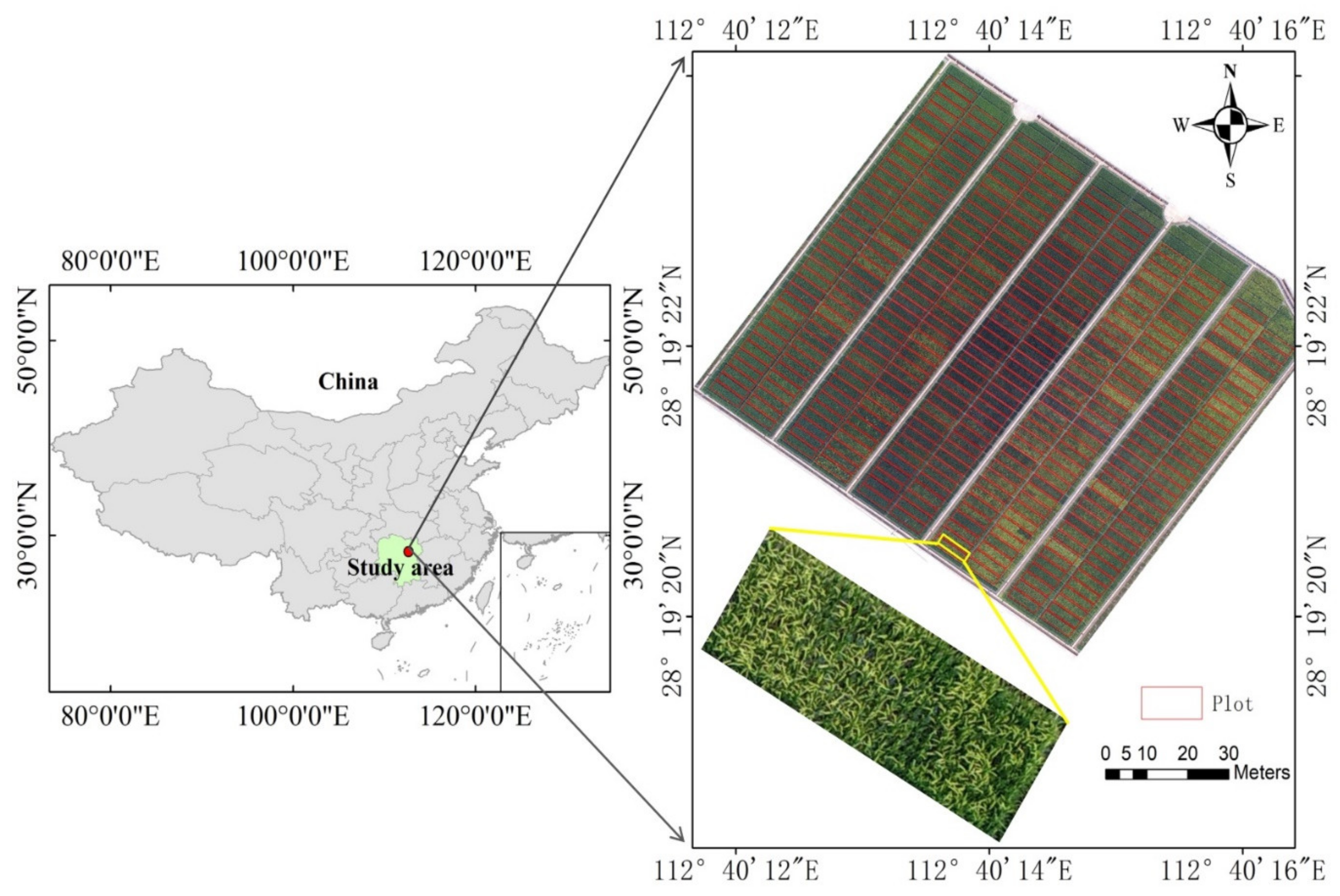
The experimental station is located at the Guanshan rice breeding base (28°19′ N, 112°40′ E), Jinzhou town, Ningxiang City, Hunan Province, China (Figure 1). Its annual average temperature, rainfall, and sunshine duration are 16.8 °C, 1358 mm, and 1739.2 h, respectively. The average annual sunshine hour duration per day is about 4.8 h. The soil type is fine-loam with pH, organic carbon, and total nitrogen concentrations of 6.7, 17.1 g kg−1, and 1.76 g kg−1, respectively.
In this study area, the breeding strategies include the photoperiod/thermo-sensitive genic male sterile line-based two-line system and the cytoplasmic male sterile line-based three-line system. A total of 122, 127, and 105 one-season-late indica hybrid rice combinations were investigated, respectively, in 2017, 2018, and 2019. These hybrids were developed by different breeding institutes and companies and were applied for commercial release in Hunan province, China. All hybrids were grown in a randomized complete block with three replicates. Seedlings were transplanted in each plot, which was comprised of 450 plants at spacing of 17 cm × 20 cm. All the experimental plots applied the same fertilizer treatment with N (195 kg ha−1), P2O5 (112 kg ha−1), and K2O (112 kg ha−1), using urea as the N fertilizer. The N fertilizer was split into three applications, with 40% being basal fertilizer, 40% being tillering fertilizer, and 20% being ear fertilizer. All phosphorus and potassium fertilizer were used as basal fertilizer. Water, insects, weeds, and disease were controlled when needed. Sowing was conducted in early June; then, transplanting was performed in late June or early July, depending on the climate conditions and seedling growth status (Table 1).
2.2. Field Data Collection
In field survey, rice breeders observed and recorded the growth stages of different cultivars every day; the phenological traits have been specifically described by Fageria et al. [38]. The basic phenological information of different rice cultivars were shown in Table 1 and Table A1. The rice grain yield of the investigated plots was harvested, depending on the maturity date of each rice cultivar. After the harvest, the grains were put into an oven at 75 °C until their weights did not change (after 72 h) and were then weighed by an electronic balance (±0.1 g).
To analyze the phenological differences among the rice cultivars from these plots, the duration and effective accumulated temperatures between the ST (sowing to transplant), TI (transplant to initial heading), IH (initial heading to full heading), HM (full heading to maturity), and SM (sowing to maturity) were calculated (Table A2). The effective accumulated temperature was calculated as follows:
where is the effective accumulated temperature, °C; where i = 1, 2, 3, … m days during the growing season. is the daily average temperature, °C; is the minimum temperature required for crop growth, °C. is the daily maximum temperature, °C; is the daily minimum temperature, °C. The biological upper limit temperature of rice () is 40 °C, and the lower limit temperature () is 10 °C [39].
2.3. UAV Data Acquisition and Image Processing
The UAV used in this study was a four-rotor consumer UAV (Phantom 4 Pro, SZ DJI Technology Co., Ltd., Shenzhen, China) with a maximum payload capacity of 1.375 kg. This UAV had a 1-in CMOS 20-megapixel camera mounted on its platform that was employed to capture the rice canopy images during the flights. Autonomous flights were carried out by Pix4Dcapture software to have overlap (70% forward and 80% side). The angular field of view is 60° horizontal × 27° vertical, resulting in a nominal resolution of 3.68 cm ground sampling distance (GSD) at 100 m above ground level. The focal length of the camera lens was 35 mm, and the RGB sensor could acquire 5456 × 3632 pixels over a brief period (faster than 1/2000 s). The captured camera images were in JPEG format. The images were collected on 6 September 2017; 7 September 2018; 29 August 2019, when practically all the rice cultivars were at the heading stage. The flights were carried out between 11:00 a.m. and 1:00 p.m. in stable ambient light conditions [9].
After the flights, the RGB images were downloaded from the memory card. The Pix4Dmapper (version 1.1.38, Pix4D SA, Lausanne, Switzerland) was used for image stitching. First, the overlapping images were automatically aligned by a feature point matching algorithm. Second, fifteen GCPs were used to georeference each image. Finally, the orthomosaic map with a TIFF image format was exported. In this study, VIs or bands were extracted from the orthomosaic maps by using the “GDAL” module in Python 3.6. Region of interests (ROIs) in individual plots were determined based on the orthomosaic maps by dividing the study area into regular plot polygons (Figure 1). In this study, Esri ArcGIS 10.2 software was used to draw ROIs and establish a buffer between boundary plots to reduce plot edge effects [40]. Then, the mean VI (Table 2) of ROI represented the value of each plot.
2.4. RF Model
RF is an ensemble learning method that combined the independent predictor results with bagging and random feature selection; the final result is obtained by voting or taking the mean value [48]. RF is insensitive to collinearity among multiple variables, obtaining high estimation accuracy and minimizing overfitting phenomenon [49].
In this study, fourteen VIs were calculated as different mathematical combinations of the three visible bands (i.e., red, green, and blue) from the UAV-based images (Table 2). Most of the VIs selected in this study were widely used to estimate the vegetation’s diverse biophysical parameters, such as aboveground biomass [50,51], chlorophyll content [52], nitrogen accumulation [9], and yield [41]. The phenological data involved five duration length variables (e.g., ST, TI, IH, HM, and SM) and five effective accumulated temperature variables (e.g., GDDST, GDDTI, GDDIH, GDDHM, and GDDSM) under specific growth stages (Table A2). The RF regression technique was carried out to establish the estimation model for grain yield in the breeding trial by using VIs only, phenological data only, and combination of VIs and phenological data. We used the dataset in 2017 and 2018 to train RF models. The remaining dataset in 2019 was used to test the RF models. Three hyperparameters that need to be tuned in an RF model are the maximum depth of trees (max_depth), minimum number of samples to split an internal node (min_samples_split), and minimum number of samples at a leaf node (min_samples_leaf). A grid search algorithm with 10-fold cross validation was used to split the set cultivar-wise in the calibration dataset to obtain optimal parameters values (Table 3). RF models were implemented by using the function “RandomForestRegressor” in the package of scikit-learn (https://scikit-learn.org/stable/, accessed on 28 November 2021) in Python 3.6.
2.5. CERES-Rice Model
2.5.1. Input Data
The input data for the CERES-Rice model included meteorological data, soil characteristics, field management information, and cultivar specific parameters. The meteorological data were collected from the local experiment meteorological station. The minimum requirement of weather data included daily maximum air temperature (°C), minimum air temperature (°C), solar radiation (MJ m−2 d−1), and precipitation (mm). The soil parameters and characteristics are shown in Table 4. The physical and chemical properties of each horizon of collected soil samples (Table 4) were analyzed by using the Soil Science Society of America (SSSA) and American Society of Agronomy (ASA) methods for soil analysis [53]. Field management information, such as planting date, transplanting date, harvest date, and fertilization amount, were shown in Table 1, Table A1, and Section 2.1. There are eight cultivar parameters in the CERES-Rice model: four phenology-related parameters (P1, P2R, P5, and P2O) and four yield-related parameters (G1, G2, G3, and G4). The cultivar parameters were determined by the generalized likelihood uncertainty estimation (GLUE) method. The specific procedures of parameter estimations were described in the following section.
2.5.2. Cultivar Parameter Estimations
In this study, we screened out 21 rice cultivars that were planted continuously over three years. The datasets in 2017 and 2018 were used to calibrate cultivar parameters. Then, the dataset in 2019 was used to evaluate the performance of the CERES-Rice model. The GLUE method exploited prior distributions of the parameters and variables to obtain the optimal value. First, Monte Carlo sampling of distributions were used to generate 6000 random parameter sets in each cultivar. Second, the likelihood value was calculated based on the mean observation data such as flowering date, maturity date, and grain yield. Then, we ran the CERES-Rice model 6000 times, and the results were evaluated by GLUE. After applying this approach to parameter sets, a final set of cultivar parameters was determined (Table A3).
2.6. Statistical Methods
The Pearson correlation analysis between studied variables and measured yield was carried out by a function called “pearsonr” in the Python module “scipy.stats”. A paired-samples t-test at p ≤ 0.05 was used for paired mean difference comparisons between the estimated values of the optimal RF model and the CERES-Rice model for 21 replicated cultivars across the years. The paired-samples t-test method was used to test the null hypothesis “there were no significant differences in the predictions of the optimal RF model and CERES-Rice model for 21 replicated cultivars in 2019”. The normality of the distribution of sample datasets was tested by using the Kolmogorov–Smirnov test, and homogeneity of variances was tested by using the Levene test. All sampled datasets followed a normal distribution (p-values > 0.05) and similar variances (p-values > 0.05). Therefore, a paired-samples t-test could be used in this research. The Python script named “ttest_rel” function from Scipy Python module was used to perform the paired-samples t-tests.
For yield estimation, the performance of models was evaluated in the calibration dataset (in 2017 and 2018) and validation dataset (in 2019), respectively. The estimation accuracy of the yield model was quantified using the coefficient of determination (R2, Equation (2)), root mean square error (RMSE, Equation (3)), and mean absolute error (MAE, Equation (4)). These statistical indices were calculated as follows:
where is the number of samples in the calibration or validation data set; is the estimated yield; is the measured yield; is the mean value of the measured yield. Mathematically, the model with higher values of R2, a smaller RMSE and MAE corresponds to more accurate results.
3. Results
3.1. Statistical Analysis of Measured Yield
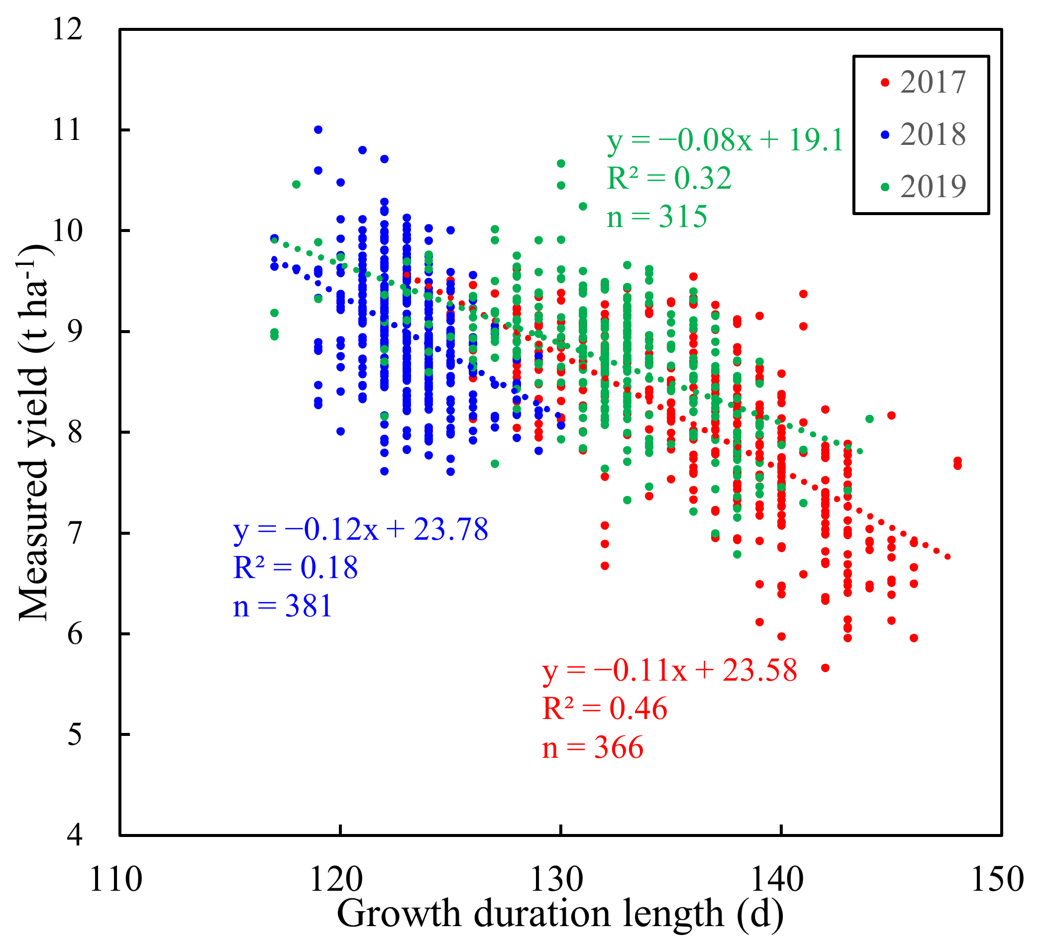
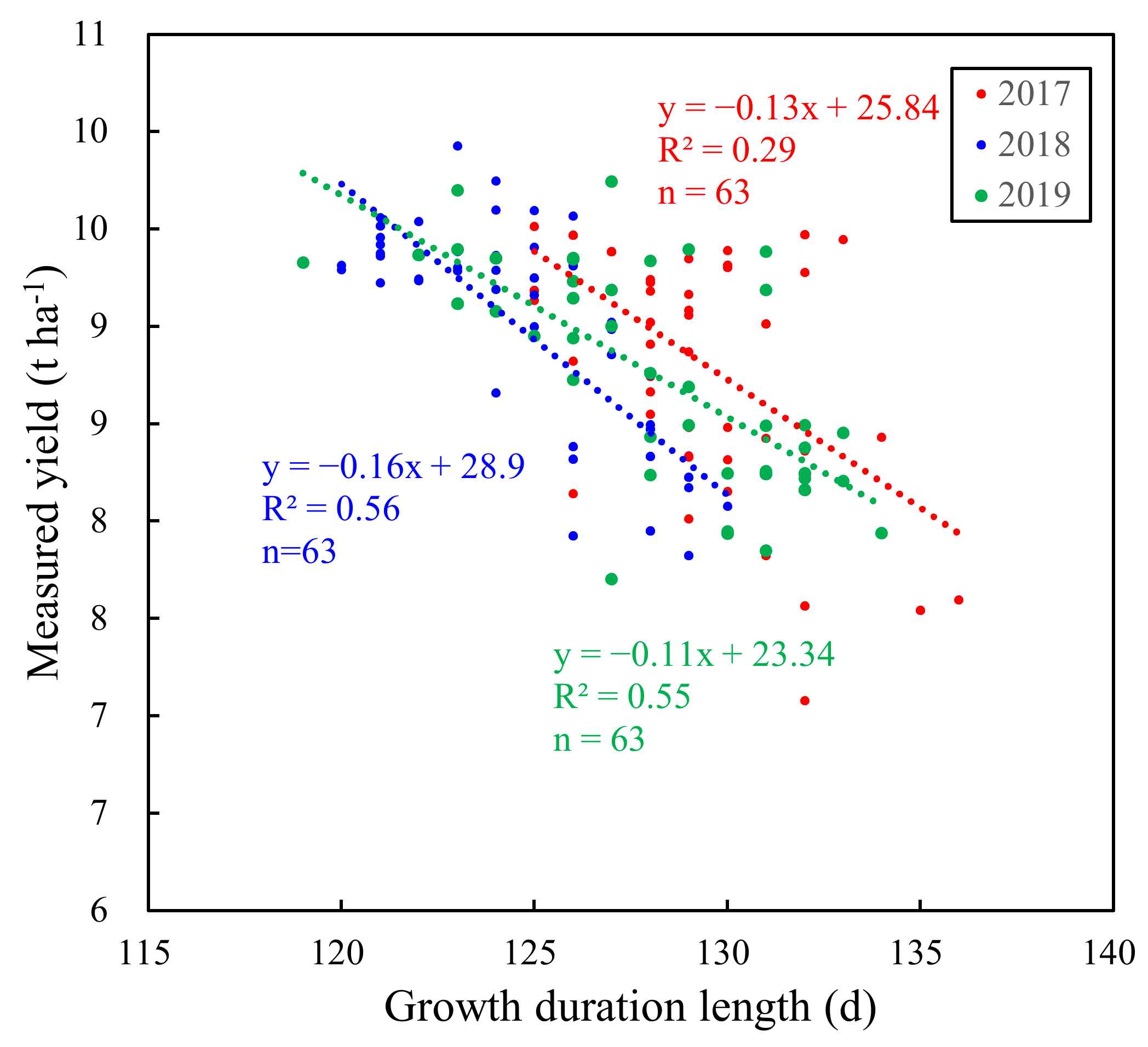
Figure 2 shows the negative correlations between the yield and the growth duration length from sowing to maturity (GDL) for all cultivars in 2017, 2018, and 2019. Strong correlations were observed between yield and GDL in 2017 and 2019. The linear correlation between yield and GDL seemed slightly weak in 2018. Figure 3 also shows negative correlations between yield and GDL for 21 replicated cultivars across the years. The variability of yield was larger than that of GDL for all cultivars, as well as for 21 replicated cultivars across the years (Table 5). Note that the GDL of cultivars in 2018 tended to be smaller than that in 2017 and 2019. The GDL difference was largely attributed to the variations in climate conditions across the years. The mean daily temperature between sowing and maturity in 2018 was 1.4 °C and 0.7 °C higher than that in 2017 and 2019, respectively (Table A4). Additionally, the mean values of yield for 21 replicated cultivars were relatively consistent across the years.
3.2. Analysis of VIs and Phenological Data
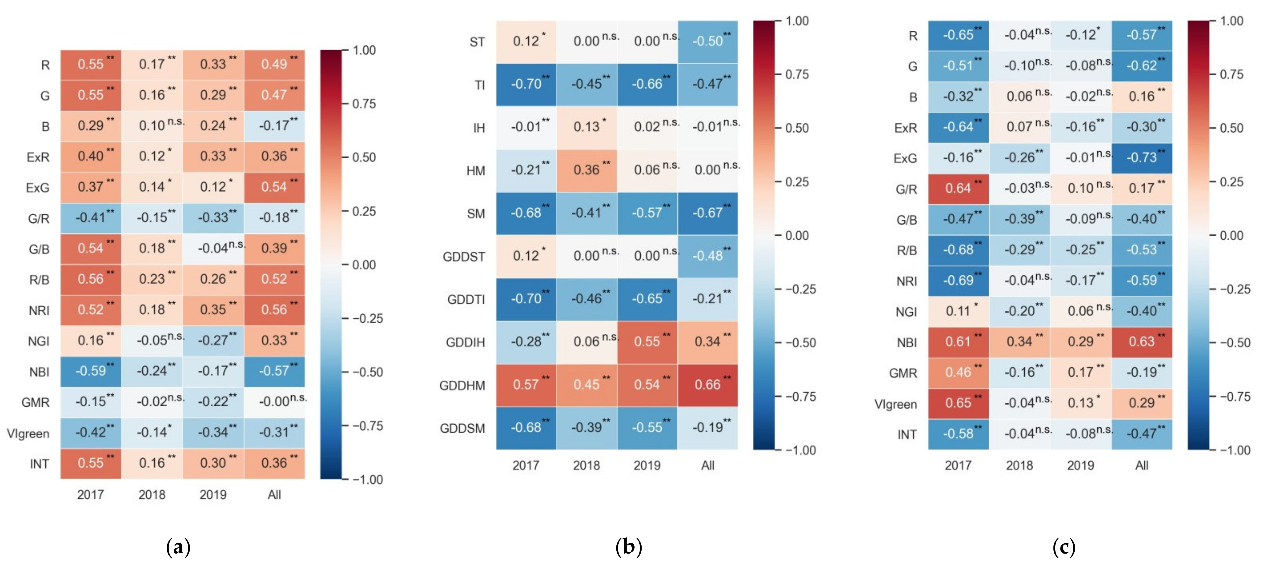
Figure 4a,b show the Pearson correlation coefficients between VIs and phenology and yield. The correlation between VIs and yield was somewhat inconsistent in different years. Generally, all VI variables were significantly correlated (p < 0.05) with the measured yield in 2017. However, most VIs in 2018 and 2019 were weakly correlated with yield. For example, the largest absolute values of Pearson coefficients (|r|) were only 0.24 and 0.35 in 2018 and 2019, respectively. Conversely, the correlation between phenology and yield was relatively consistent across the years. For example, the two growth duration length variables (TI and SM) and one effective accumulated temperature (GDDHM) had a strong correlation with yield (|r| ranged from 0.41 to 0.70, p < 0.01) in different years and combined years. Some phenological variables such as ST, IH, HM, and GDDST had weak or no significant correlation (p > 0.05) with yield across the years. Figure 4c shows the relationship between VIs and GDL. All VI variables were significantly correlated with GDL (p < 0.05) in 2017. However, some VI variables such as G, B, G/R, and INT had no significant correlation with GDL (p > 0.05) in 2018 and 2019. Accordingly, the relationship between VIs and GDL was inconsistent across the years.
3.3. RF Method for Yield Estimation
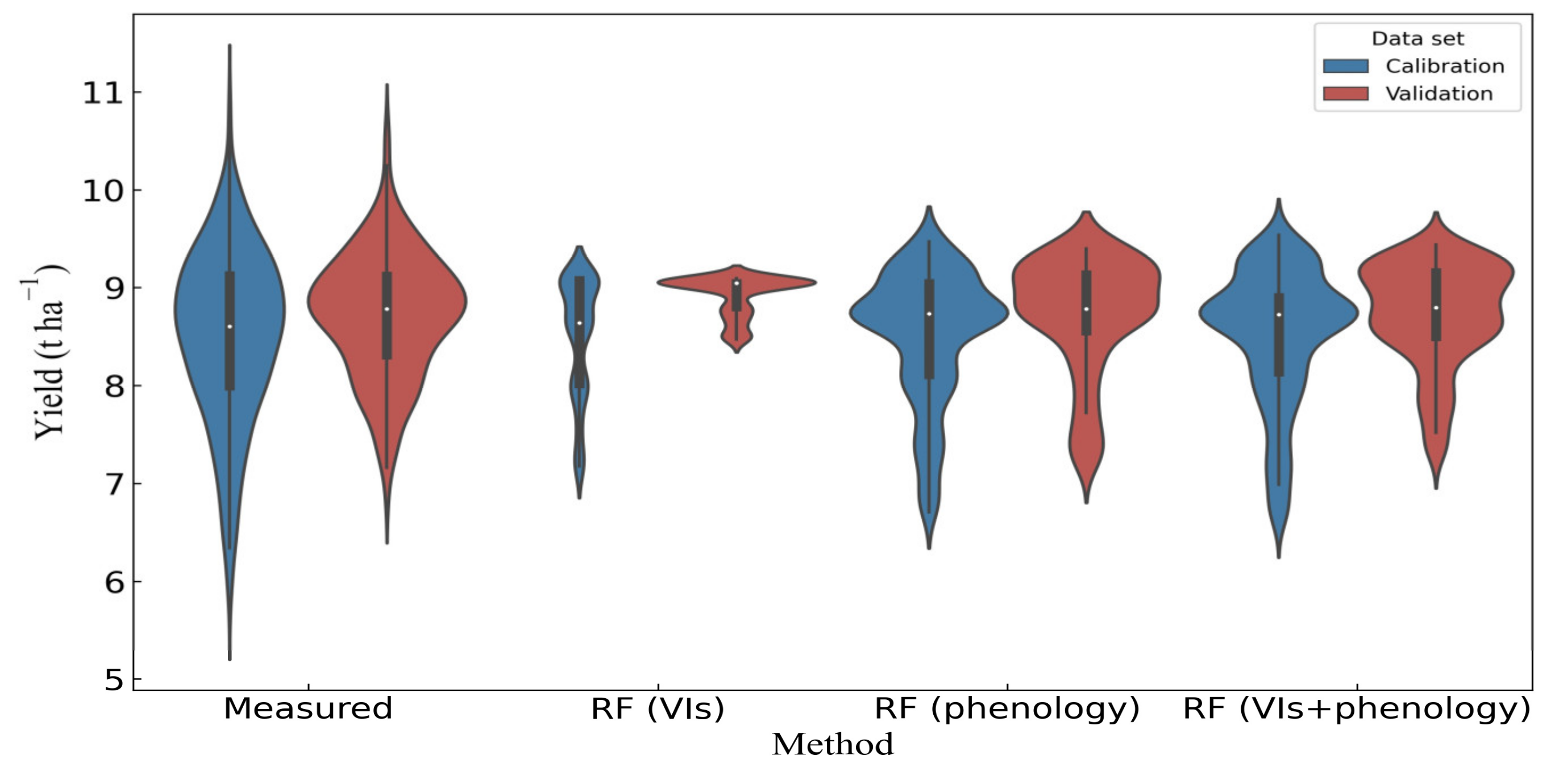
Three different RF models were established for yield estimation in rice breeding, and the results were evaluated using R2, RMSE, and MAE. Figure 5 shows the distributions of the simulated yield by those models in calibration and validation sets. When using VIs only as inputs, the simulated yield based on the RF model was mainly around 9 t ha−1. The variation of simulated yield was small, especially in the validation dataset (Figure 5). When using phenology data as inputs, the distribution of simulated yield was similar to that of the RF (VIs + phenoloy) model. The range of simulated yield in the RF (VIs + phenoloy) model was closer to the range of the measured yield. However, all the RF models underestimated yield at the high yield level, to a certain extent.
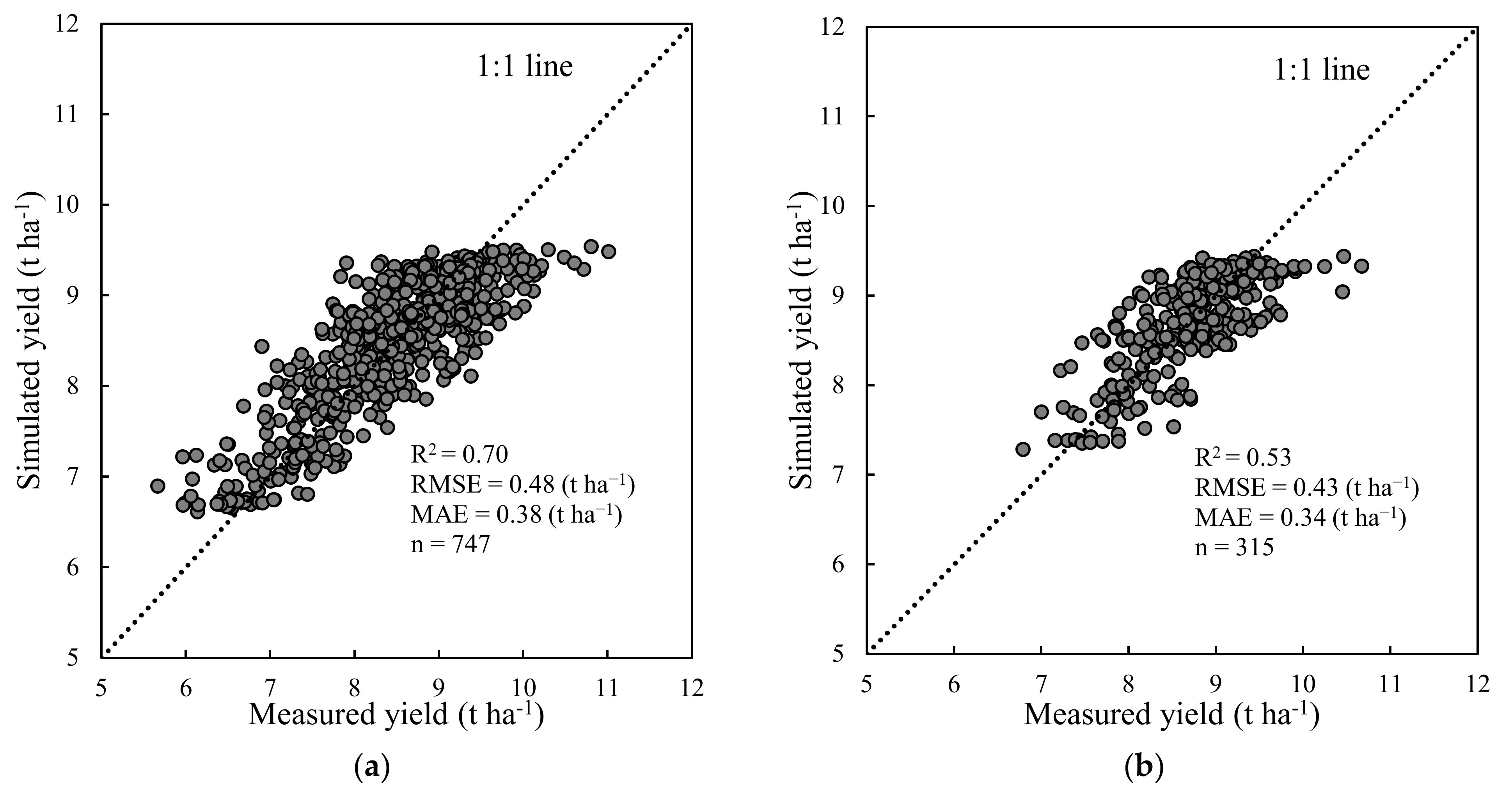
In comparison with approaches that solely use VIs or phenology to estimate rice yield, the RF (VIs) model exhibited unsatisfactory performance for yield estimation in the validation set with R2 = 0.06, RMSE = 0.65 t ha−1, and MAE = 0.51 t ha−1, respectively. In contrast, the RF model that used only phenological data exhibited good yield estimations with R2 values of 0.62 and 0.46 in the calibration and validation sets, respectively, which indicated that the phenological information across rice cultivars was an important factor in determining yield in rice breeding. When combined RGB–VIs and phenological data as inputs, the RF model (VIs + phenology) achieved the highest performance in rice yield estimation in the calibration and validation sets; R2, RMSE, and MAE were 0.70 and 0.53, 0.48 and 0.43 t ha−1, and 0.38 and 0.34 t ha−1, respectively (Table 6). These results indicated that more variables in the RF model provided more accurate yield estimation. However, the RF (VIs + phenology) model in the all datasets underestimated the yield when the measured yields were greater than 10 t ha−1 (Figure 6). Additionally, the optimal RF model overestimated yield when the measured yields were less than 7 t ha−1 (Figure 6).
3.4. CERES-Rice Model for Yield Estimation
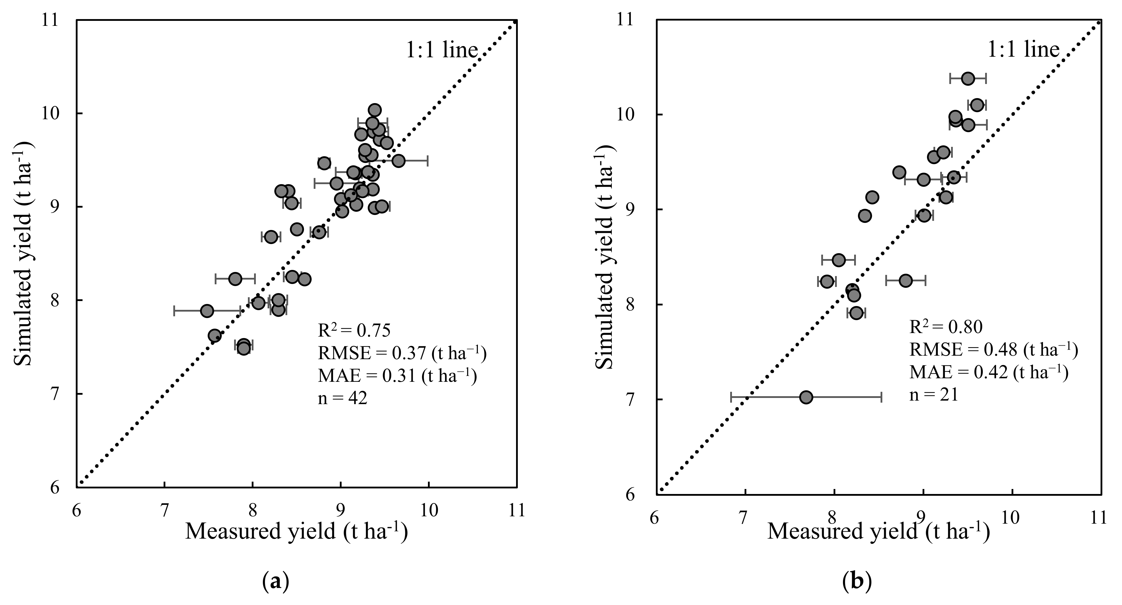
Unlike the RF regression technique for yield estimation proposed in Section 2.4, the CERES-Rice model is a crop growth dynamic model that can simulate yield, aboveground biomass, crop phenology, etc. Based on the dataset of 21 rice cultivars planted over three years in the experimental site, the GLUE method was used to obtain 21 sets of rice cultivar parameters (Table A3). The relationship between the simulated and measured yield was shown in Figure 7. The result showed the good accuracy with the R2, RMSE, and MAE values of 0.75 and 0.80, 0.37 and 0.48 t ha−1, and 0.31 and 0.42 t ha−1 in calibration set and validation set, respectively. The accuracy of CERES-Rice model for yield estimation was slightly better to that of deep convolutional neural networks for rice yield estimation with R2 and RMSE values of 0.59 and 0.66 t ha−1, respectively [27]. These results indicated that the yield from the CERES-Rice model provided relatively accurate estimations.
3.5. Performance Comparison between CERES-Rice Model and the Optimal RF Model
In order to evaluate the robustness and capacity of the optimal RF model that combined VIs and phenological data as inputs, the simulated yield of the 21 rice cultivars planted over three years based on the RF (VIs + phenology) model was compared with that of the CERES-Rice model. Figure 8 shows the relationship between the measured yield and simulated yield obtained from these two models. Compared to the RF (VIs + phenology) model, the slope and R2 values of the linear regression between simulated yield, based on the CERES-Rice and measured yield, were closer to 1. However, the values of RMSE and MAE, based on the optimal RF model, were comparable to those based on the CERES-Rice model (Table 7). In addition, the paired-sample t-tests results showed that there were no significant differences between the CERES-Rice model and the optimal RF model for simulated yields in 2019 (p > 0.05, Table 7).
4. Discussion
4.1. Response of Phenology to Yield
Phenology determines the amount of interception of solar radiation by the rice canopy that is closely associated with grain yield [34]. In this study, 10 phenological indicators were selected to analyze their correlation with yield. It was found that the GDDHM, TI, and SM were significantly correlated (|r| > = 0.41, p < 0.01) with the yield for each year and combined years (Figure 4b). Among the three phenological indicators, GDDHM was positively related to yield across the years (r > = 0.45, p < 0.01). This result is supported by the previous study, which found that GDDmat (from 50% heading to maturity) was positively associated with yield (r = 0.46) in Italian rice germplasm [54]. In our study, the mean daily temperatures during the reproductive period were in the optimum temperature range (20–35 °C) for rice development (Table A4) [55]. The increase in mean daily temperature during this phase could increase GDDHM significantly and then increase the photosynthesis rate, which contributes to rice yield increase [56]. The strong negative relationship was found between TI and yield across the years (r from −0.45 to −0.70, p < 0.01), suggesting that the cultivars with short durations before heading presented a high-level yield. One possible explanation is that cultivars with short durations during the vegetative phase could reduce N uptake to ensure N supply at the reproductive phase, which is beneficial to increase the yield. However, due to the limitations of the observed data, we could not provide any qualitative or quantitative explanation; the relationship among N uptake, duration length, and yield needs to be further studied in rice breeding. The short GDL (i.e., SM) tended to afford high grain yield in the Guanshan rice breeding base (Figure 2), which was consistent with the results by using short growth durations in central China [57]. They found that the grain yield improved by way of desirable traits, e.g., the plants were tall, and the panicles were heavy. Chen et al. [58] also demonstrated that short-duration cultivars had higher spikelet filling rate and higher harvest index than long-duration cultivars in Hunan Province, China; thus, the higher grain yield could be a target for breeding high-yielding rice cultivars with short durations. Climate warming has reduced the rice growth duration in China over the past three decades [59]; short-duration cultivars were proposed for German oats without the stress caused by climate warming [60]. It needs to be pointed out that, despite certain associated yield penalties, the use of short-duration cultivars could be a viable option for adaptation to climate change. Cultivating short-duration cultivars may be beneficial to rice yields by avoiding extreme heat stress at the heading stage (i.e., flowering) [61] and reducing drought exposure [62]. In the long run, the yield benefits brought by the positive shifts of cultivar traits may offset the losses caused by the adverse phenological changes to a certain extent [59]. However, in this study, we only analyzed the relationship between phenology (i.e., GDL and effective accumulated temperature variables) and yield, and we did not try to quantify the decline in yield due to the increase of GDL because pest and disease pressure, a variety of genetic properties such as spikelet fertility and the harvest index are equally important for determining the yields. Since rice breeding depends on both consumer demands and climate in China, further research is necessary to be carried out to determine the reasons for the improved performance of short-duration cultivars by combining measured data or obtaining information that could reflect rice breeding objectives.
4.2. Importance of Phenology to RF Model Formulation
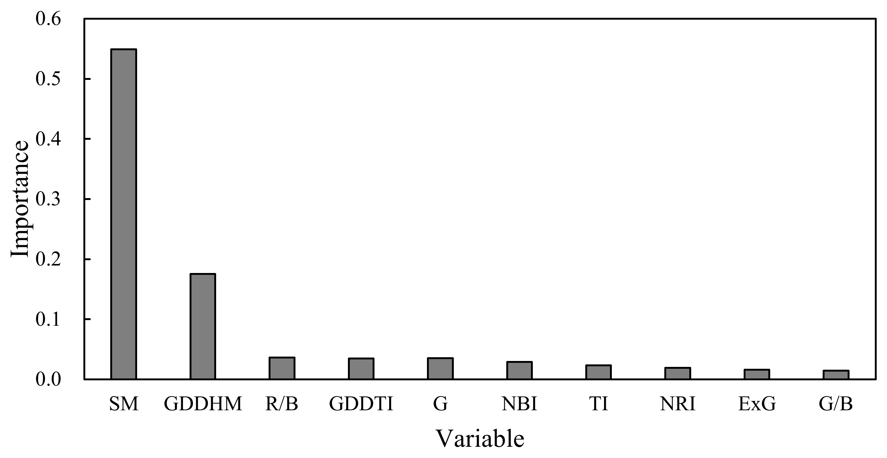
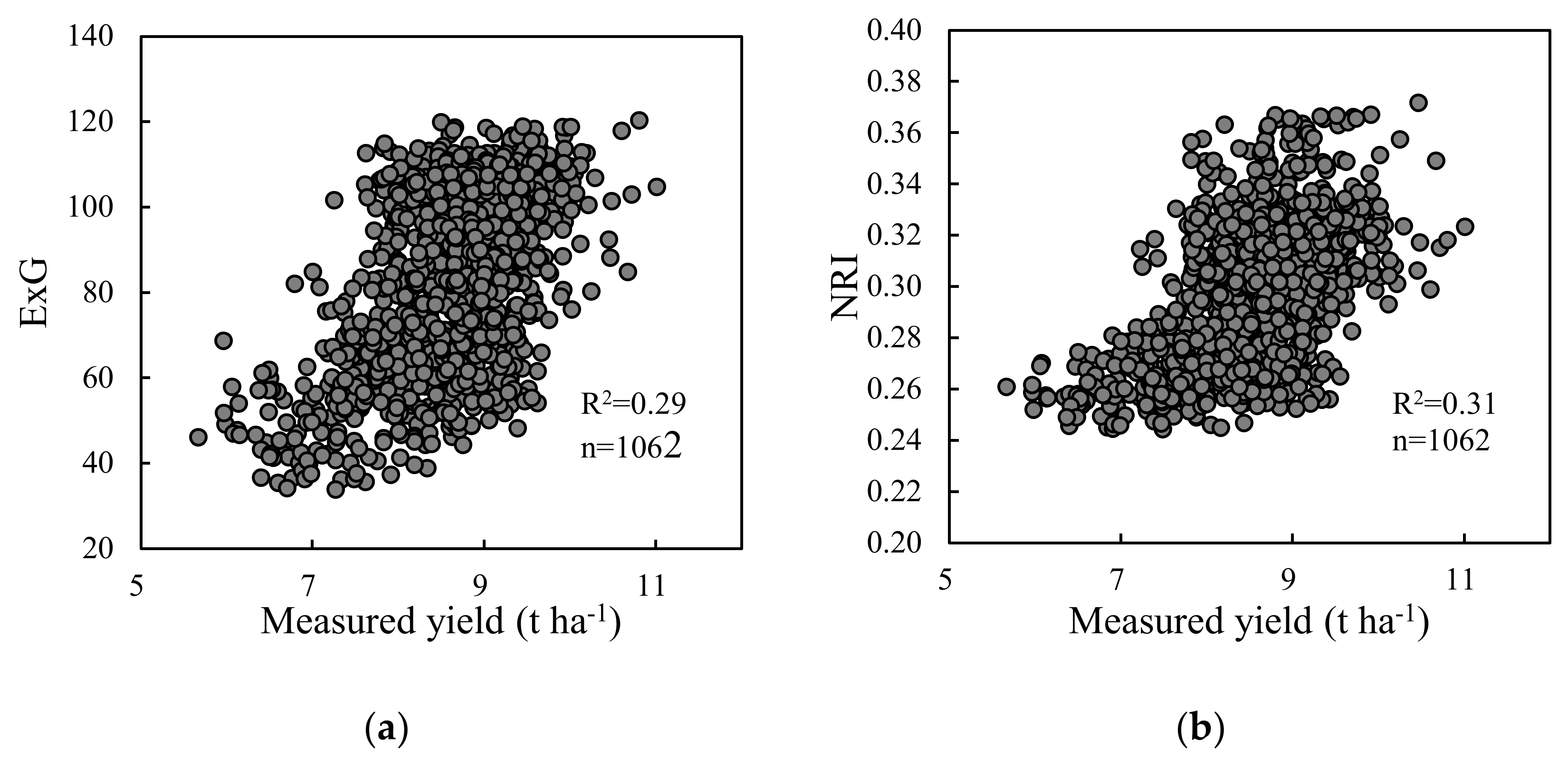
At present, the ability to estimate crop yields based on UAV images is an area of active research [63]. The applications of VIs obtained from UAV images, such as NDVI, E × G, and VIgreen, have been reported in rice yield predictions [36,63]. However, there are few studies describing yield estimation based on the UAV-VIs in rice breeding. In this study, the relationships between yield and VIs from UAV-RGB images were analyzed from 2017 to 2019. In terms of variable importance, R/B was the most important for yield estimation in the optimal RF model among the 14 VIs (Figure 9). This was mainly attributed to the consistent performance of R/B on yield across the years (Figure 4a). However, the RF model based on only VIs had an insufficient accuracy and over-fitting problems for yield estimation (Table 6 and Figure 5). There were three main reasons for these results: (1) the variation in Pearson correlation between VIs and yield was relatively large and inconsistent across the three years (Figure 4a); (2) due to the high vegetation coverage at the heading stage, VIs (e.g., E × G and NRI) became obviously saturated (Figure A1), and this result was consistent with the findings of Zhou et al. [63] and Gitelson et al. [64]; (3) the effect of VI values on yield was barely quantified because of the variation in the phenology across cultivars in rice breeding. Compared with the RF model using VIs only, adding phenology significantly improved the accuracy of yield estimation (Table 6). Significant benefits were associated with the use of phenological information and VIs in the remote sensing-based soybean and maize yield models [65], which were similar to the results of this study. Yang et al. [27] also pointed out that the combination with the observations of phenological dates could improve model accuracy for yield estimation. In this study, the phenological variables, such as SM and GDDHM, had the determined effect on model estimation accuracy in rice breeding (Figure 9). We demonstrated that phenological data dominated the yield variance, and the data set of VIs provided the secondary contribution to yield estimation. However, the phenological stages of plots were based on manual observation in the experimental site. Recently, the VI data have been widely used to extract phenology. The methodologies based on VI data are mainly shown as two types: (1) curve fitting methods that used Savitzky-Golay filtering, logistic function, and Gaussian function to smooth the time-series VI curves, then extracted phenological information based on its inflection points [66,67]; (2) shape model fitting methods that could smooth VI curves, and then extracted phenology based on optimum scaling coefficients and visual observations [68]. These methodologies based on time-series VI data often relied on high temporal resolutions. Therefore, it was necessary to detect phenology-based on time-series images from UAV to improve the applicability of the RF models for yield estimation in the future.
4.3. Comparison between RF and CERES-Rice Models
There were no significant differences in the estimated yield (p > 0.05) between the optimal RF model and the CERES-Rice model based on the paired-samples t-tests (Table 7). The accuracy of estimated yield in these two models was comparable in terms of RMSE and MAE. In fact, the statistical assumptions of these two kinds of models were totally different. The CERES-Rice model was a process-based model that required advanced data in higher costs. In this study, 21 replicated rice cultivars planted for three years were selected to simulate yield by using the CERES-Rice mode. Although, the crop growth model could obtain reliable and satisfactory results in agriculture [19,20,21]. Using crop growth models to simulate yield for breeding programs is still challenged by the variances in phenotypes and genotypes. It is difficult for crop growth models to calculate cultivar parameters in hundreds and even more breeding materials. In contrast, the RF model proposed in this paper, with the use of UAV-based RGB images, was performed at the decreased cost. The simulation results based on the optimal RF model coincide with the measured yield (Figure 10). In this study, the optimal RF model could be used as a case to prove that the fusion of VIs and phenological data in an RF model were useful and promising for yield estimation in breeding. Similar conclusions could be found in the study of Wan et al. [36], where they found that the fusion of VIs and crop traits in an RF model could improve model accuracy for yield estimation. However, yield was affected by many factors such as crop traits, environmental conditions (heat stress and cold stress), and field management [51,54,55], which made the RF model difficult to apply for large areas. Thus, the feasibility of estimating yield in the field by using phenological data and VIs from high-resolution UAV images should be additionally determined by the more field validation. Future studies are also required to verify the use of phenology and VIs for different ecological areas and crops.
There were some limitations for the RF models to further improve the yield estimation accuracy. For example, the images of multi-growth stages needed to be examined for yield estimation. There were only three bands (R, G, and B) of images used to calculate VIs. Thus, the spectral information of multispectral and hyperspectral sensors mounted on UAS should be captured and further analyzed. In addition, other methodological methods such as machine learning (ML) and deep learning might be applied to improve yield estimation accuracy in rice breeding.
5. Conclusions
In this study, 14 VIs derived from UAV-based images and phenological data were used to estimate grain yield in rice breeding from 2017 to 2019. Three RF models based on VIs and phenological variables were constructed for yield estimation. The results demonstrated that these models explained 52–70% and 6–53% of grain yield variability, respectively, in calibration and validation sets. VIs from the UAV–RGB imagery had inadequate performances in yield estimation because of differences in phenology across rice cultivars. The RF model that combined VIs and phenological data obtained the best accuracy for yield estimation. Further analysis indicated that phenology dominated the yield variance, and VIs provided a secondary contribution to the estimation of yield in rice breeding. Additionally, there were no significant differences between the simulated yields of the optimal RF model and the CERES-Rice model for 21 replicated cultivars. These results further indicated that the foregoing RF model demonstrated the considerable potential for yield estimation in rice breeding. Future work should be carried out to investigate the RF model with spectral information derived from the multispectral and hyperspectral sensors onboard UAS in multiple growth stages to improve the model robustness and applicability.
Author Contributions
Conceptualization, H.G.; methodology, H.G.; investigation, C.D., H.G., F.M., and Z.L.; resources, C.D.; data curation, H.G.; writing—original draft preparation, H.G.; writing—review and editing, C.D.; visualization, H.G.; supervision, C.D. All authors have read and agreed to the published version of the manuscript.
Funding
This study was supported by the Key Research and Development Program of Shandong Province (2019JZZY010713), National Key Research and Development Program of China (No. 2018YFE0107000), and the National Natural Science Foundation of Jiangsu Province (BK20191110).
Data Availability Statement
Data sharing not applicable.
Acknowledgments
Thanks to Jingyou Guo and Youdong Hu for providing the details of the experimental design in this study.
Conflicts of Interest
The authors declare no conflict of interest.
Appendix A

Table A1.
Statistics of phenological dates after transplanting across rice cultivars.
| Year | Plots | Cultivars | Initial Heading Date | Full Heading Date | Maturity Date |
|---|---|---|---|---|---|
| 2017 | 366 | 122 | August 25–September 15 | August 31–September 19 | October 8–December 2 |
| 2018 | 381 | 127 | August 19–September 5 | August 23–September 9 | October 5–October 17 |
| 2019 | 315 | 105 | August 15–September 3 | August 20–September 8 | October 1–October 28 |
Table A2.
Basic information of phenology across rice cultivars from 2017 to 2019.
| Descriptive Statistics | Duration length (d) | Growth Degree Days (°C) | ||||||||
|---|---|---|---|---|---|---|---|---|---|---|
| ST | TI | IH | HM | SM | GDDST | GDDTI | GDDIH | GDDHM | GDDSM | |
| Min | 19 | 47 | 3 | 34 | 117 | 358 | 990 | 59 | 412 | 2061 |
| Max | 32 | 68 | 7 | 56 | 148 | 521 | 1412 | 140 | 720 | 2329 |
| Mean | 24.03 | 58.99 | 4.55 | 42.83 | 130.40 | 419.64 | 1211.13 | 97.10 | 560.11 | 2233 |
| SD | 5.76 | 3.91 | 0.55 | 3.44 | 7.08 | 72.55 | 77.03 | 17.69 | 62.45 | 35.86 |
| CV (%) | 23.96 | 6.63 | 12.16 | 8.02 | 5.43 | 17.29 | 6.36 | 18.22 | 11.15 | 1.61 |
Note: ST, duration (days) from sowing to transplant; TI, duration (days) from transplant to initial heading; IH, duration (days) from initial heading to full heading; HM, duration (days) from full heading to maturity; SM, duration (days) from sowing to maturity; GDDST, GDDTI, GDDIH, GDDHM, and GDDSM represent effective accumulated temperatures (°C) for ST, TI, IH, HM, and SM, respectively.
Table A3.
Cultivar coefficients of rice varieties used in the CERES-Rice model.
| Cultivar Name | P1 | P2R | P5 | P2O | G1 | G2 | G3 | G4 |
|---|---|---|---|---|---|---|---|---|
| 5960You058 | 665 | 285.7 | 518.1 | 12.72 | 51.81 | 0.026 | 1.187 | 0.954 |
| CLY343 | 706.2 | 190.6 | 445.2 | 11.96 | 51.32 | 0.022 | 1.231 | 0.991 |
| R534 | 591.1 | 169 | 491.2 | 11.11 | 51.73 | 0.022 | 1.079 | 1.001 |
| HYY605 | 612.9 | 221.6 | 491.7 | 12.78 | 67.41 | 0.025 | 1.134 | 0.943 |
| HLY2035 | 275 | 278.2 | 422.7 | 11.27 | 55.6 | 0.021 | 1.265 | 0.8 |
| HLY3748 | 288.6 | 227.1 | 483.2 | 11.44 | 66.58 | 0.02 | 1.245 | 0.878 |
| HLY5035 | 565.7 | 249.5 | 432.4 | 12.09 | 58.46 | 0.022 | 1.239 | 1.019 |
| HLY7155 | 487.7 | 243.4 | 531.7 | 13.11 | 66.84 | 0.025 | 0.793 | 0.988 |
| HLY8210 | 418.9 | 259.5 | 483.3 | 13.57 | 73.89 | 0.025 | 0.729 | 1.059 |
| JLY1678 | 395.4 | 95.5 | 689.1 | 9.62 | 71.17 | 0.025 | 0.866 | 1.032 |
| JLY2626 | 395.4 | 75.1 | 454 | 7.544 | 66.38 | 0.024 | 1.257 | 1.043 |
| JLY9936 | 395.4 | 182.4 | 643.1 | 11.91 | 59.47 | 0.03 | 0.851 | 0.974 |
| LFY905 | 601.3 | 98.76 | 465.1 | 10.33 | 60.05 | 0.022 | 1.106 | 1.057 |
| LJY8246 | 555.8 | 130 | 409.9 | 10.05 | 50.04 | 0.024 | 0.85 | 1.006 |
| LLY3748 | 395.4 | 283.7 | 461.8 | 12.35 | 61.62 | 0.024 | 0.841 | 1.039 |
| LLY5809 | 395.4 | 76.56 | 450 | 7.133 | 59.89 | 0.025 | 1.263 | 1.077 |
| RLY1019 | 417.5 | 142.8 | 520 | 10.5 | 55.55 | 0.03 | 1.097 | 0.88 |
| WLY6018 | 395.4 | 60 | 472.7 | 3 | 71.52 | 0.025 | 1.196 | 0.957 |
| XLY7629 | 395.4 | 86.07 | 506.5 | 9.049 | 52.11 | 0.03 | 0.955 | 1.045 |
| XLY8736 | 395.4 | 330 | 550 | 12.94 | 61.46 | 0.03 | 1.244 | 0.907 |
| YLY526 | 601.3 | 193.2 | 450 | 11.52 | 55.44 | 0.024 | 0.966 | 0.898 |
Note: P1 represents juvenile phase coefficient, GDD; P2R represents photoperiodism coefficient, GDD; P5 represents grain filling duration coefficient, GDD; P2O represents critical photoperiod, h; G1 represents spikelet number coefficient; G2 represents single grain weight, g; G3 represents tillering coefficient; G4 represents temperature tolerance coefficient.
Table A4.
The mean daily temperature (), minimum temperature () and maximum temperature () during different growth stages from 2017 to 2019.
Table A4.
The mean daily temperature (), minimum temperature () and maximum temperature () during different growth stages from 2017 to 2019.
| Year | ST | TI | IH | HM | SM | ||||||||||
|---|---|---|---|---|---|---|---|---|---|---|---|---|---|---|---|
| 2017 | 23.4 | 29.2 | 26.3 | 26.6 | 33.8 | 30.2 | 22.1 | 26.8 | 24.5 | 19.3 | 25.7 | 22.5 | 23.4 | 30.0 | 26.7 |
| 2018 | 24.8 | 32.7 | 28.8 | 26.7 | 34.5 | 30.6 | 25.4 | 30.7 | 28.0 | 20.6 | 28.0 | 24.3 | 24.3 | 32 | 28.1 |
| 2019 | 23.0 | 30.1 | 26.5 | 26.4 | 34.4 | 30.4 | 25.2 | 30.8 | 28.0 | 20.4 | 27 | 23.7 | 23.7 | 31.1 | 27.4 |
Note: ST, duration (days) from sowing to transplant; TI, duration (days) from transplant to initial heading; IH, duration (days) from initial heading to full heading; HM, duration (days) from full heading to maturity; SM, duration (days) from sowing to maturity.
Figure A1.
Vegetation indices vs. measured yield; (a) ExG and yield; (b) NRI and yield. These two vegetation indices were Figure 4a.
Figure A1.
Vegetation indices vs. measured yield; (a) ExG and yield; (b) NRI and yield. These two vegetation indices were Figure 4a.

References
- Son, N.T.; Chen, C.F.; Chen, C.R.; Minh, V.Q.; Trung, N.H. A comparative analysis of multitemporal MODIS EVI and NDVI data for large-scale rice yield estimation. Agric. For. Meteorol. 2014, 197, 52–64. [Google Scholar] [CrossRef]
- Bastiaanssen, W.G.M.; Ali, S. A new crop yield forecasting model based on satellite measurements applied across the Indus Basin, Pakistan. Agric. Ecosyst. Environ. 2003, 94, 321–340. [Google Scholar] [CrossRef]
- Reynolds, C.A.; Yitayew, M.; Slack, D.C.; Hutchinson, C.F.; Huete, A.; Petersen, M.S. Estimating crop yields and production by integrating the FAO Crop specific Water Balance model with real-time satellite data and ground-based ancillary data. Int. J. Remote Sens. 2000, 21, 3487–3508. [Google Scholar] [CrossRef]
- Sakamoto, T.; Gitelson, A.A.; Arkebauer, T.J. MODIS-based corn grain yield estimation model incorporating crop phenology information. Remote Sens. Environ. 2013, 131, 215–231. [Google Scholar] [CrossRef]
- Inoue, Y.; Sakaiya, E.; Zhu, Y.; Takahashi, W. Diagnostic mapping of canopy nitrogen content in rice based on hyperspectral measurements. Remote Sens. Environ. 2012, 126, 210–221. [Google Scholar] [CrossRef]
- Yonezawa, C.; Negishi, M.; Azuma, K.; Watanabe, M.; Ishitsuka, N.; Ogawa, S.; Saito, G. Growth monitoring and classification of rice fields using multitemporal RADARSAT-2 full-polarimetric data. Int. J. Remote Sens. 2012, 33, 5696–5711. [Google Scholar] [CrossRef]
- Kern, A.; Barcza, Z.; Marjanovic, H.; Arendas, T.; Fodor, N.; Bonis, P.; Bognar, P.; Lichtenberger, J. Statistical modelling of crop yield in Central Europe using climate data and remote sensing vegetation indices. Agric. For. Meteorol. 2018, 260, 300–320. [Google Scholar] [CrossRef]
- Zhang, C.; Kovacs, J.M. The application of small unmanned aerial systems for precision agriculture: A review. Precis. Agric. 2012, 13, 693–712. [Google Scholar] [CrossRef]
- Zheng, H.; Cheng, T.; Li, D.; Zhou, X.; Yao, X.; Tian, Y.; Cao, W.; Zhu, Y. Evaluation of RGB, Color-Infrared and Multispectral Images Acquired from Unmanned Aerial Systems for the Estimation of Nitrogen Accumulation in Rice. Remote Sens. 2018, 10, 824. [Google Scholar] [CrossRef] [Green Version]
- Koppe, W.; Gnyp, M.L.; Hennig, S.D.; Li, F.; Miao, Y.; Chen, X.; Jia, L.; Bareth, G. Multi-Temporal Hyperspectral and Radar Remote Sensing for Estimating Winter Wheat Biomass in the North China Plain. Photogramm. Fernerkund. Geoinf. 2012, 3, 281–298. [Google Scholar] [CrossRef]
- Jin, X.; Yang, G.; Xu, X.; Yang, H.; Feng, H.; Li, Z.; Shen, J.; Zhao, C.; Lan, Y. Combined Multi-Temporal Optical and Radar Parameters for Estimating LAI and Biomass in Winter Wheat Using HJ and RADARSAR-2 Data. Remote Sens. 2015, 7, 13251–13272. [Google Scholar] [CrossRef] [Green Version]
- Peng, Y.; Zhu, T.e.; Li, Y.; Dai, C.; Fang, S.; Gong, Y.; Wu, X.; Zhu, R.; Liu, K. Remote prediction of yield based on LAI estimation in oilseed rape under different planting methods and nitrogen fertilizer applications. Agric. For. Meteorol. 2019, 271, 116–125. [Google Scholar] [CrossRef]
- Palosuo, T.; Kersebaum, K.C.; Angulo, C.; Hlavinka, P.; Moriondo, M.; Olesen, J.E.; Patil, R.H.; Ruget, F.; Rumbaur, C.; Takac, J.; et al. Simulation of winter wheat yield and its variability in different climates of Europe: A comparison of eight crop growth models. Eur. J. Agron. 2011, 35, 103–114. [Google Scholar] [CrossRef] [Green Version]
- Katerji, N.; Campi, P.; Mastrorilli, M. Productivity, evapotranspiration, and water use efficiency of corn and tomato crops simulated by AquaCrop under contrasting water stress conditions in the Mediterranean region. Agric. Water Manag. 2013, 130, 14–26. [Google Scholar] [CrossRef]
- Wang, X.; Liu, G.; Yang, J.; Huang, G.; Yao, R. Evaluating the effects of irrigation water salinity on water movement, crop yield and water use efficiency by means of a coupled hydrologic/crop growth model. Agric. Water Manag. 2017, 185, 13–26. [Google Scholar] [CrossRef]
- Bai, H.; Tao, F. Sustainable intensification options to improve yield potential and ecoefficiency for rice-wheat rotation system in China. Field Crops Res. 2017, 211, 89–105. [Google Scholar] [CrossRef]
- Jin, X.; Kumar, L.; Li, Z.; Feng, H.; Xu, X.; Yang, G.; Wang, J. A review of data assimilation of remote sensing and crop models. Eur. J. Agron. 2018, 92, 141–152. [Google Scholar] [CrossRef]
- Devkota, K.P.; Hoogenboom, G.; Boote, K.J.; Singh, U.; Lamers, J.P.A.; Devkota, M.; Vlek, P.L.G. Simulating the impact of water saving irrigation and conservation agriculture practices for rice-wheat systems in the irrigated semi-arid drylands of Central Asia. Agric. For. Meteorol. 2015, 214, 266–280. [Google Scholar] [CrossRef]
- Zhang, J.; Miao, Y.; Batchelor, W.D.; Lu, J.; Wang, H.; Kang, S. Improving High-Latitude Rice Nitrogen Management with the CERES-Rice Crop Model. Agronomy 2018, 8, 263. [Google Scholar] [CrossRef] [Green Version]
- Cheyglinted, S.; Ranamukhaarachchi, S.L.; Singh, G. Assessment of the CERES-Rice model for rice production in the Central Plain of Thailand. J. Agric. Sci. 2001, 137, 289–298. [Google Scholar] [CrossRef]
- Shamim, M.; Shekh, A.M.; Pandey, V.; Patel, H.R.; Lunagaria, M.M. Simulating the phenology, growth and yield of aromatic rice cultivars using CERES-Rice model under different environments. J. Agrometeorol. 2012, 14, 31–34. [Google Scholar]
- Amiri, E.; Rezaei, M.; Rezaei, E.E.; Bannayan, M. Evaluation of Ceres-Rice, Aquacrop and Oryza2000 Models in Simulation of Rice Yield Response to Different Irrigation and Nitrogen Management Strategies. J. Plant Nutr. 2014, 37, 1749–1769. [Google Scholar] [CrossRef]
- Yeom, J.; Jung, J.; Chang, A.; Maeda, M.; Landivar, J. Automated Open Cotton Boll Detection for Yield Estimation Using Unmanned Aircraft Vehicle (UAV) Data. Remote Sens. 2018, 10, 1895. [Google Scholar] [CrossRef] [Green Version]
- Fu, Z.; Jiang, J.; Gao, Y.; Krienke, B.; Wang, M.; Zhong, K.; Cao, Q.; Tian, Y.; Zhu, Y.; Cao, W.; et al. Wheat Growth Monitoring and Yield Estimation based on Multi-Rotor Unmanned Aerial Vehicle. Remote Sens. 2020, 12, 508. [Google Scholar] [CrossRef] [Green Version]
- Zhang, M.; Zhou, J.; Sudduth, K.A.; Kitchen, N.R. Estimation of maize yield and effects of variable-rate nitrogen application using UAV-based RGB imagery. Biosyst. Eng. 2020, 189, 24–35. [Google Scholar] [CrossRef]
- Feng, A.; Zhou, J.; Vories, E.D.; Sudduth, K.A.; Zhang, M. Yield estimation in cotton using UAV-based multi-sensor imagery. Biosyst. Eng. 2020, 193, 101–114. [Google Scholar] [CrossRef]
- Yang, Q.; Shi, L.; Han, J.; Zha, Y.; Zhu, P. Deep convolutional neural networks for rice grain yield estimation at the ripening stage using UAV-based remotely sensed images. Field Crops Res. 2019, 235, 142–153. [Google Scholar] [CrossRef]
- Geipel, J.; Link, J.; Claupein, W. Combined Spectral and Spatial Modeling of Corn Yield Based on Aerial Images and Crop Surface Models Acquired with an Unmanned Aircraft System. Remote Sens. 2014, 6, 10335–10355. [Google Scholar] [CrossRef] [Green Version]
- Agueera Vega, F.; Carvajal Ramirez, F.; Perez Saiz, M.; Orgaz Rosua, F. Multi-temporal imaging using an unmanned aerial vehicle for monitoring a sunflower crop. Biosyst. Eng. 2015, 132, 19–27. [Google Scholar] [CrossRef]
- Sanches, G.M.; Duft, D.G.; Kolln, O.T.; dos Santos Luciano, A.C.; Quassi De Castro, S.G.; Okuno, F.M.; Junqueira Franco, H.C. The potential for RGB images obtained using unmanned aerial vehicle to assess and predict yield in sugarcane fields. Int. J. Remote Sens. 2018, 39, 5402–5414. [Google Scholar] [CrossRef]
- Justin, J.R.; Fehr, W.R. Principles of cultivar development. v. 1. Theory and technique—v. 2. Crop species. Soil Sci. 1987, 145, 390. [Google Scholar] [CrossRef] [Green Version]
- Zhou, J.; Zhou, J.; Ye, H.; Ali, M.L.; Chen, P.; Nguyen, H.T. Yield estimation of soybean breeding lines under drought stress using unmanned aerial vehicle-based imagery and convolutional neural network. Biosyst. Eng. 2021, 204, 90–103. [Google Scholar] [CrossRef]
- Ashapure, A.; Oh, S.; Marconi, T.G.; Chang, A.; Enciso, J. Unmanned aerial system based tomato yield estimation using machine learning. In Proceedings of the Autonomous Air and Ground Sensing Systems for Agricultural Optimization and Phenotyping IV, Baltimore, MD, USA, 15–16 April 2019. [Google Scholar]
- Katsura, K.; Maeda, S.; Lubis, I.; Horie, T.; Cao, W.; Shiraiwa, T. The high yield of irrigated rice in Yunnan, China—‘A cross-location analysis’. Field Crops Res. 2008, 107, 1–11. [Google Scholar] [CrossRef]
- Cen, H.; Wan, L.; Zhu, J.; Li, Y.; Li, X.; Zhu, Y.; Weng, H.; Wu, W.; Yin, W.; Xu, C.; et al. Dynamic monitoring of biomass of rice under different nitrogen treatments using a lightweight UAV with dual image-frame snapshot cameras. Plant Methods 2019, 15, 32. [Google Scholar] [CrossRef]
- Wan, L.; Cen, H.; Zhu, J.; Zhang, J.; Zhu, Y.; Sun, D.; Du, X.; Zhai, L.; Weng, H.; Li, Y.; et al. Grain yield prediction of rice using multi-temporal UAV-based RGB and multispectral images and model transfer—A case study of small farmlands in the South of China. Agric. For. Meteorol. 2020, 291, 108096. [Google Scholar] [CrossRef]
- Sun, J.; Yang, J.; Shi, S.; Chen, B.; Du, L.; Gong, W.; Song, S. Estimating Rice Leaf Nitrogen Concentration: Influence of Regression Algorithms Based on Passive and Active Leaf Reflectance. Remote Sens. 2017, 9, 951. [Google Scholar] [CrossRef] [Green Version]
- Fageria, N.K. Yield physiology of rice. J. Plant Nutr. 2007, 30, 843–879. [Google Scholar] [CrossRef]
- Su, L.; Liu, Y.; Wang, Q. Rice growth model in China based on growing degree days. Trans. Chin. Soc. Agric. Eng. 2020, 36, 162–174. [Google Scholar]
- Natarajan, S.; Basnayake, J.; Wei, X.; Lakshmanan, P. High-Throughput Phenotyping of Indirect Traits for Early-Stage Selection in Sugarcane Breeding. Remote Sens. 2019, 11, 2952. [Google Scholar] [CrossRef] [Green Version]
- Liu, K.; Li, Y.; Han, T.; Yu, X.; Ye, H.; Hu, H.; Hu, Z. Evaluation of grain yield based on digital images of rice canopy. Plant Methods 2019, 15, 28. [Google Scholar] [CrossRef] [PubMed]
- Woebbecke, D.M.; Meyer, G.E.; Vonbargen, K.; Mortensen, D.A. Color Indices for Weed Identification Under Various Soil, Residue, and Lighting Conditions. Trans. ASAE 1995, 38, 259–269. [Google Scholar] [CrossRef]
- Meyer, G.E.; Neto, J.C. Verification of color vegetation indices for automated crop imaging applications. Comput. Electron. Agric. 2008, 63, 282–293. [Google Scholar] [CrossRef]
- Maimaitijiang, M.; Sagan, V.; Sidike, P.; Maimaitiyiming, M.; Hartling, S.; Peterson, K.T.; Maw, M.J.W.; Shakoor, N.; Mockler, T.; Fritschi, F.B. Vegetation Index Weighted Canopy Volume Model (CVMVI) for soybean biomass estimation from Unmanned Aerial System-based RGB imagery. ISPRS J. Photogramm. Remote Sens. 2019, 151, 27–41. [Google Scholar] [CrossRef]
- Wang, Y.; Wang, D.; Zhang, G.; Wang, J. Estimating nitrogen status of rice using the image segmentation of G-R thresholding method. Field Crops Res. 2013, 149, 33–39. [Google Scholar] [CrossRef]
- Ahmad, I.S.; Reid, J.F. Evaluation of colour representations for maize images. J. Agric. Eng. Res. 1996, 63, 185–195. [Google Scholar] [CrossRef]
- Li, Y.; Chen, D.; Walker, C.N.; Angus, J.F. Estimating the nitrogen status of crops using a digital camera. Field Crops Res. 2010, 118, 221–227. [Google Scholar] [CrossRef]
- Breiman, L. Random forests. Mach. Learn. 2001, 45, 5–32. [Google Scholar] [CrossRef] [Green Version]
- Hutengs, C.; Vohland, M. Downscaling land surface temperatures at regional scales with random forest regression. Remote Sens. Environ. 2016, 178, 127–141. [Google Scholar] [CrossRef]
- Bendig, J.; Bolten, A.; Bennertz, S.; Broscheit, J.; Eichfuss, S.; Bareth, G. Estimating Biomass of Barley Using Crop Surface Models (CSMs) Derived from UAV-Based RGB Imaging. Remote Sens. 2014, 6, 10395–10412. [Google Scholar] [CrossRef] [Green Version]
- Yue, J.; Yang, G.; Tian, Q.; Feng, H.; Xu, K.; Zhou, C. Estimate of winter-wheat above-ground biomass based on UAV ultrahigh-ground-resolution image textures and vegetation indices. ISPRS J. Photogramm. Remote Sens. 2019, 150, 226–244. [Google Scholar] [CrossRef]
- Jay, S.; Maupas, F.; Bendoula, R.; Gorretta, N. Retrieving LAI, chlorophyll and nitrogen contents in sugar beet crops from multi-angular optical remote sensing: Comparison of vegetation indices and PROSAIL inversion for field phenotyping. Field Crops Res. 2017, 210, 33–46. [Google Scholar] [CrossRef] [Green Version]
- Reitemeier, R.F. Methods of analysis for soils, plants, and waters. Soil Sci. 1961, 93, 68. [Google Scholar] [CrossRef]
- Mongiano, G.; Titone, P.; Pagnoncelli, S.; Sacco, D.; Tamborini, L.; Pilu, R.; Bregaglio, S. Phenotypic variability in Italian rice germplasm. Eur. J. Agron. 2020, 120, 126131. [Google Scholar] [CrossRef]
- Zhang, S.; Tao, F.; Zhang, Z. Changes in extreme temperatures and their impacts on rice yields in southern China from 1981 to 2009. Field Crops Res. 2016, 189, 43–50. [Google Scholar] [CrossRef] [Green Version]
- Tao, F.; Zhang, S.; Zhang, Z. Changes in rice disasters across China in recent decades and the meteorological and agronomic causes. Reg. Environ. Change 2013, 13, 743–759. [Google Scholar] [CrossRef]
- Xu, L.; Zhan, X.; Yu, T.; Nie, L.; Huang, J.; Cui, K.; Wang, F.; Li, Y.; Peng, S. Yield performance of direct-seeded, double-season rice using varieties with short growth durations in central China. Field Crops Res. 2018, 227, 49–55. [Google Scholar] [CrossRef]
- Chen, J.; Zhang, R.; Cao, F.; Yin, X.; Zou, Y.; Huang, M.; Abou-Elwafa, S.F. Evaluation of Late-Season Short- and Long-Duration Rice Cultivars for Potential Yield under Mechanical Transplanting Conditions. Agronomy 2020, 10, 1307. [Google Scholar] [CrossRef]
- Zhang, T.; Huang, Y.; Yang, X. Climate warming over the past three decades has shortened rice growth duration in China and cultivar shifts have further accelerated the process for late rice. Glob. Change Biol. 2013, 19, 563–570. [Google Scholar] [CrossRef] [PubMed]
- Siebert, S.; Ewert, F. Spatio-temporal patterns of phenological development in Germany in relation to temperature and day length. Agric. For. Meteorol. 2012, 152, 44–57. [Google Scholar] [CrossRef]
- Nagarajan, S.; Jagadish, S.V.K.; Prasad, A.S.H.; Thomar, A.K.; Anand, A.; Pal, M.; Agarwal, P.K. Local climate affects growth, yield and grain quality of aromatic and non-aromatic rice in northwestern India. Agric. Ecosyst. Environ. 2010, 138, 274–281. [Google Scholar] [CrossRef]
- Jagadish, S.V.K.; Septiningsih, E.M.; Kohli, A.; Thomson, M.J.; Ye, C.; Redona, E.; Kumar, A.; Gregorio, G.B.; Wassmann, R.; Ismail, A.M.; et al. Genetic Advances in Adapting Rice to a Rapidly Changing Climate. J. Agron. Crop Sci. 2012, 198, 360–373. [Google Scholar] [CrossRef]
- Zhou, X.; Zheng, H.B.; Xu, X.Q.; He, J.Y.; Ge, X.K.; Yao, X.; Cheng, T.; Zhu, Y.; Cao, W.X.; Tian, Y.C. Predicting grain yield in rice using multi-temporal vegetation indices from UAV-based multispectral and digital imagery. ISPRS J. Photogramm. Remote Sens. 2017, 130, 246–255. [Google Scholar] [CrossRef]
- Gitelson, A.A.; Kaufman, Y.J.; Stark, R.; Rundquist, D. Novel algorithms for remote estimation of vegetation fraction. Remote Sens. Environ. 2002, 80, 76–87. [Google Scholar] [CrossRef] [Green Version]
- Bolton, D.K.; Friedl, M.A. Forecasting crop yield using remotely sensed vegetation indices and crop phenology metrics. Agric. For. Meteorol. 2013, 173, 74–84. [Google Scholar] [CrossRef]
- Chen, J.; Jonsson, P.; Tamura, M.; Gu, Z.H.; Matsushita, B.; Eklundh, L. A simple method for reconstructing a high-quality NDVI time-series data set based on the Savitzky-Golay filter. Remote Sens. Environ. 2004, 91, 332–344. [Google Scholar] [CrossRef]
- Jonsson, P.; Eklundh, L. Seasonality extraction by function fitting to time-series of satellite sensor data. IEEE Trans. Geosci. Remote Sens. 2002, 40, 1824–1832. [Google Scholar] [CrossRef]
- Zeng, L.; Wardlow, B.D.; Xiang, D.; Hu, S.; Li, D. A review of vegetation phenological metrics extraction using time-series, multispectral satellite data. Remote Sens. Environ. 2020, 237, 111511. [Google Scholar] [CrossRef]
Figure 1.
Study area with the aerial image of the experimental site.

Figure 2.
The relationship between measured yield and GDL for all cultivars in 2017 (366 plots and 122 cultivars), 2018 (381 plots and 127 cultivars), and 2019 (315 plots and 105 cultivars).
Figure 2.
The relationship between measured yield and GDL for all cultivars in 2017 (366 plots and 122 cultivars), 2018 (381 plots and 127 cultivars), and 2019 (315 plots and 105 cultivars).

Figure 3.
The relationship between measured yield and GDL for 21 replicated cultivars with three replicates across the years.
Figure 3.
The relationship between measured yield and GDL for 21 replicated cultivars with three replicates across the years.

Figure 4.
Pearson correlation coefficients between (a) VIs and yield, (b) phenology and yield, and (c) VIs and GDL for all cultivars across the years. The numbers in panels (a–c) represent the Pearson correlation coefficients. Note: * F-test statistical significance at the 0.05 probability level. ** F-test statistical significance at the 0.01 probability level. n.s. refers to no statistical significance.

Figure 5.
The distribution of measured yield and simulated yield of three RF models in calibration (747 plots in 2017 and 2018) and validation (315 plots in 2019) sets.
Figure 5.
The distribution of measured yield and simulated yield of three RF models in calibration (747 plots in 2017 and 2018) and validation (315 plots in 2019) sets.

Figure 6.
Measured vs. simulated yield from the RF (VIs + phenology) model in calibration set (a, 747 plots in 2017 and 2018) and validation set (b, 315 plots in 2019).
Figure 6.
Measured vs. simulated yield from the RF (VIs + phenology) model in calibration set (a, 747 plots in 2017 and 2018) and validation set (b, 315 plots in 2019).

Figure 7.
Measured vs. simulated yield from CERES-Rice model for 21 replicated cultivars in the calibration set (a, in 2017 and 2018) and validation set (b, in 2019). The horizontal error bar refers to ± one standard deviation associated with each mean in the measured yield distributions. The error bar in the CERES-Rice model was not presented here. Due to the same input data and cultivar parameters in the same cultivar with three replicates, the estimated yields obtained from the CERES-Rice model for three replicates were consistent.

Figure 8.
Measured vs. simulated yield from the CERES-Rice model and the optimal RF model for 21 cultivars in 2019. The dots represent the mean values of 21 cultivars with three replicates. The horizontal and vertical error bars refer to ± one standard deviation associated with each mean, respectively, in the measured yield distributions and prediction distributions of the optimal RF model for each cultivar. The error bar in the CERES-Rice model was not presented here.

Figure 9.
Ranking of the top 10 important variables in the RF (VIs + phenology) model.

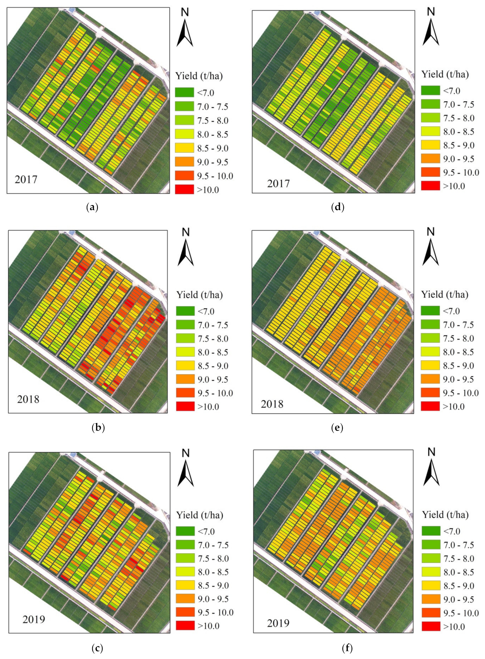
Figure 10.
Yield maps in rice breeding from 2017 to 2019: (a–c) measured yield and (d–f) simulated yield from the optimal RF model.
Figure 10.
Yield maps in rice breeding from 2017 to 2019: (a–c) measured yield and (d–f) simulated yield from the optimal RF model.

Table 1.
Basic information of sowing and transplanting dates across rice cultivars.
| Year | Plots | Cultivars | Sowing Date | Transplanting Date |
|---|---|---|---|---|
| 2017 | 366 | 122 | June 7–10 | July 9 |
| 2018 | 381 | 127 | June 10 | June 29 |
| 2019 | 315 | 105 | June 6 | June 27 |
Table 2.
Summary of VIs or bands derived from UAV images.
| Vegetation Index or Band | Formula | Reference |
|---|---|---|
| R band of UAV image (R) | DN values of R band | -- |
| G band of UAV image (G) | DN values of G band | -- |
| B band of UAV image (B) | DN values of B band | -- |
| Normalized red index (NRI) | R/(R + G + B) | [41] |
| Normalized green index (NGI) | G/(R + G + B) | [41] |
| Normalized blue index (NBI) | B/(R + G + B) | [41] |
| Normalized excess green index (E × G) | (2G − R − B)/(G + R + B) | [42] |
| Normalized excess red index (E × R) | (1.4R − G)/(G + R + B) | [43] |
| Green–red ratio index (G/R) | G/R | [44] |
| Green–blue ratio index (G/B) | G/B | [44] |
| Red–blue ratio index (R/B) | R/B | [44] |
| Green minus red index (GMR) | G − R | [45] |
| Color intensity index (INT) | (R + G + B)/3 | [46] |
| Green and red index (VIgreen) | (G − R)/(G + R) | [47] |
Table 3.
Description of parameters tuned in RF regression models.
| Parameter | Range | Interval | Model | ||
|---|---|---|---|---|---|
| RF (VIs) | RF (Phenology) | RF (Vis + Phenology) | |||
| max_depth | 2–8 | 1 | 2 | 3 | 4 |
| min_samples_split | 2–14 | 2 | 12 | 8 | 12 |
| min_samples_leaf | 2–16 | 2 | 8 | 10 | 4 |
Table 4.
Soil properties of five soil layers at the experiment site.
| Layer (cm) | Clay (%) | Silt (%) | Organic Carbon (%) | Cation Exchange Capacity (cmol kg−1) | Total Nitrogen (%) |
|---|---|---|---|---|---|
| 0–20 | 26.0 | 28.6 | 2.1 | 14.5 | 0.18 |
| 20–40 | 25.1 | 27.1 | 2.1 | 16.9 | 0.20 |
| 40–60 | 23.0 | 25.7 | 1.7 | 17.1 | 0.17 |
| 60–80 | 23.0 | 27.9 | 1.5 | 17.2 | 0.19 |
| 80–100 | 24.5 | 28.0 | 1.6 | 14.6 | 0.16 |
Table 5.
Descriptive statistics of measured yield (t ha−1) and GDL for all cultivars and 21 replicated cultivars across the years.
Table 5.
Descriptive statistics of measured yield (t ha−1) and GDL for all cultivars and 21 replicated cultivars across the years.
| Statistical Indicator | Data Set | Year | Cultivars | Descriptive Statistics | ||||
|---|---|---|---|---|---|---|---|---|
| Minimum | Maximum | Mean | SD | CV (%) | ||||
| Yield | All cultivars | 2017 | 122 | 5.67 | 9.62 | 8.01 | 0.84 | 10.51 |
| 2018 | 127 | 7.61 | 11.01 | 8.99 | 0.60 | 6.7 | ||
| 2019 | 105 | 6.79 | 10.67 | 8.72 | 0.64 | 7.3 | ||
| Replicated cultivars | 2017 | 21 | 7.08 | 9.51 | 8.84 | 0.64 | 7.22 | |
| 2018 | 21 | 7.82 | 9.93 | 8.93 | 0.58 | 6.46 | ||
| 2019 | 21 | 7.70 | 9.74 | 8.82 | 0.55 | 6.28 | ||
| GDL | All cultivars | 2017 | 122 | 123 | 148 | 137 | 5.02 | 3.68 |
| 2018 | 127 | 117 | 130 | 124 | 2.1 | 1.71 | ||
| 2019 | 105 | 117 | 144 | 132 | 4.6 | 3.47 | ||
| Replicated cultivars | 2017 | 21 | 125 | 136 | 129 | 2.59 | 2.01 | |
| 2018 | 21 | 120 | 130 | 125 | 2.72 | 2.17 | ||
| 2019 | 21 | 119 | 134 | 127 | 3.65 | 2.86 | ||
Note: GDL represents growth duration length (d) from sowing to maturity. SD and CV represent standard deviation and variation coefficient, respectively.
Table 6.
Statistics of RF models for yield estimation in calibration (747 plots in 2017 and 2018) and validation (315 plots in 2019) sets.
Table 6.
Statistics of RF models for yield estimation in calibration (747 plots in 2017 and 2018) and validation (315 plots in 2019) sets.
| Model | Calibration Set | Validation Set | ||||
|---|---|---|---|---|---|---|
| R2 | RMSE (t ha−1) | MAE (t ha−1) | R2 | RMSE (t ha−1) | MAE (t ha−1) | |
| RF (VIs) | 0.52 | 0.61 | 0.49 | 0.06 | 0.65 | 0.51 |
| RF (phenology) | 0.62 | 0.54 | 0.43 | 0.46 | 0.51 | 0.39 |
| RF (VIs + phenology) | 0.70 | 0.48 | 0.38 | 0.53 | 0.43 | 0.34 |
Table 7.
Paired-samples t-tests for difference comparisons between the simulated values of the CERES-Rice model and the optimal RF model for 21 cultivars in 2019.
Table 7.
Paired-samples t-tests for difference comparisons between the simulated values of the CERES-Rice model and the optimal RF model for 21 cultivars in 2019.
| Model | Cultivars | Statistical Indicators | Mean Paired Differences (t ha−1) | Significance (p Value) | ||
|---|---|---|---|---|---|---|
| R2 | RMSE (t ha−1) | MAE (t ha−1) | ||||
| RF (VIs + phenology) | 21 | 0.51 | 0.44 | 0.38 | −0.07 | 0.69 |
| CERES-Rice | 21 | 0.80 | 0.48 | 0.42 | ||
Note: The paired-sample t-test was analyzed at the significant level p = 0.05.
Publisher’s Note: MDPI stays neutral with regard to jurisdictional claims in published maps and institutional affiliations. |
© 2021 by the authors. Licensee MDPI, Basel, Switzerland. This article is an open access article distributed under the terms and conditions of the Creative Commons Attribution (CC BY) license (https://creativecommons.org/licenses/by/4.0/).
Share and Cite
MDPI and ACS Style
Ge, H.; Ma, F.; Li, Z.; Du, C. Grain Yield Estimation in Rice Breeding Using Phenological Data and Vegetation Indices Derived from UAV Images. Agronomy 2021, 11, 2439. https://0-doi-org.brum.beds.ac.uk/10.3390/agronomy11122439
AMA Style
Ge H, Ma F, Li Z, Du C. Grain Yield Estimation in Rice Breeding Using Phenological Data and Vegetation Indices Derived from UAV Images. Agronomy. 2021; 11(12):2439. https://0-doi-org.brum.beds.ac.uk/10.3390/agronomy11122439
Chicago/Turabian StyleGe, Haixiao, Fei Ma, Zhenwang Li, and Changwen Du. 2021. "Grain Yield Estimation in Rice Breeding Using Phenological Data and Vegetation Indices Derived from UAV Images" Agronomy 11, no. 12: 2439. https://0-doi-org.brum.beds.ac.uk/10.3390/agronomy11122439
Note that from the first issue of 2016, this journal uses article numbers instead of page numbers. See further details here.