Article

Dynamic Energy Exchange Modelling for a Plastic-Covered Multi-Span Greenhouse Utilizing a Thermal Effluent from Power Plant

1
Department of Rural Systems Engineering, Research Institute for Agriculture and Life Sciences, College of Agriculture and Life Sciences, Seoul National University, Gwanakno 1, Gwanakgu, Seoul 08826, Korea
2
Research Institute for Agriculture and Life Sciences, College of Agriculture and Life Sciences, Seoul National University, Gwanakno 1, Gwanakgu, Seoul 08826, Korea
3
Department of Smart Farm Engineering, College of Industrial Sciences, Kongju National University, 54 Daehak-ro, Yesan-eup, Yesan-gun 32439, Korea
4
Department of Agricultural and Biosystems Engineering, College of Engineering, Mariano Marcos State University, Batac 2906, Philippines
*
Author to whom correspondence should be addressed.
Submission received: 31 May 2021 / Revised: 16 July 2021 / Accepted: 20 July 2021 / Published: 22 July 2021

Abstract

:
To utilize the energy in the thermal effluent, many attempts have been made to use the thermal effluent for agricultural facilities such as greenhouses. As the first step, it is important to estimate the energy loads of the greenhouse for deciding a suitable scale for the heating and cooling. Then, it is available to estimate the energy efficiency of the thermal effluent heat pump system installed in the greenhouse. Therefore, the main objectives of this study were to design and validate an energy model of the experimental greenhouse growing Irwin mangoes and to estimate the annual and maximum energy loads using building energy simulation (BES). Field experiments were conducted in a multi-span plastic-covered greenhouse growing Irwin mangoes to measure the internal environments of the greenhouse and crop characteristics. The energy exchange model of the greenhouse considering crop, cladding, heat pump was developed using BES. The BES model was validated using the data measured at field experiments. The designed model was found to be able to provide satisfactory estimates of the changes of the internal air temperature of the greenhouse (R2 = 0.94 and d = 0.97). The hourly energy loads computed by using the validated model were used to analyse the periodic and maximum energy loads according to the growth stage of the cultivated crops. Finally, the energy costs were compared according to the type of energy source based on the calculated annual energy loads. The average energy cost when using the thermal effluent—heat pump system was found to be 68.21% lower than that when a kerosene boiler was used.

1. Introduction

As South Korea has four distinct seasons, it is difficult to produce crops via field culture throughout the year. Greenhouses can control the growing environment of crops and produce high-quality crops all through the year. Therefore, the greenhouse cultivation in South Korea increased from 23,669 ha in 1990 to 51,226 ha in 2018. To maintain optimum growing environments for the crops, approximately 30% of all greenhouses utilized cooling and heating systems. Among them, approximately 85% of all greenhouse farmers used fossil fuel as an energy source [1]. Additionally, the heating cost of the greenhouse have been a large percentage of the total production cost because of four distinctive seasons in South Korea. Accordingly, farmers have been burdened with production costs such as energy costs.
After the Industrial Revolution, the dependence on fossil fuels increased globally due to the use of petroleum, natural gas, and coal in machines. Moreover, the world population has increased approximately 1.7% per year for the last 50 years [2]. As energy consumption per capita increased from 1.46 ton of oil equivalent (TOE) year−1 in 1981 to 1.86 TOE year−1 in 2017, the energy consumption around the world has also increased from 6582.9 million TOE year−1 to 14,034.9 million TOE year−1. Along with a dramatic rise in energy consumption, global issues such as global warming, climate change, and energy crunch have arisen, which have attracted interest in new energy sources for replacing fossil fuels. Therefore, attempts have been made to utilize water power, wind power, geothermal heat, and other sources. While the country underwent rapid development, the energy consumption in South Korea increased from 38.9 million TOE year−1 in 1981 to 232.7 million TOE year−1 in 2018. In addition, due to high population density and lack of natural resources, South Korea imported 93.7% of the total energy consumption from abroad in 2018 [3]. Thus, the South Korea government established the Energy Act, Energy Use Rationalization Act, Sustainable Development Act, and other acts with the objective of reducing the total energy consumption and improving the energy efficiency. In addition, the Ministry of Agriculture, Food and Rural Affairs provides financial aid to greenhouse farms that use renewable energy to lower the reliance on imported fossil fuels and improve the efficiency of energy usage [4].
In South Korea, more than 80% of the total energy production was from thermal power generation or nuclear power generation. During energy production, thermal and nuclear power plants waste approximately 56% of the total energy input by heating up the engine. The power plants mostly use seawater to cool down the engine and discharge the heated seawater, which was known as thermal effluent. As the thermal effluent absorbed the waste heat of the power plant, it contains a massive amount of thermal energy. Thermal and nuclear power plants around the country discharge approximately 55.2 billion tons of thermal effluent per year. This includes approximately 388,000 GWh of thermal energy, which can be utilized as an energy source. The total amount of thermal energy in the thermal effluent can easily cover the entire heating energy for greenhouses in South Korea and can reduce the energy cost of greenhouses [5]. To use the thermal energy of the thermal effluent for the greenhouse heating and cooling systems, various types of equipment, such as water storage tanks, heat pumps, heat storage tanks, and fan coil units, must be considered. To use energy more efficiently, each component should be properly designed based on the energy loads of the greenhouses. As the amount of available thermal energy in the thermal effluent changes with time, the energy loads of greenhouses should be estimated as functions of a time variable, such as the season or the crop growth stage.
The methods for estimating the building energy loads can be divided into static methods and dynamic methods according to the time factor. Energy loads are calculated while assuming that the internal and external environments are in a steady state in a static method. In the case of greenhouses, regardless of the type, maximum energy loads can be calculated based on the ambient air temperature and the solar radiation on the warmest and coldest days. Periodic energy loads can be calculated from the accumulated difference between the optimum growth temperature of cultivation crops and the external air temperature [6,7]. The static methods have the disadvantage of not considering the thermal storage of structure by solar radiation and internal heat sources [8]. This can be problematic, especially in greenhouses, as the cladding is much thinner than in general buildings and, hence, is much more sensitive to changes in weather conditions. In addition, the energy exchange between crops in the greenhouse and the ambient air change drastically over time [9]. Therefore, when calculating energy loads of greenhouses via a static method, the calculated energy loads were different from the actual energy loads. In contrast, a dynamic method considers the actual energy flow under an unsteady state. A dynamic method is a method for calculating the energy balance of a structure over time via numerical analysis. With a dynamic method, energy loads are calculated by simulating the energy exchange using real-time weather data. The energy balance equation for a specified time was analysed, and the amounts of energy exchange and thermal storage of each component were passed to the next time step. In architecture, a building energy simulation (BES) technique was typically used as a dynamic method for calculating energy loads with high accuracy and performance. Recently, this technique has also been used in agriculture to simulate energy exchange in greenhouses dynamically and to validate the dynamic energy exchange model of a greenhouse [10,11,12,13,14,15]. Therefore, it is necessary to use a dynamic method to simulate the energy exchange in greenhouses more precisely by considering the internal and external environmental changes of the greenhouse.
The objective of this study was to design and validate an energy model of the experimental greenhouse growing Irwin mangoes and to estimate the annual and maximum energy loads using building energy simulation (BES). The experimental greenhouse was constructed near the power plant to enhance the energy efficiency of the heating and cooling system by utilizing a thermal effluent. The system for using thermal effluent was installed at the experimental greenhouse without quantitative analysis and design. The dynamic energy exchange model of the greenhouse was developed considering the greenhouse structure, the operational conditions of the thermal screens and vent openings, an energy exchange of the crops, and the thermal effluent–heat pump. The periodic and maximum energy loads were calculated using the developed energy exchange model. Then, the impact of the energy exchange by crops was analysed when calculating the energy loads of the greenhouse. Additionally, the energy costs according to the utilization of the thermal effluent were analysed.

2. Materials and Methods
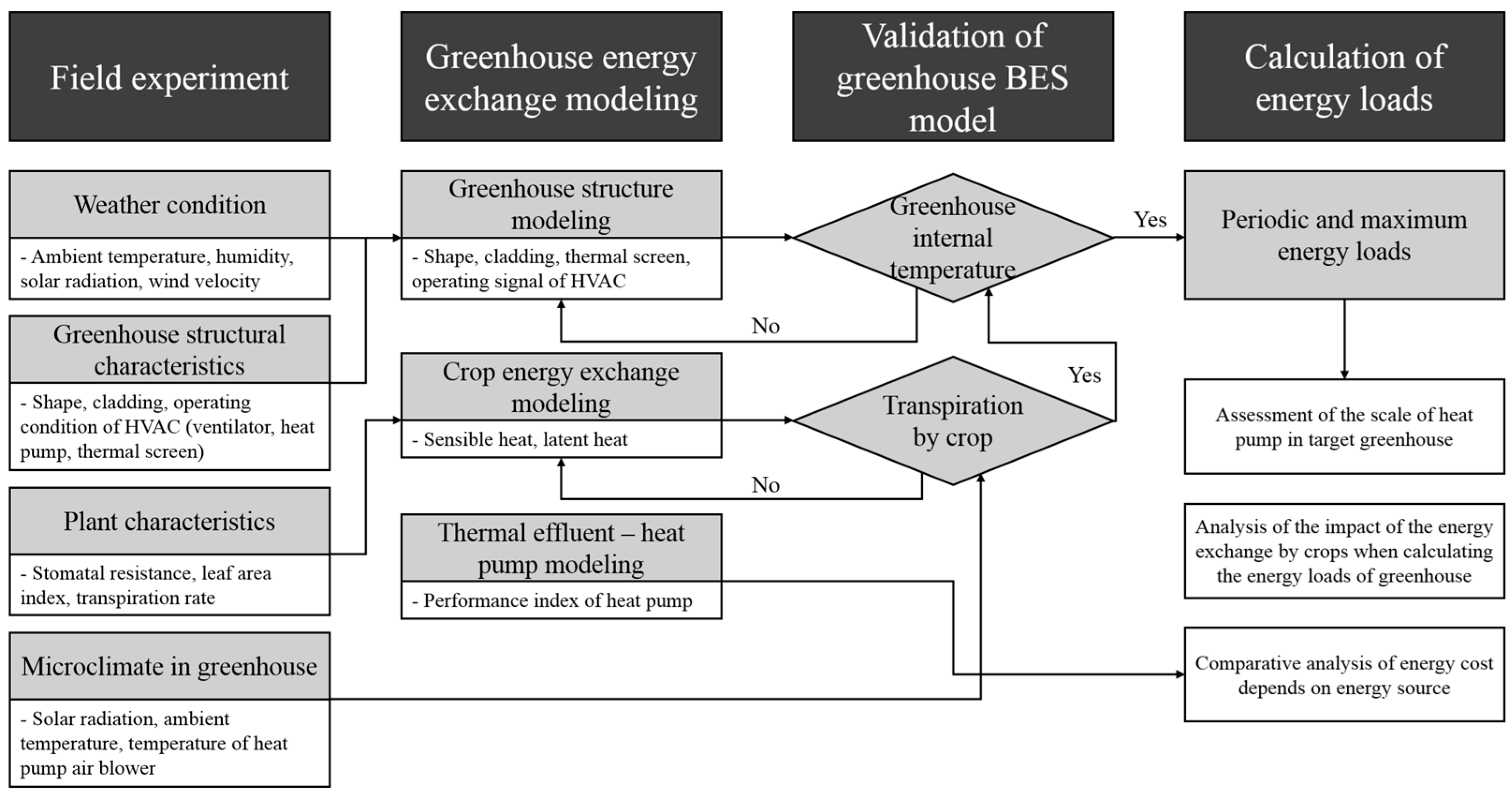
2.1. Research Flow

A flowchart for the design of a dynamic energy exchange model of the greenhouse and the calculation of the energy loads is presented in Figure 1. The weather data of the target area were analysed and field experiments were conducted to design an energy model of the greenhouse growing Irwin mangoes. Greenhouse structural characteristics, such as the shape, cladding, and heating and cooling system, were investigated for the design of the greenhouse structure model, and crop characteristics, such as the stomatal resistance and leaf area index (LAI), were measured for the design of the crop energy exchange model. The internal and external environments of the greenhouse such as the solar radiation, the air temperature, and relative humidity were also measured to validate the energy model. The experimentally measured transpiration rate of the crops and the ambient air temperature inside the greenhouse were used to validate the energy exchange model of the crops and the entire greenhouse, respectively. Based on the validated greenhouse energy exchange model, the periodic energy loads which refer to the total energy load at certain periods were calculated according to the crop growth stage. Additionally, the peak energy loads referred to as maximum energy at certain periods were also calculated according to the crop growth stage. Energy loads were calculated using the actual weather data of 10 years (1 June 2009–31 May 2019) for accurate simulations [16]. Energy loads were used to analyse the trends according to the weather conditions and to derive the average energy loads. The hourly energy load data were used to calculate periodic energy loads and to analyse the energy cost and maximum energy loads to decide the proper scale of a heat pump in the greenhouse. The effects of crop energy exchange on energy loads of greenhouses were analysed by comparing the cooling and heating loads with versus without consideration of the crops. Finally, a comparative analysis of the energy costs was conducted according to an energy source as an essential prerequisite for the utilization of the thermal energy of the thermal effluent.

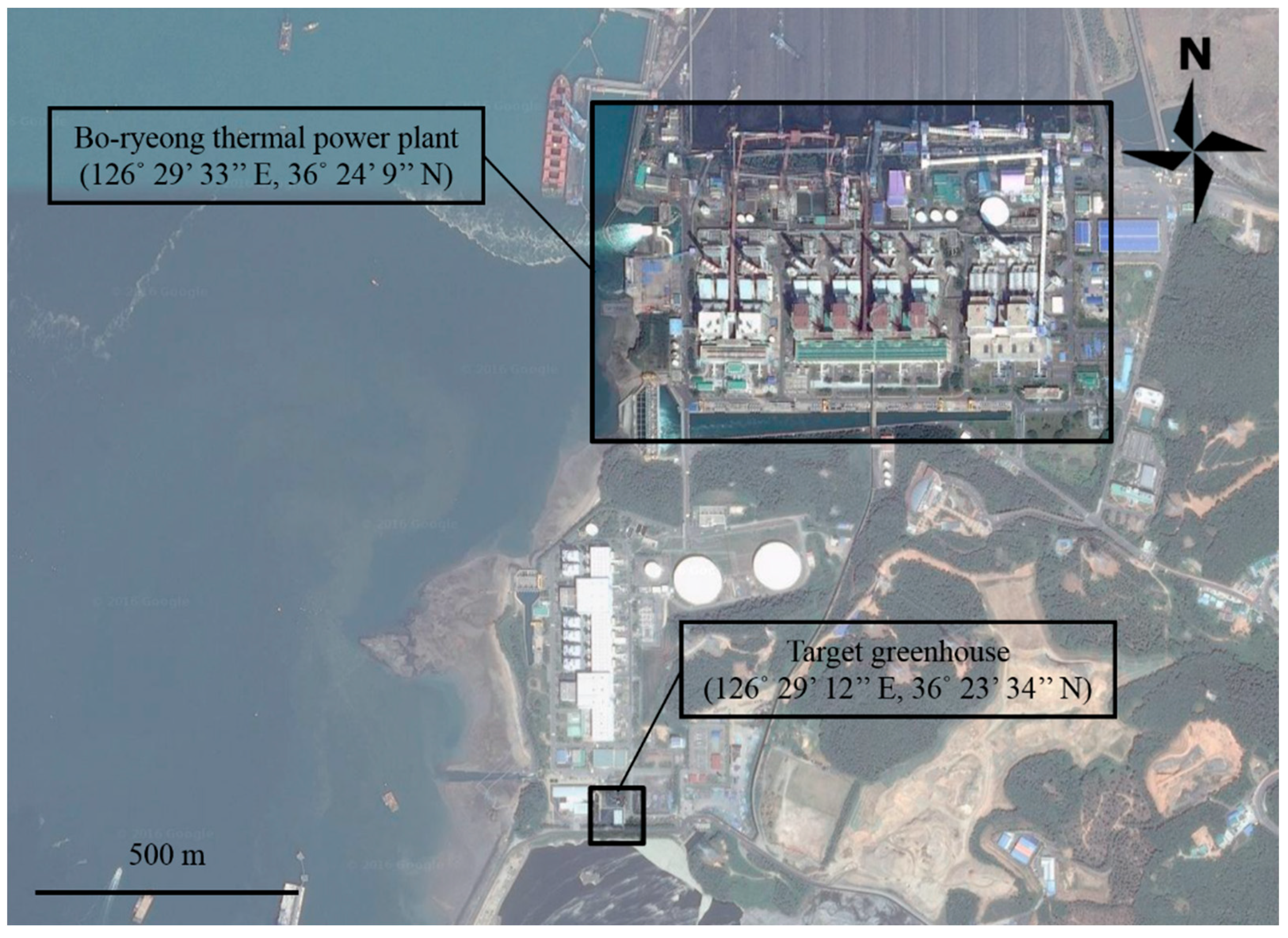
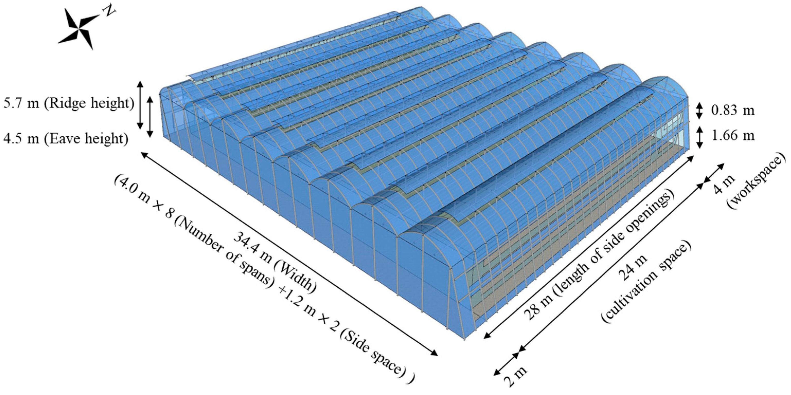
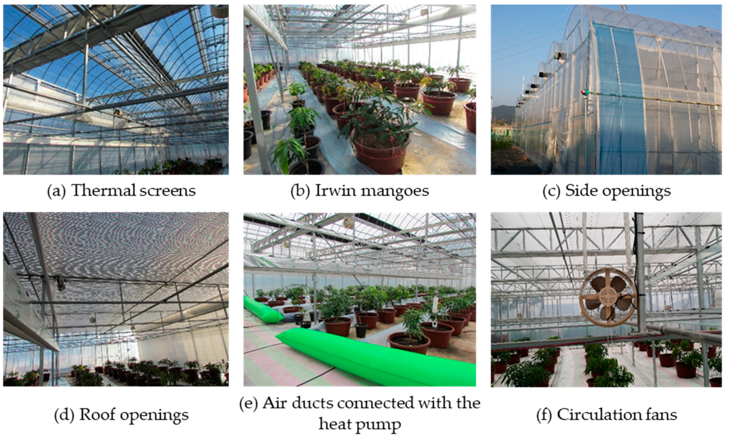
2.2. Experimental Greenhouse

The experimental greenhouse was located on the west coast of South Korea in Jugyo-myeon, Bo-ryeong City, Chungcheongnam-do Province (126°29′ E, 36°23′ N), which was 1 km south of the Bo-ryeong thermal power plant (Figure 2). The experimental greenhouse was constructed to enhance the energy efficiency of the heating and cooling system by utilizing a thermal effluent. The experimental greenhouse was an eight-span 1-2-W-type greenhouse, as illustrated in Figure 3. Figure 4 shows thermal screens, crops, vent openings, air ducts that were connected with the heat pump, and circulation fans in the greenhouse. The experimental greenhouse had a width of 34.4 m, a length of 30.0 m, an eave height of 4.5 m, and a ridge height of 5.7 m. The covering of the greenhouse was made of a 0.15 mm thick polyolefin film. The greenhouse was divided into a cultivation space (768 m2 floor area) for cultivating Irwin mangoes and a workspace for controlling the mechanical system (128 m2 floor area) (Figure 3). The sides of the experimental greenhouse were covered with double-layer polyolefin film for additional insulation. Thermal screens were installed at the sidewall and ceiling height to decrease conduction heat loss that were caused by outdoor versus indoor air temperature differences at the cladding. After sunset, the thermal screen at the sidewall was drawn vertically, and the thermal screen at the ceiling was installed horizontally at a height of 3.8 m from the floor. The greenhouse was occupied with 100 potted Irwin mango fruit trees. In the experimental greenhouse, the mango trees were pruned to a height of approximately 1.5 m, and the branches were pulled into a globular shape to equalize the light-interception. Therefore, the mango trees in the greenhouse were fixed in shape and size during the experimental periods.
The thermal effluent from the Bo-ryeong power plant was used as a heat source to operate the heat pump. The facility discharges thermal effluent at a rate of approximately 3 billion tons per year. The thermal effluent was stored initially in a water storage tank and utilized on the farm and in the greenhouse. The internal environment of the greenhouse was controlled using natural ventilation with side and roof vents and was heated or cooled using three heat pumps (ADF-SLX12WHB, A-San Inc., Gimpo, South Korea). These actuators were controlled automatically based on the internal air temperature and the external solar radiation. The performance of the heat pump was 43,276 W in maximum cooling capacity and 36,786 W in maximum heating capacity. To supply heat energy uniformly, air ducts and circulation fans were installed in the greenhouse. The 16 circulation fans (SGA-300P, Shinan Green Tech Co., Sun-cheon, South Korea) have a capacity of 35 m3 min−1 per unit and were installed at a height of 2.5 m above the ground floor.

2.3. Building Energy Simulation (BES)

Estimation of the energy loads is important for designing the greenhouse and enhancing the efficiency of energy usage. The TRNSYS program (Version 18, Solar Energy Laboratory, University of Wisconsin-Madison, Madison, WI, USA), among several BES programs, was used to model the energy exchange of the greenhouse. TRNSYS program has the advantage of a module-based program, which consists of the main program and several sub-modules to analyse energy flow of each component. TRNSYS also has the advantage of availability and compatibility on an enormous energy system because of a number of sub-modules which can compose various systems such as heat pumps, energy exchange of crop, ventilation. The target building component, which was the experimental greenhouse in this study, consists of several zones. The energy balance equation (Equation (1)) was calculated by zone to simulate the thermal behavior for each zone. It was assumed that the energy exchange by the condensation on the cladding of the greenhouse was relatively small in this study because of the double-layer polyolefin film and thermal screen for reducing heat loss.
Q i = Q s u r f + Q i n f + Q v e n t + Q i s h c c i + Q s o l a r + Q g , c + Q c p l g
where, Q i is the total heat gain of zone I (kJ), Q s u r f is the convective heat gain or loss from surfaces (kJ h−1), Q i n f is the heat gain or loss by infiltration (kJ h−1), Q v e n t is the heat gain or loss by ventilation (kJ h−1), Q i s h c c i is the absorbed solar radiation on all internal shading devices of zone and directly transferred as a convective gain to the internal air (kJ h−1), Q s o l a r is the fraction of solar radiation entering a zone (kJ h−1), Q g , c is the internal convective gains (kJ h−1), and Q c p l g is the heat gain or loss due to connective air flow from adjacent zone (kJ h−1).

2.4. Experimental Procedure

2.4.1. Field Experiments

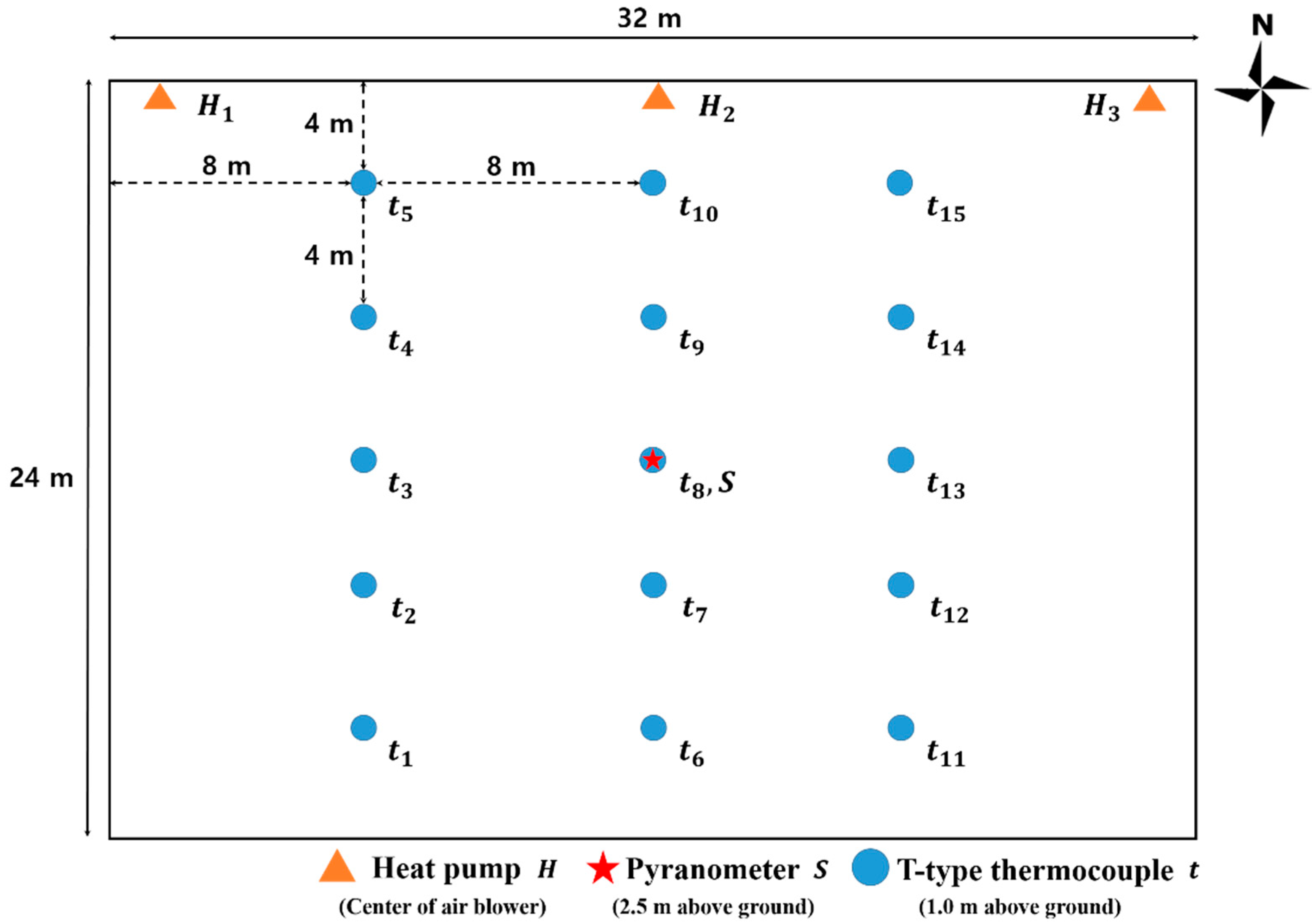
Measurement of the Internal Environment in the Greenhouse

The internal environments of the experimental greenhouse were monitored to design and validate the energy exchange model of the greenhouse (Figure 5). A field experiment was conducted from 28 May to 1 June 2016. To measure the radiation transmissivity of the greenhouse cladding, a pyranometer (SP-110; Apogee Inst., Logan, UT, USA) was installed on the center of the top frame, which was 2.5 m above the bottom floor. The internal air temperature of the greenhouse was measured by a thermocouple (T-type; Ondo114 Co., Seoul, South Korea), which was installed 1.0 m above the ground. Fifteen thermocouples were installed for calculating the average air temperature and three thermocouples were installed at the center of the air blower of each heat pump for monitoring the operating time of the heat pump during the experimental period. The installed sensors were connected to a data logger (GL 820; Graphtech Corp., Irvine, CA, USA), and the data were saved at five-second intervals.

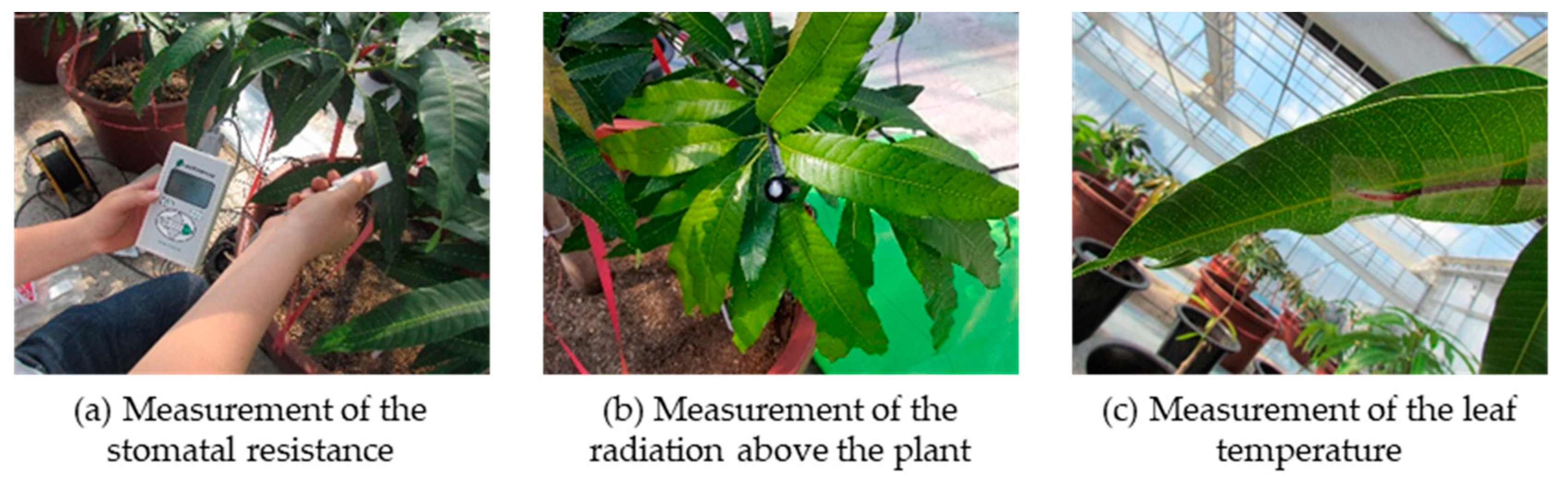
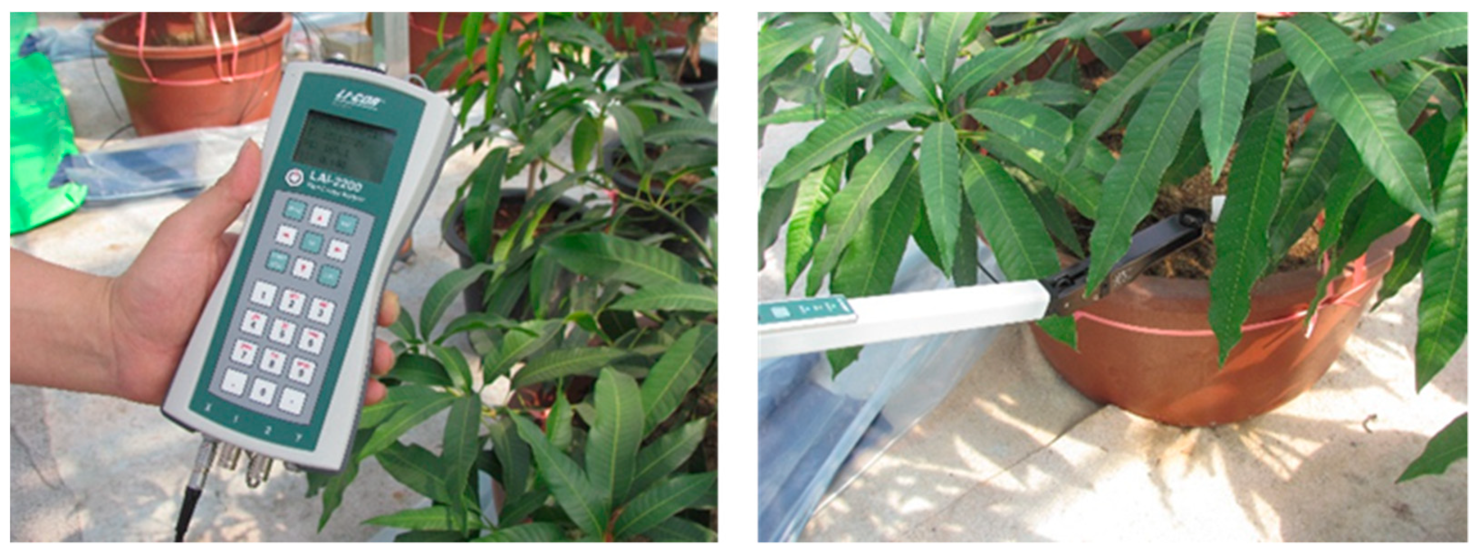
Measurement of the Stomatal Resistance and the Leaf Area Index of Crops

As the Irwin mango is a perennial plant, it was assumed that the stomatal resistance was constant with growth in this study. The stomatal resistances at the ventral and dorsal sides of the top, middle, and bottom leaves of the crops in the experimental greenhouse were measured at the 17–18 May 2016 using a leaf porometer (SC-1; Decagon devices, Pullman, WA, USA) (Figure 6). A leaf porometer is a sensor that measures the vapor conductivity per unit area and calculates the stomatal resistance as the reciprocal of the vapor conductivity. The radiation above the plants was measured by a pyranometer, and the surface temperature of the leaf was measured by installing a thermocouple on the ventral side of the leaf. A regression equation for estimating the stomatal resistance from the measured radiation and the leaf temperature was derived and applied as a parameter for an energy exchange model of the crops.
LAI is the ratio of the whole leaf area to the ground area that is covered by plants, which represents the leaf distribution and density. LAIs of 100 crops were measured at 17 February 2016 and 10 April 2016 using a plant canopy analyser (LAI-2200; LI-COR Inc., Lincoln, NE, USA) (Figure 7). LAIs were used to calculate the average LAI of the crops in the greenhouse. Based on the Beer–Lambert law, LAI was calculated from the radiation above and under the canopy, which was measured by a plant canopy analyser. The average LAI of 100 crops was applied in the design of the energy exchange model of the crops.

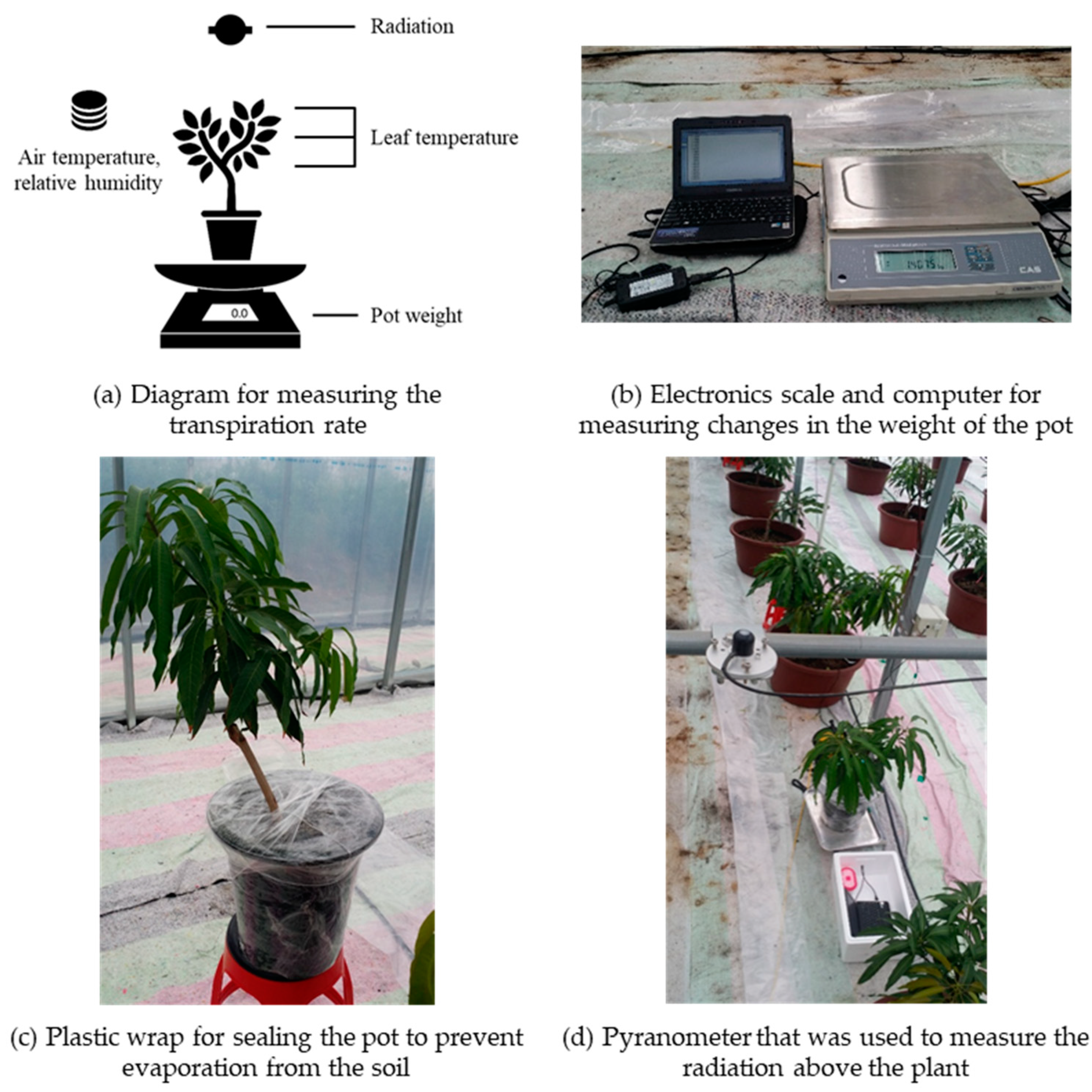
Measurement of Transpiration by Crops

Transpiration is directly related to the latent heat and, therefore, was used as data for validation (Equation (2)). To validate the energy exchange model of the crops, the calculated transpiration rates of the crops were compared with the measured transpiration rates. The ambient air temperature, relative humidity, surface temperature of the leaf, stomatal resistance, and LAI were measured from 28 May to 1 June 2016 and used to calculate the transpiration rate. Figure 8 show the diagram and the arrangement of the experimental equipment for measuring the transpiration rate. The crops were three-year-old Irwin mangoes that were cultivated in a 44.5 cm diameter pot. The pot was placed on an electronic scale (CBX32KH; CAS Corp., Seoul, South Korea) to measure the change in the weight of the pot over time. The weight of the pot was recorded at five-minute intervals, excluding the watering periods. To exclude water evaporation from the soil and to measure only transpiration from the plant, the soil part of the pot was sealed with plastic wrap. A pyranometer was installed on the centre of the top frame and was used to measure the radiation, and 3 thermocouples were installed on the dorsal side of the leaf (top, middle, and bottom) and were used to measure the surface temperature of the leaf. Three HOBO data loggers (UX100-003; Onset Corp., Bourne, MA, USA) were also installed near the plant to measure the ambient air temperature and the relative humidity.
E = L E λ
where E is the transpiration per area (kg s−1 m−2), LE is the latent heat flux (W m−2), and λ is the latent heat of vaporization of water (J kg−1).

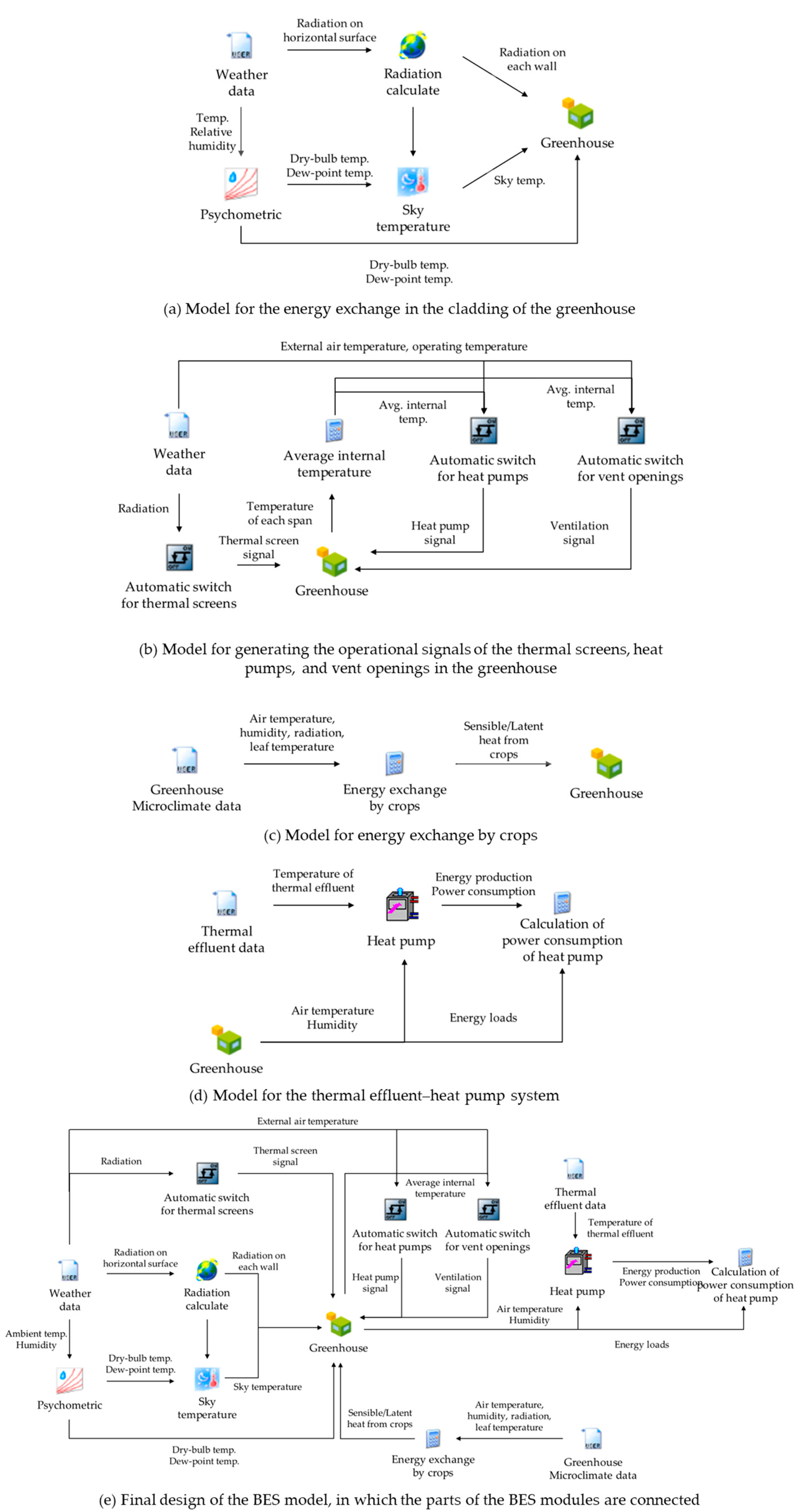
2.4.2. Design of the Energy Exchange Model of the Greenhouse

A dynamic energy exchange model of the greenhouse was designed by adapting four models: A model of the greenhouse structure, a model for generating the operational signals of the thermal screens, heat pumps, and vent openings, an energy exchange model of the crops, and a model of the thermal effluent–heat pump. Several modules in TRNSYS, such as the data reader module for reading weather data as input data and the psychrometric module for calculating the properties of moist air, were used for each part of the model (Table 1).
As the energy exchange via radiation and conduction at the cladding depends on the shape and materials of the greenhouse, it was important to model the greenhouse cladding precisely. The multi-zone module was used to design the structure of the greenhouse according to geometric information on the experimental greenhouse (Figure 3). The structure data and cladding data for the greenhouse model were applied to the multi-zone module using the TRNSYS plugged-in SketchUp program (ver. 8, Google, Mountain View, CA, USA) and the WINDOW program (ver. 7.4, LBNL, Berkeley, CA, USA), respectively. As the multi-zone module cannot create the internal wall in a single zone, the crop growth space was divided horizontally to set the thermal screen in the greenhouse. The physical properties of the 0.15 mm polyolefin film that was used for the cladding of the greenhouse were specified as follows: thermal conductivity of 0.330 W m−1 K−1, solar transmittance of 0.797, solar reflectance of 0.106, visible transmittance of 0.935, visible reflectance of 0.106, and infrared emittance of 0.840. The physical properties of the materials that were used for the frame and floor of the greenhouse were as listed in Table 2. To set the thermal screen, each span was divided into three zones; therefore, there were twenty four zones for the crop growth space. A virtual wall was set up between each span to simulate thermal exchange via convection and between the upper sides of the cultivation space to configure the thermal screen on the working schedule.
The data reader, radiation processor, psychometric, sky temperature calculator and multi-zone module were used to simulate the energy exchange at the cladding in TRNSYS. The solar radiation on each wall, the dew-point temperature, and the sky temperature were calculated at each module using weather data. These calculated data were linked to the multi-zone module for the simulation of the energy exchange via conduction and radiation (Figure 9a).
Inside the experimental greenhouse, the heat pumps, thermal screens and vent openings were operated according to the internal environments. The operating condition for all equipment was measured by a field experiment. The operating conditions were used as a boundary condition into the greenhouse BES model. Switch modules were used to design the thermal screens, heat pumps and vent openings in the greenhouse (Figure 9b). The internal air temperature, the amount of external solar radiation, and the external air temperature were used as input data to generate the operating signal of each equipment. The operating signal can take a value of 0 or 1, and if the value was 1, the equipment operated. The operating conditions of each equipment were determined via Equations (3)–(5), and the operating temperature was established based on the optimum temperature of Irwin mango crops according to the growth period.
T S S I G N = { 1 ( R G = 0 ) 0 ( R G > 0 )
H E A T S I G N = { 1 ( T i n < H E A T T E M P ) 0 ( T i n H E A T T E M P ) C O O L S I G N = { 1 ( T i n > C O O L T E M P ) 0 ( T i n C O O L T E M P )
V E N T S I G N = { 1 ( T i n > V E N T T E M P   a n d   T i n > T o u t ) 0 ( T i n V E N T T E M P )
where T S S I G N is the thermal screen signal, H E A T S I G N is the heating signal, H E A T T E M P is the set temperature of heating,   C O O L S I G N is the cooling signal, C O O L T E M P is the set temperature of cooling, V E N T S I G N is the ventilation signal, V E N T T E M P is the set temperature of ventilation, T i n is the internal air temperature (°C), and T o u t is the external air temperature (°C).
In this study, the sensible and latent heat of crops were used to simulate the energy exchange of crops. The sensible and latent heat of crops were calculated via Equations (6) and (7). The BES modules for the energy exchange of crops are illustrated in Figure 9c. The environmental conditions and characteristics of the crops were used to model the energy exchange model of the crops. The external resistance of the crops ( r e ) was determined in real time based on Equation (8). The characteristic leaf dimension ( l ) was measured for three crops to represent each growth stage of the Irwin mangoes in the greenhouse, and the average value was calculated as 9.99 cm. As the average measured air velocity in the greenhouse was less than 0.1 m s−1, the wind speed ( u ) was set to 0.1 m s−1, which is identical to the value that was used by Stanghellini [17]. The regression model that was derived from the data from the field experiments was used to calculate the stomatal resistance ( r s ). The measured average LAI of the cultivated crops of 1.78 was used as a constant under the assumption that the crops were pruned during the experimental period. The thermal energy that was stored in the plants ( G ) was highly variable according to the radiation. In this study, the thermal energy that was stored in the plants was calculated as 15% of the net radiation flux [18,19].
H = L A I ρ a c p r e ( T L T a )
L E = δ δ + γ * ( R G G ) + δ δ + γ * L A I ρ a λ ( e a * e a ) ÷ r e ( γ * = γ ( 1 + r s r e ) )
r e = 1174 l 0.5 ( l | T L T a | + 207 u 2 ) 0.25
where H is the sensible heat of the crop (W m−2), L E is the latent heat of the crop (W m−2), ρ a is the density of air (kg m−3), c p is the specific heat of air at constant pressure (J kg−1 K−1), T L is the temperature at the surface of the leaf (K), T a is the ambient air temperature (K), r e is the external resistance of the surface of the leaf to sensible heat transfer (s m−1), δ is the slope of the saturation vapor pressure–temperature curve (Pa K−1), γ is the thermodynamic psychometric constant (Pa K−1), r s is the stomatal resistance (s m−1), R G is the solar radiation (W m−2), G is the thermal energy that is stored in the crops (W m−2), L A I is the leaf area index (dimensionless), e a * is the saturation vapour pressure at the air temperature (Pa), e a is the vapour pressure of the air (Pa), l is the characteristic leaf dimension (m), and u is the wind speed (m s−1).
When calculating the energy loads of the greenhouse using historical weather data, a limitation was encountered in simulating the energy exchange of the crop, which was due the absence of real-time environmental data inside the greenhouse. Therefore, the ratio of the sensible and latent heats to the external radiation was used to design the energy exchange model of the greenhouse based on research by [10]. The ratio of the sensible and latent heats from crops to the external radiation was derived from the validated energy exchange model of the crop in this study.
The thermal effluent–heat pump system was modelled based on performance data of the heat pump. Real-time thermal effluent data were used to calculate the rated cooling and heating capacities and the power consumption. The greenhouse internal air temperature and humidity level were considered simultaneously in the calculation of the actual energy production and power consumption levels. The actual calculated energy production and power consumption levels were compared with the energy loads of the experimental greenhouse to simulate the energy consumption of the experimental greenhouse. The BES modules for the thermal effluent–heat pump system are illustrated in Figure 9d. The rated air flow and water flow were set to 2405 and 2.11 l s−1, respectively, and the cooling capacity, heating capacity, and power consumption were set for several inlet water temperatures. The cooling and heating performance data at inlet water temperatures of 1, 5, 10, 15, 20, 25, and 30 °C that were provided by the company were used (Table 3). The performance correction data were additionally applied to consider changes in the performance and the power consumption of the heat pump that were due to the changes in the greenhouse internal air temperature and humidity.
The dynamic energy exchange model of the experimental greenhouse was designed based on the BES technique, which includes the BES models for the greenhouse structure, generating the operational signals, the energy exchange model of crops, and the thermal effluent heat pump system (Figure 9e). Each part was connected to the greenhouse to simultaneously simulate the energy flow. The simulations of the energy exchange model were conducted at 1 min intervals.

2.4.3. Accuracy Evaluation Method for the BES Model

The internal air temperature computed by the designed BES model was compared with internal air temperature measured at the field experiment to evaluate the accuracy of the greenhouse BES model. The simulated transpiration rate was also compared with the measured transpiration rate to evaluate the energy exchange model of the crop. The measured crop characteristics and environmental conditions, such as the LAI, ambient air temperature, humidity, and radiation above the plants, were used to simulate the transpiration rate.
In this study, the coefficient of determination (R2) was used to analyse the tendency. The index of agreement ( d ) was used to assess the error between the simulated data and the measured data [20]. R2 is a coefficient that only indicates the tendency between two groups of data and not the direction or errors. R2 can take a value that is between ‘0’ and ‘1’. The more similar the tendencies of two groups of data are, the closer R2 is to 1 (Equation (9)). The index of agreement can standardize the measure of the degree of the model prediction error, which can take a value between ‘0’ and ‘1’. The closer the index is to 1, the more closely the simulated data correspond to the measured data (Equation (10)).
R 2 = ( i = 1 n ( Y i o b s Y o b s ¯ ) ( Y i s i Y s i ¯ ) i = 1 n ( Y i o b s Y o b s ¯ ) i = 1 n ( Y i s i Y s i ¯ ) ) 2
d = 1 i = 1 n ( Y i o b s Y i s i ) 2 i = 1 n ( | Y i s i Y o b s ¯ | + | Y i o b s Y o b s ¯ | ) 2
where Y i o b s is the i-th measured value, Y o b s ¯ is the average of the measured values, Y i s i is the i-th simulation value, and Y s i ¯ is the average of the simulation values. S T D E V o b s is the standard deviation of the measured values.

2.4.4. Analysis of the Greenhouse Energy Loads

The experimental greenhouse maintains the growing environment in a suitable range of air temperatures for growing the crops. However, to bear fruit, the crops must undergo several growing stages, which have a diverse range of growing temperatures. The air temperatures for heating, cooling and ventilation were set based on the optimum growing temperature for each growth stage (Table 4). Weather data from 2009 to 2019 collected at the Seo-san weather station of the Korean Meteorological Administration (KMA), which is the nearest weather station from the experimental greenhouse, were used to calculate the energy load of the greenhouse. Weather data such as the air temperature, the relative humidity, the wind environment, and the solar radiation were observed at intervals of 1 h. The periodic and maximum energy loads were calculated by summarizing and comparing the hourly energy loads for each year. Periodic energy loads were used to analyse the energy consumptions of the experimental greenhouse according to the growth stages. Maximum energy loads were used to assess the capacities of heating and cooling systems installed at the experimental greenhouse and suggest the proper capacities of cooling and heating systems. Based on the growth periods, the analysis period was from May 30 to June 1 for each year. As the Bo-ryeong thermal power plant only provided five years of discharge flow data, the temperature of the thermal effluent and the daily oil price for the five-year period (2010 to 2014) were used to compare the energy cost, which depends on the energy source.

3. Results and Discussion

3.1. Result of the Field Experiment

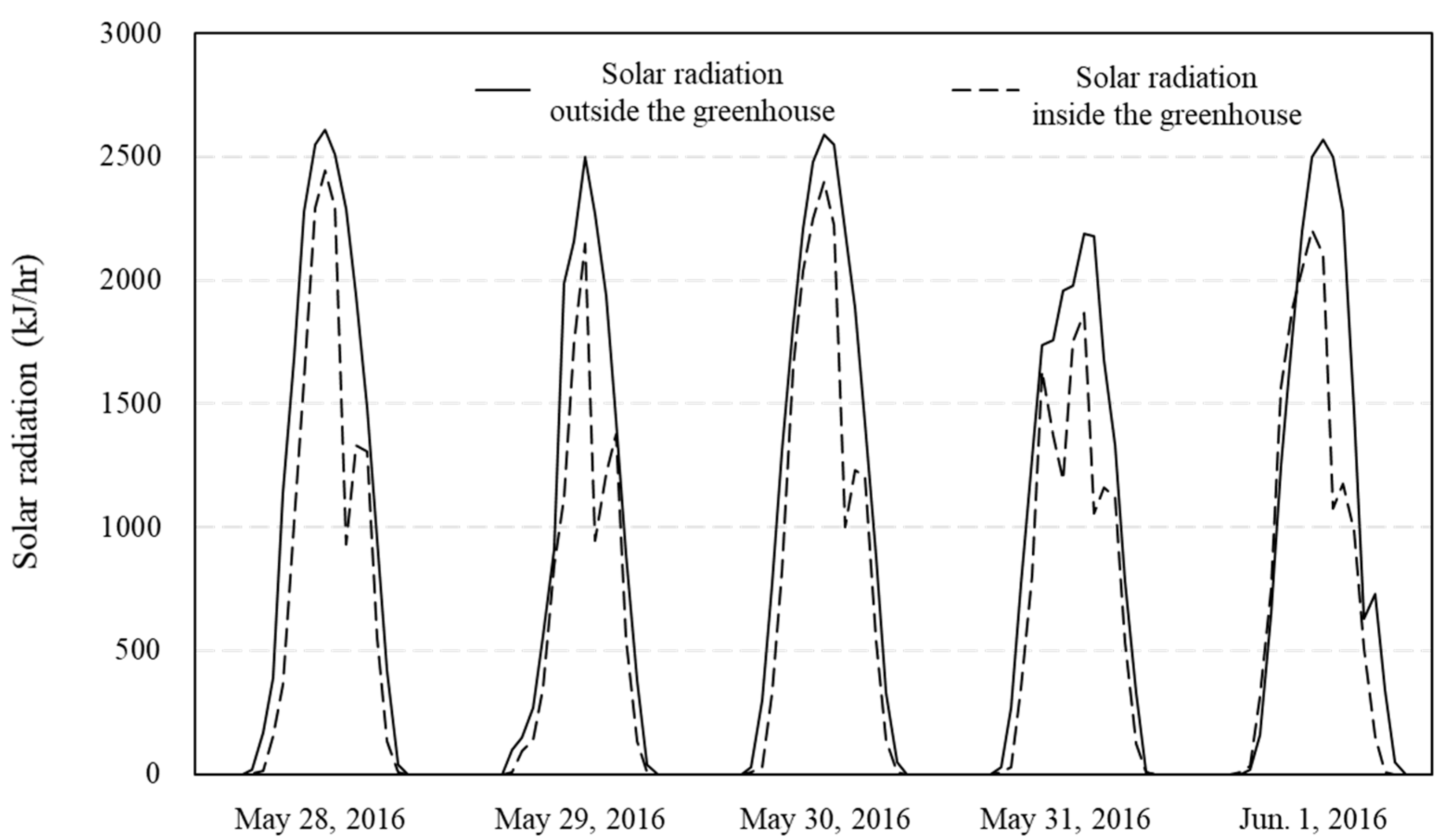
3.1.1. Analysis of the Internal Environmental Data

The internal air temperatures by location and time were analysed according to day (8:00 AM to 8:00 PM) and night (8:00 PM to 8:00 AM) (Table 5). The average air temperature of the entire period was 29.9 °C, and the standard deviation of each location was 0.57 °C, which was low. The average air temperatures and standard deviations for each location were 33.6 and 0.92 °C during day, and 25.4 and 0.30 °C during night, respectively. The standard deviation of each location at night was lower than that during the day because air ducts and circulation fans were installed to ensure that the thermal environment of the crop growth room remains uniform.
Figure 10 shows a graph of the average air temperature at the centres of three heat pump air blowers and the average internal air temperatures of the greenhouse. According to the graph, the set temperatures of the heat pump on 29–31 May were 25 °C, and the air temperature of an air blast was approximately 42 °C when the heat pump was operated. The air temperatures were changed by the operation of the heat pumps. The heat pump did not operate on 28 May because of a mechanical defect, and the set temperature of the heat pump was increased by approximately 2–3 °C on 1 June.
Figure 11 is a graph comparing the internal and external solar radiation of the experimental greenhouse. The trend of the internal solar radiation of the greenhouse usually followed that of the external radiation; however, the internal solar radiation decreased at approximately 2:00 PM every day due to shade from a folded thermal screen. The average radiation transmissivity of the cladding, except for the data at approximately 2:00 PM, was analysed and found to be 83%.

3.1.2. Stomatal Resistance and the Leaf Area Index of the Crops

The field experiment for measuring the stomatal resistance of the crops in the greenhouse was conducted. The stomatal resistances and the leaf temperatures at the ventral and dorsal sides of the top, middle, and bottom leaves were measured. The average stomatal resistances on the two sides of the top, middle, and bottom leaves were analysed, and the average value was found to differ according to the side of the leaf. As the Irwin mango is a perennial plant, the stomata are distributed on the ventral side of the leaf and are scarce on the dorsal leaf. For this reason, there were significantly fewer stomata on the dorsal side of the leaf than on the ventral side. The average stomatal resistance on the dorsal side (top leaf: 2023 s m−1, middle leaf: 1820 s m−1, and bottom leaf: 1906 s m−1) was analysed and found to be much higher than the average stomatal resistance on the ventral side (top leaf: 850 s m−1, middle leaf: 168 s m−1, and bottom leaf: 264 s m−1).
A non-linear regression equation for calculating the stomatal resistance from the radiation and the leaf temperature was derived and used as a parameter for the energy exchange model of the crops (Equation (11)). The derived equation was found to simulate the actual stomatal resistance precisely ( R 2 = 0.854 and d = 0.917 ).
r s = 98 [ 1 + { e x p ( 0.011 ( R G 29.836 ) ) } 1 ] [ 1 + { 0.172 e x p ( 0.127 ( T L 36.5 ) ) } ]
To calculate the average LAI of the Irwin mango in the greenhouse, a plant canopy analyser was used to measure the LAIs of 100 Irwin mango pots. As the average LAI of 100 crops was 1.78, the average value of 1.78 was used in the design of the energy exchange model of the crops.

3.2. Design of the Energy Exchange Model

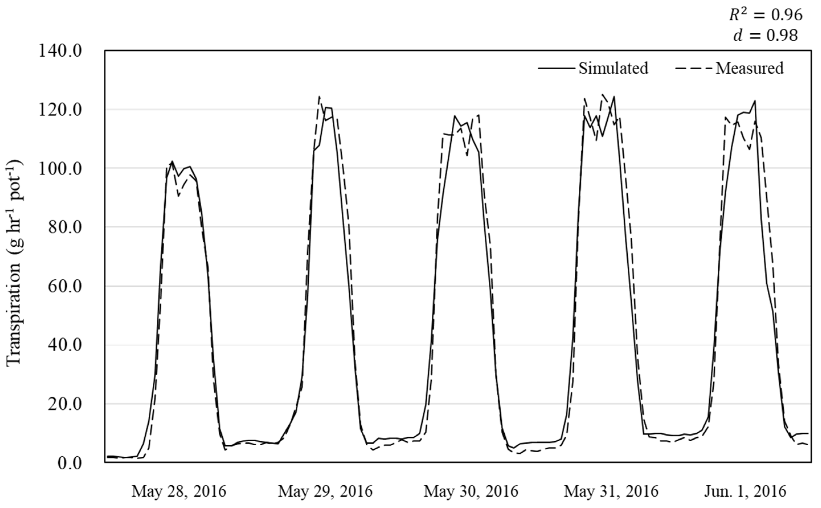
3.2.1. Validation of Transpiration of Crops

To measure the transpiration rate of the crops, the weight of the pot in each case was recorded at five-minute intervals. The results of measuring the transpiration are shown in Figure 12. During the daytime, the crops transpired actively, whereas during the night-time (8:00 PM to 5:00 AM), the average measured transpiration rate was 0.535 g crop−1. However, on the night of 28 May, the average transpiration rate was 0.154 g crop−1, which was 70% lower than those during all night-time periods of the experimental period. This result stemmed from the water content of the plants, which rose after the May 28, as irrigation provided half of a litre of water typically at 9:00 AM, while one litre of water was provided by irrigation every evening at 9:00 PM during the experimental period. For the same reason, the average transpiration rate during the daytime (9:00 AM to 6:00 PM) on 28 May (7.212 g crop−1) was found to be 15% lower than all daytime amounts during the experimental period (8.427 g crop−1).
To validate the energy exchange model of the crops, the transpiration rate that was measured by the field experiment was compared with the simulated data. Measured data at five-minute intervals and simulated data at one-minute intervals were compared (Figure 12). The designed energy exchange model of the crops was validated as providing a satisfactory estimate of the change in the transpiration rate throughout the experimental period ( R 2 = 0.96, d = 0.98). Considering the error on 28 May, with a dataset of four days that does not include the first day, the energy exchange model of the crops that was designed in this study was found to reflect the actual latent heat from the crops accurately.

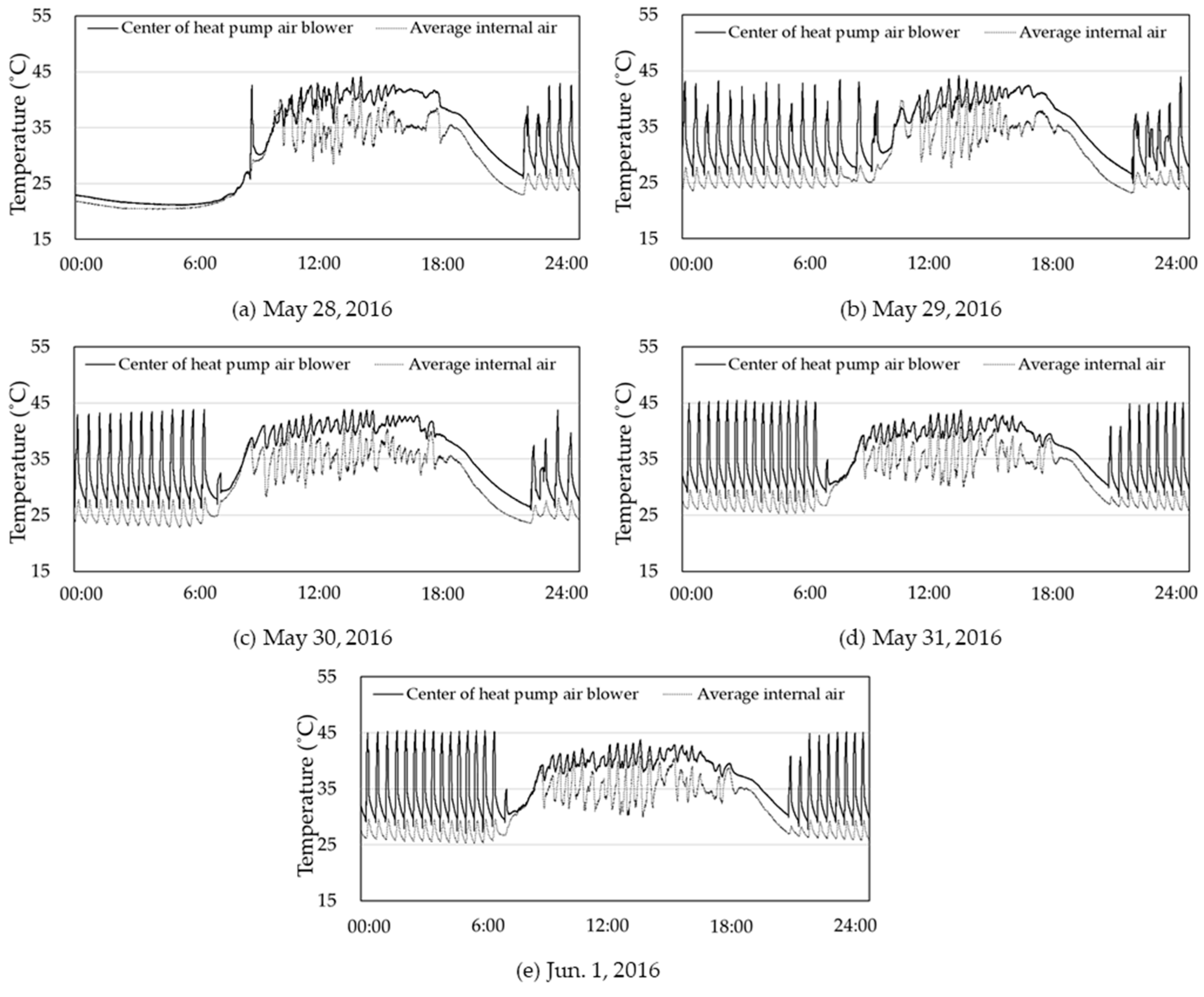
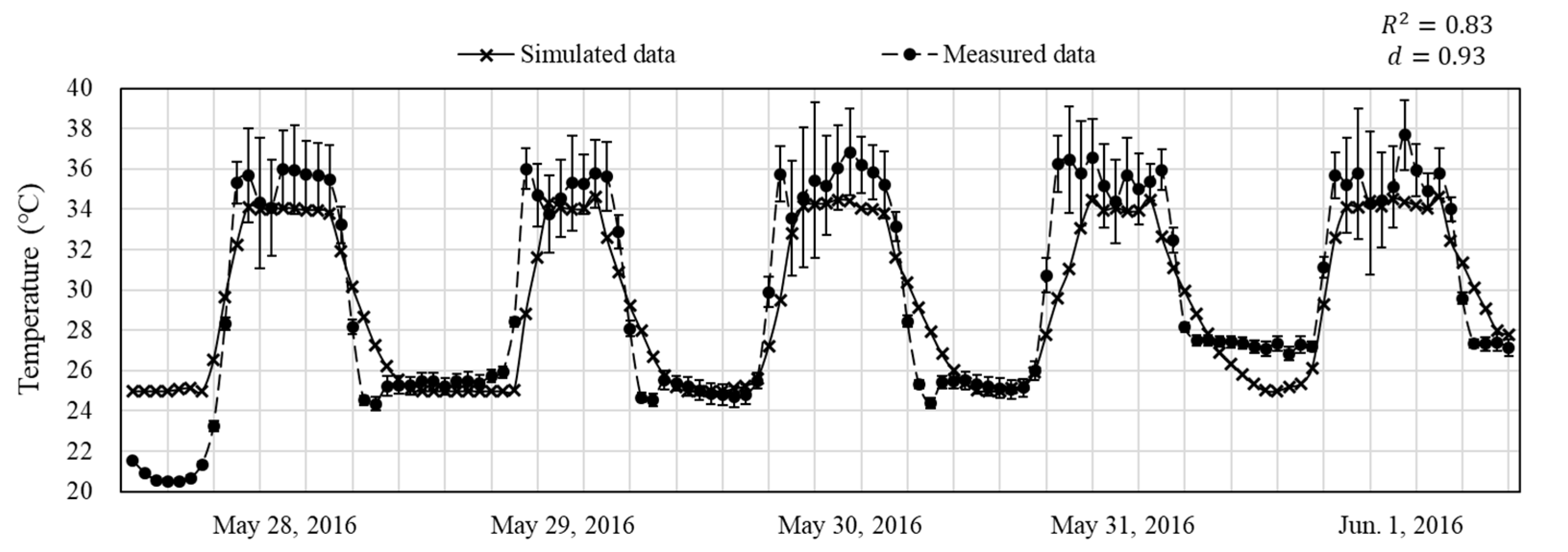
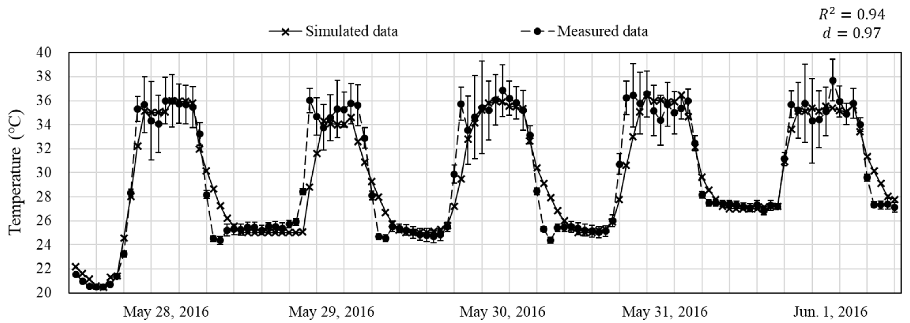
3.2.2. Validation of the Air Temperature inside the Greenhouse

To validate the greenhouse dynamic energy exchange model, the measured greenhouse internal air temperature was compared with the simulated data. The hourly internal air temperatures were calculated based on five-second intervals of measured data from fifteen locations and one-minute intervals of simulated data and compared (Figure 13). The average values of the internal air temperature at all locations were represented by dots in the figure, and the standard deviations were represented by error bars. The simulated data were the average air temperature of the crop growth space overall.
In the daytime, the internal air temperature increased due to an increase in the solar radiation, while at night, the heat pump operated based on a set temperature to maintain the internal air temperature. The simulated data typically follow the measured data; however, on the nights of the 27 and 31 May 2016, the internal air temperature differed substantially from those on other days. According to the data logger, on the night of 27 May, the heat pump did not operate, while on the night of 31 May, the set temperature of the heat pump changed from 25 °C to 27 °C. Therefore, the working schedule of the heat pump was modified, and the designed greenhouse dynamic energy exchange model was shown to provide a satisfactory estimate of the change of the internal air temperature throughout the experimental period (R2 = 0.94 and d = 0.97) (Figure 14).

3.2.3. Validation of the Air Temperature inside the Greenhouse

The simulated sensible and latent heats of crops that were obtained using the validated energy exchange model of the crop are plotted in Figure 15. Positive values of sensible and latent heats of the crops indicate energy flow from the ambient air to the crops, and negative values indicate flow in the opposite direction. As the solar radiation increased in the daytime, the energy exchange by the crops also increased, with energy flowing entirely from the air to the crops. In contrast, in the night-time, the energy exchange by the crops dropped dramatically due to the decreased amount of radiation, with the energy flow mainly due to the vapour pressure deficit between the crops and the surrounding air. Moreover, the surface temperatures of the leaves were higher than the ambient air temperature; therefore, sensible heat flux occurs from the crops to the air. According to the results of simulating the sensible heat and latent heat, the crops absorbed thermal energy at proportions of 67.0% of the latent heat and 5.3% of the sensible heat of the external radiation in the daytime. Other proportions of the external radiation were due to the photosynthesis rate stored in the plants, thermal energy rate stored in the plant, the wide spacing between pots of crops. At night-time, the crops absorbed a thermal energy of 29.54 W m−2 as latent heat and emitted a thermal energy of 9.49 W m−2 as sensible heat. This ratio for the daytime and the values of the latent heat and the sensible heat were used to analyse the energy load of the experimental greenhouse.

3.3. BES Computed Energy Load of the Experimental Greenhouse

3.3.1. Analysis of the Energy Load According to the Growth Stage

The periodic energy loads over a period of ten years were calculated. Table 6 presents the calculation results of the periodic energy loads and the external weather conditions according to the growing stage in 1 June 2014–31 May 2015 as a representative case. The cooling and heating loads mainly depended on the external air temperature and the solar radiation. The total energy load per day of the experimental greenhouse was the highest in the fruit-bearing period in winter, whereas the total energy load per day of the experimental greenhouse was the lowest in the generative growth period.
The total heating load was estimated to be about 3.1 times larger than the total cooling load over the whole growth period of 1 June 2014–31 May 2015. The cooling loads were relatively high compared to the heating loads in the generative growth period and the floral-initiation period. The heating loads were relatively high compared to the cooling loads after the floral-initiation period. As the generative growth period and the floral-initiation period of the Irwin mango start in summer, heating loads seldom occurred in these two periods. Moreover, the set temperature of the heat pump for cooling was changed from 30 °C to 20 °C as the growth period progressed; therefore, the periodic cooling loads increased from 73,693 MJ to 158,949 MJ. As the season changes from summer to autumn, the cooling loads decrease and the heating loads increase compared to the energy loads after the floral-initiation period. In the flowering period, the heating loads were higher than the cooling loads, while in the fruit-bearing period, no cooling loads were observed. For the periodic heating loads, the set temperature of the heat pump for heating was changed from 18 °C to 22 °C; hence, the periodic heating loads increased from 231,717 MJ in the flowering period to 248,483 MJ in the fruit-bearing period, which represents an increase of approximately 6%. In the fruit-growing period, the internal air temperature of the greenhouse should be maintained at more than 25 °C in the winter and spring seasons. Therefore, higher heating loads were observed relative to the cooling loads.
Table 7 lists the maximum cooling and heating loads and the times of their occurrence for each the growth stage in 2014–2015 as a representative case. The maximum cooling loads typically occurred at approximately 2:00 PM to 4:00 PM, when the external air temperature and the solar radiation were high during the day, whereas the maximum heating loads typically occurred at approximately 5:00 AM to 7:00 AM, when the external air temperature and the solar radiation level reached their lowest points of the day. As the internal air temperature of the greenhouse should be maintained in the range of 8–20 °C in spite of the summer season in the floral-initiation period, the cooling load was 456,047 kJ h−1, which was the highest among the growth stages.

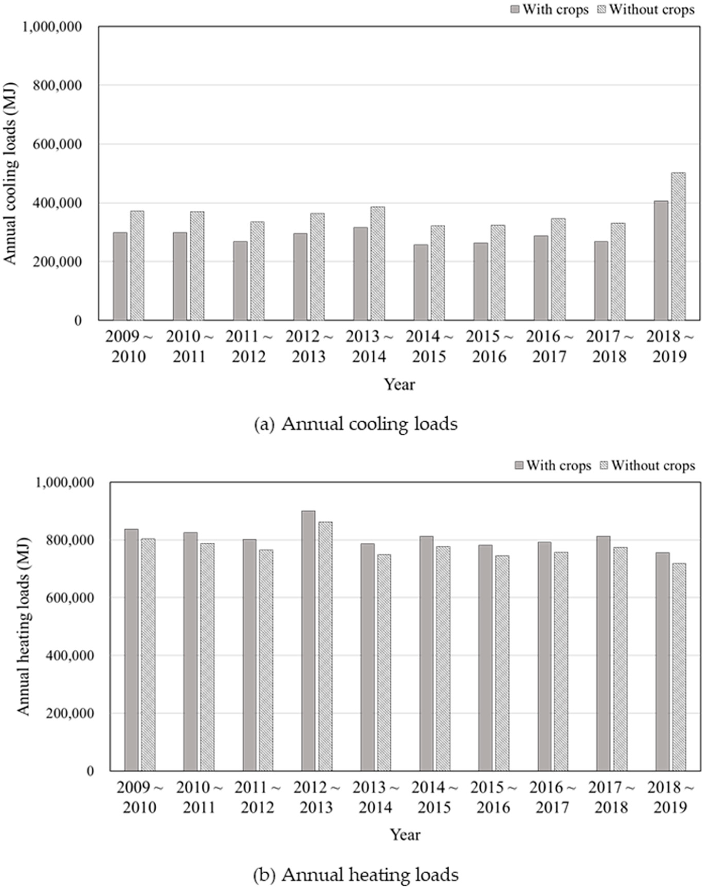
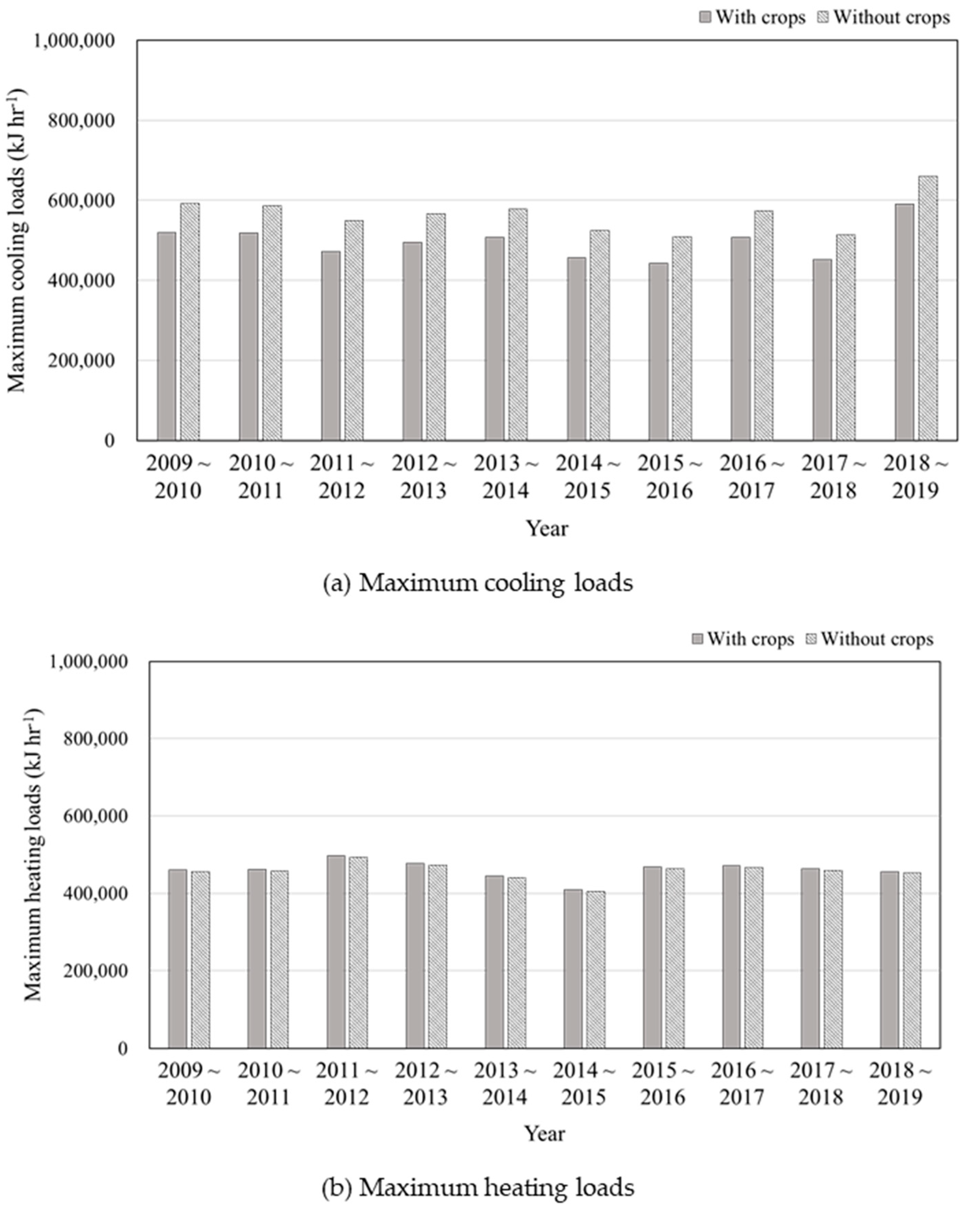
3.3.2. Analysis of the Energy Load with and without Internal Crops

Crops in greenhouses mainly absorb thermal energy in the daytime and release thermal energy at night. Many researchers who study energy balances in greenhouses emphasize that a large portion of radiation that penetrates the cladding is used for transpiration by crops [10,21,22,23,24]. The energy loads of a greenhouse can be defined as the required energy for maintaining the internal air temperature against heat transfer via conduction, radiation, and convection. If crops in the greenhouse were assumed that not to exchange energy with the ambient air, this energy will change the energy loads of the greenhouse. Therefore, to calculate the energy loads of greenhouses more accurately, the energy flow from the crops should be considered precisely. However, as stated in the literature review, most studies that simulate energy balances in greenhouses and calculate the energy loads of greenhouses do not consider the energy exchange by crops or do not consider the characteristics of cultivated crops and instead calculate the energy exchange by crops based on the findings of earlier research. In the present study, the characteristics of Irwin mangoes, such as the LAI, the stomatal resistance, and the shape of the leaves, were considered in the design of the energy exchange model of these crops. Therefore, the periodic and maximum energy loads were compared in consideration of the crops to determine the effect of the crops on the energy loads of the greenhouse. The annual and the maximum energy loads of the experimental greenhouse in consideration of the presence of the crops are plotted in Figure 16 and Figure 17. The annual and the maximum cooling loads were increased by approximately 19% and 12%, respectively, on average when assuming that the crops were not in cultivation. The cultivated crops of the greenhouse BES model that was used in this study were modelled to absorb thermal energy in proportion to the amount of external radiation during the daytime and with a constant value at night. As the cooling loads typically occurred during the daytime, the energy that was absorbed by the crops reduced the cooling loads. For the same reason, the energy that was absorbed by the crops at night increased the heating loads; therefore, the corresponding annual and maximum heating loads were decreased by approximately 5% and 1%, respectively, on average when assuming that the crops were not in cultivation.

3.3.3. Evaluation of the Design Capacities of the Heating and Cooling Systems

The maximum energy loads were calculated and used to evaluate the capacities of the heat pumps that were installed in the experimental greenhouse and to estimate the proper capacities of the cooling and heating systems (Table 8). In the last five years, the maximum cooling load was 590,258 kJ h−1, which occurred on 16 August 2019 at 3:00 PM, and the maximum heating load was 471,388 kJ h−1, which occurred on 18 February 2017 at 8:00 AM According to the Rural Development Administration of Korea, the capacity of a heat pump in a greenhouse should be set within 70% of the maximum energy load of the last five years [25]. Therefore, the proper performance of the heat pump in the experimental greenhouse is as follows: approximately 413,181 kJ h−1 for the cooling capacity and 329,972 kJ h−1 for the heating capacity. However, the performance of the heat pump in the experimental greenhouse corresponded to a maximum cooling capacity of 467,381 kJ h−1 and a maximum heating capacity of 397,267 kJ h−1. The design of the heat pump in the experimental greenhouse was excessive by approximately 54,200 kJ h−1 (13.1% of the proper cooling capacity) in terms of the cooling capacity and by approximately 67,295 kJ h−1 (20.4% of the proper heating capacity) in terms of the heating capacity. This was due to the method that was used to calculate the energy load of the greenhouse. The calculation method that was provided by the Nigerian Institution of Agricultural Engineers (NIAE) was based on a static design method and does not consider the energy exchange by crops in the greenhouse. Lee [26] determined that the maximum heating loads that were calculated via a static design method were overestimated by 37–55% compared to the maximum heating loads that were calculated via a dynamic design method. In addition, Lee [26] did not consider the crops or the thermal screen in the greenhouse; therefore, the difference between the proper performance of the heat pump as calculated via the greenhouse BES model in this study and the performance of the heat pump in the experimental greenhouse was explainable. However, the difference in the heat pump performance levels likely causes an economic loss. Therefore, it was important to calculate the energy loads of greenhouses using a dynamic design method for the realization of a more feasible heat pump design.

3.4. Comparative Analysis of the Energy Cost According to the Energy Source

The energy costs were compared according to the type of energy source, which was kerosene in this case, for the thermal effluent—heat pump system based on the calculated annual energy loads. The analysis period was the period of 2010–2014, when the temperature data of the thermal effluent were logged at the experimental greenhouse. The periodic energy loads, as calculated above, were analysed from 1 June to 31 May based on the growth stage of the Irwin mangoes; however, the energy costs were analysed from 1 January to 31 December based on the thermal effluent data. The boiler was set to use kerosene, which is the most common fuel in the greenhouses of South Korea. The caloric value of the kerosene boiler was set to 9200 kcal L−1, and the average daily oil price was used to calculate the energy cost. The price of electricity for operating the heat pump was set to 41.9 KRW kWh−1 the same for five years based on the agricultural electricity price. The annual energy usage and cost are presented in Table 9. The average energy cost when using the thermal effluent–heat pump system was found to be 68.21% lower than that when a kerosene boiler was used. Table 10 presents the average of the annual average oil price, the sea water temperature, and the thermal effluent temperature. The effect of the temperature of the sea water on the thermal effluent was minor; however, the oil price has a substantial influence on the energy savings. In 2010, when the oil price was relatively low, the energy consumption reduction ratio when using the thermal effluent—heat pump system was 58.79%, namely, more than 50%. The instability of greenhouses in South Korea, which are fundamentally vulnerable to changes in world oil prices, can be determined with the application of the thermal effluent—heat pump system based on these results.

4. Conclusions

In this study, an energy exchange model of the experimental greenhouse was designed in four parts: a model of the greenhouse structure, a model for generating the operational signals of the thermal screens, heat pumps, and vent openings, an energy exchange model of the crops, and a model of the thermal effluent–heat pump. To design the energy exchange model, field experiments were conducted to measure the structural characteristics of the greenhouse and the crop characteristics and the working schedule of the thermal screens, heat pumps, and vent openings in the greenhouse. The micro-climate of the experimental greenhouse and the transpiration rate of the cultivated crops were measured to validate the accuracy of the model. The validated model was used to analyse the periodic and the maximum energy loads. The energy loads of the experimental greenhouse were analysed according to the growth stage of the crops in consideration of the crop characteristics. The annual energy loads were used to analyse the energy cost of using the thermal effluent–heat pump system.
The designed energy exchange model of the crops was validated via comparison of the transpiration rate, which provides a satisfactory estimate of the change of the transpiration rate, throughout the experimental period ( R 2 = 0.96 and d = 0.98). The energy exchange model of the experimental greenhouse was also validated via comparison with the internal air temperature of the experimental greenhouse that was measured in field experiments. The designed model was found to be able to provide satisfactory estimates of the changes of the internal air temperature of the greenhouse ( R 2 = 0.94 and d = 0.97).
The differences in the greenhouse energy loads of the experimental greenhouse according to the presence of the crops were analysed. The maximum cooling loads were overestimated by approximately 19%, and the maximum heating loads were underestimated by approximately 5% when assuming that crops in the greenhouse did not exchange energy with the ambient air. The proper performance of the heat pump was calculated to be 363,092 kJ h−1 in terms of the cooling capacity and 328,910 kJ h−1 in terms of the heating capacity. As the performances of the heat pumps that were installed at the experimental greenhouse were 413,181 kJ h−1 for the maximum cooling capacity and 329,972 kJ h−1 for the maximum heating capacity, the capacities of the heat pumps were excessive by approximately 13.1% and 20.4%, respectively. Finally, the energy costs were compared according to the type of energy source based on the calculated annual energy loads. The average energy cost when using the thermal effluent–heat pump system was found to be 68.21% lower than that when a kerosene boiler was used.
In this study, the dynamic energy exchange between modules in the greenhouse was simulated. These results will be useful when utilizing renewable energy sources, such as geothermal heat, thermal effluent, and solar energy, in greenhouses. Since the proposed energy exchange model of crops, which considers specified crops, demonstrated high accuracy, the results of this study can provide a methodology for the design of a greenhouse energy exchange model that considers all of the major modules in the greenhouse. Additionally, the developed energy exchange model can be applied to precisely and time-dependently control the internal environments of ICT-applied greenhouse and smart farms.

Author Contributions

Conceptualization, S.-y.L., I.-b.L. and S.-n.L.; Data curation, S.-y.L.; Methodology, S.-y.L. and S.-n.L.; Software, S.-y.L.; Supervision, I.-b.L.; Visualization, S.-y.L. and S.-n.L.; Writing—original draft, S.-y.L. and S.-n.L.; Writing—review & editing, I.-b.L., R.-w.K., U.-h.Y., J.-g.K. and C.D.-V. All authors have read and agreed to the published version of the manuscript.

Funding

This work was supported by the Korea Institute of Energy Technology Evaluation and Planning(KETEP) and the Ministry of Trade, Industry & Energy(MOTIE) of the Republic of Korea (No. 20212020800050).

Acknowledgments

This work was supported by the Korea Institute of Energy Technology Evaluation and Planning (KETEP) and the Ministry of Trade, Industry & Energy (MOTIE) of the Republic of Korea (No. 20212020800050).

Conflicts of Interest

The authors declare no conflict of interest.

References

  1. Ministry of Agriculture Food and Rural Affairs. 2019 Greenhouse Status and Production of Vegetables; Ministry of Agriculture Food and Rural Affairs: Sejong, Korea, 2019. [Google Scholar]
  2. Roser, M.; Ritchie, R.; Ortiz-Ospina, E. World Population Growth. Our World in Data. 2013. Available online: https://ourworldindata.org/world-population-growth (accessed on 31 May 2021).
  3. Korea Energy Economics Institue. Yearbook of Regional Energy Statistics; Ministry of Trade, Industry &Energy: Sejong, Korea, 2019. [Google Scholar]
  4. Ministry of Agriculture Food and Rural Affairs. Guidelines for Implementing Agricultural Energy Efficiency Projects in 2015; Ministry of Agriculture Food and Rural Affairs: Sejong, Korea, 2015. [Google Scholar]
  5. Cho, S.H.; Kim, S.S.; Choi, C.Y. Study on the revision of HDD for 15 main cities of Korea. Korean J. Air-Cond. Refrig. Eng. 2010, 22, 436–441. [Google Scholar]
  6. Lee, H.W.; Diop, S.; Kim, Y.S. Variation of the overall heat transfer coefficient of plastic greenhouse covering material. Prot. Hortic. Plant Fact. 2011, 20, 72–77. [Google Scholar]
  7. Nam, S.W.; Shin, H.H. Development of a method to estimate the seasonal heating load for plastic greenhouses. J. Korean Soc. Agric. Eng. 2015, 57, 37–42. [Google Scholar]
  8. Song, S.Y.; Koo, B.K.; Lee, B.I. Analysis of Annual Heating Load Reduction Effect for Thermal Bridge-free Externally Insulated Apartment Buildings Using the Steady-state Method. J. Archit. Inst. Korea 2009, 25, 365–372. [Google Scholar]
  9. Al-Helal, I.M.; Abdel-Ghany, A.M. Energy partition and conversion of solar and thermal radiation into sensible and latent heat in a greenhouse under arid conditions. Energy Build. 2011, 43, 1740–1747. [Google Scholar] [CrossRef]
  10. Attar, I.; Farhat, A. Efficiency evaluation of a solar water heating system applied to the greenhouse climate. Sol. Energy 2015, 119, 212–224. [Google Scholar] [CrossRef]
  11. Candy, S.; Moore, G.; Freere, P. Design and modeling of a greenhouse for a remote region in Nepal. Procedia Eng. 2012, 49, 152–160. [Google Scholar] [CrossRef] [Green Version]
  12. Luo, W.; de Zwart, H.F.; DaiI, J.; Wang, X.; Stanghellini, C.; Bu, C. Simulation of greenhouse management in the subtropics, Part I: Model validation and scenario study for the winter season. Biosyst. Eng. 2005, 90, 307–318. [Google Scholar] [CrossRef]
  13. Ntinas, G.K.; Fragos, V.P.; Nikita-Martzopoulou, C. Thermal analysis of a hybrid solar energy saving system inside a greenhouse. Energy Convers. Manag. 2014, 81, 428–439. [Google Scholar] [CrossRef]
  14. Sethi, V.P. On the selection of shape and orientation of a greenhouse: Thermal modeling and experimental validation. Sol. Energy 2009, 83, 21–38. [Google Scholar] [CrossRef]
  15. Ha, T.H.; Lee, I.B.; Kwon, K.S.; Hong, S.W. Computation and field experiment validation of greenhouse energy load using building energy dimulation model. Int. J. Agric. Biol. Eng. 2015, 8, 116–127. [Google Scholar]
  16. Jiao, Z.; Yuan, J.; Farnham, C.; Emura, K. Deviation of design air-conditioning load based on weather database of reference weather year and actual weather year. Energy Built Environ. 2020, 1, 417–422. [Google Scholar] [CrossRef]
  17. Stanghellini, C. Transpiration of Greenhouse Crops: An Aid to Climate Management. Ph.D. Thesis, Wageningen University & Research, Wageningen, The Netherlands, 1987. [Google Scholar]
  18. Fynn, R.P.; Al-Shooshan, A.; Short, T.H.; McMahon, R.W. Evapotranspiration measurement and modeling for a potted chrysanthemum crop. Trans. ASAE 1993, 36, 1907–1913. [Google Scholar] [CrossRef]
  19. Monteith, J.L. Evaporation and environment. Symp. Soc. Exp. Biol. 1965, 19, 205–234. [Google Scholar] [PubMed]
  20. Willmott, C.J.; Ackleson, S.G.; Davis, R.E.; Feddema, J.J.; Klink, K.M.; Legates, D.R.; O’Donnell, J.; Rowe, C.M. Statistics for the evaluation and comparison of models. J. Geophys. Res. Oceans 1985, 90, 8995–9005. [Google Scholar] [CrossRef] [Green Version]
  21. Boulard, T.; Baille, A. Analysis of thermal performance of a greenhouse as a solar collector. Energy Agric. 1987, 6, 17–26. [Google Scholar] [CrossRef]
  22. Garzoli, K.V.; Blackwell, J. Response of a Glasshouse to High Solar Radiation and Ambient Temperature. J. Agric. Eng. Res. 1973, 18. [Google Scholar] [CrossRef]
  23. Kittas, C.; Karamanis, M.; Katsoulas, N. Air temperature regime in a forced ventilated greenhouse with rose crop. Energy Build. 2005, 37, 807–812. [Google Scholar] [CrossRef]
  24. Kittas, C.; Katsoulas, N.; Baille, A. Influence of an aluminized thermal screen on greenhouse microclimate and canopy energy balance. Trans. ASAE 2003, 46, 1653. [Google Scholar] [CrossRef]
  25. Rural Development Administration. Facility Gardening Energy Saving Guidebook; Rural Development Administration: Jeonju, Korea, 2008. [Google Scholar]
  26. Lee, S.B. Analysis and Validation of Dynamic Thermal Energy for Greenhouse with Geothermal System Using Field Data. Master’s Thesis, Seoul National University, Seoul, Korea, 2012. [Google Scholar]
Figure 1. Flow chart of the experimental procedure.
Agronomy 11 01461 g001
Figure 2. Geographic information of the Bo-ryeong thermal power plant and the experimental greenhouse.
Agronomy 11 01461 g002
Figure 3. Schematic diagram of the experimental greenhouse.
Agronomy 11 01461 g003
Figure 4. Thermal screens, crops, vent openings, air ducts that were connected with the heat pump, and circulation fans in the greenhouse. (a) Thermal screens, (b) Irwin mangoes, (c) Side openings, (d) Roof openings, (e) Air ducts connected with the heat pump, (f) Circulation fans.
Agronomy 11 01461 g004
Figure 5. Location of sensors for measuring the internal environments of the experimental greenhouse (top view).
Agronomy 11 01461 g005
Figure 6. Measurement of the stomatal resistance, the solar radiation above the plant, and the leaf temperature. (a) Measurement of the stomatal resistance, (b) Measurement of the radiation above the plant, (c) Measurement of the leaf temperature.
Agronomy 11 01461 g006
Figure 7. Measurement of the leaf area index using a plant canopy analyser.
Agronomy 11 01461 g007
Figure 8. Diagram and arrangement of the experiment equipment for measuring the transpiration rate of the Irwin mango. (a) Diagram for measuring the transpiration rate, (b) Electronics scale and computer for measuring changes in the weight of the pot, (c) Plastic wrap for sealing the pot to prevent evaporation from the soil, (d) Pyranometer that was used to measure the radiation above the plant.
Agronomy 11 01461 g008
Figure 9. Design of the BES model for calculating the energy loads of the greenhouse. (a) Model for the energy exchange in the cladding of the greenhouse, (b) Model for generating the operational signals of the thermal screens, heat pumps, and vent openings in the greenhouse, (c) Model for energy exchange by crops, (d) Model for the thermal effluent–heat pump system, (e) Final design of the BES model, in which the parts of the BES modules are connected.
Agronomy 11 01461 g009
Figure 10. The average air temperature at the centres of three heat pump air blowers and the average internal air temperatures of the greenhouse (28 May 2016–1 June 2016).
Agronomy 11 01461 g010
Figure 11. Solar radiation outside and inside the experimental greenhouse (28 May 2016–1 June 2016).
Agronomy 11 01461 g011
Figure 12. Validation results of the energy exchange module of crops by comparing the transpiration rate (28 May 2016–1 June 2016) (R2: coefficient of determination, d: index of agreement).
Agronomy 11 01461 g012
Figure 13. Validation results for the greenhouse energy exchange model in comparison with the internal air temperature of the greenhouse (28 May 2016–1 June 2016) (R2: coefficient of determination, d: index of agreement).
Agronomy 11 01461 g013
Figure 14. Modified validation results for the greenhouse energy exchange model through a comparison of the internal air temperature of the greenhouse (28 May 2016–1 June 2016) (R2: coefficient of determination, d: index of agreement).
Agronomy 11 01461 g014
Figure 15. Results of calculated latent and sensible heat fluxes through the validated energy exchange model of the crops (28 May 2016–1 June 2016).
Agronomy 11 01461 g015
Figure 16. Annual energy loads of the experimental greenhouse with versus without consideration of the crops. (a) Annual cooling loads, (b) Annual heating loads.
Agronomy 11 01461 g016
Figure 17. Maximum energy loads of the experimental greenhouse with versus without consideration of the crops. (a) Maximum cooling loads, (b) Maximum heating loads.
Agronomy 11 01461 g017
Table 1. Description of the modules in TRNSYS such as data reader, radiation processor, psychrometric calculator, sky temperature calculator, multi-zone, user-defined function, switch, and heat pump for modeling the experimental greenhouse.
IconModuleSpecification
Agronomy 11 01461 i001Data readerReads weather and sensor data to send input data to other modules
Agronomy 11 01461 i002Radiation processorInterpolates radiation data, calculates several quantities that are related to the position of the sun and estimates the insolation on surfaces of either fixed or variable orientation
Agronomy 11 01461 i003Psychrometric calculatorCalculates moist air by accepting as input the dry bulb temperature and the relative humidity
Agronomy 11 01461 i004Sky temperature calculatorDetermines the effective sky temperature for calculating the longwave radiation exchange between an arbitrary external surface and the atmosphere
Agronomy 11 01461 i005Multi-zone (greenhouse)Models the thermal behavior inside a greenhouse (heating, cooling, ventilation, and infiltration)
Agronomy 11 01461 i006User-defined functionCalculates average greenhouse internal temperature as input data for the switch module, the sensible/latent heat flux by crops, and the energy production and power consumption of the heat pump
Agronomy 11 01461 i007SwitchDetermines on/off signals for each device based on the external/internal weather conditions
Agronomy 11 01461 i008Heat pumpModels a single-stage liquid-source heat pump based on user-supplied data files that contain catalogue data for the capacity and power
Table 2. Material properties by the wall type of the greenhouse.
TypeMaterialDensity
(kg m−3)
Specific Heat
(kJ kg−1 K−1)
Thermal Conductivity
(kJ h−1 m−1 K−1)
Thickness
(m)
FrameCarbon steel78400.502154.80.0254
FloorGravel18001.0007.20.2000
Cotton15501.3380.1040.0100
Table 3. Cooling and heating performance data of the heat pump in the experimental greenhouse.
Cooling PerformanceHeating Performance
Water Temperature
(°C)
Total Cooling Capacity
(kW)
Sensible Cooling Capacity
(kW)
Power Consumption
(kW)
Water Temperature
(°C)
Total Heating Capacity
(kW)
Power Consumption
(kW)
141.3833.934.92130.088.42
539.0031.985.92537.778.47
1037.1030.426.721043.928.52
1535.2028.867.521551.008.60
2033.3027.318.322059.018.71
2531.3025.679.242568.158.85
3029.3024.0310.303077.298.99
Table 4. Optimum set temperature for operating heating, cooling, and ventilation systems according to the growth stage of the Irwin mango.
StagePeriodSet Temperature (°C)
HeatingCoolingVentilation
Generative growth06/01–08/14203027
Floral-initiation08/15–10/1982017
Flowering10/20–12/31182522
Fruit-bearing01/01–02/14223027
Fruit-growing02/15–04/14253027
Harvesting04/15–05/31253027
Table 5. Average air temperature of each measurement point in the experimental greenhouse according to day and night (28 May 2016–1 June 2016).
LocationAverage Temperature
(°C)
Average Diurnal Temperature (°C)Average Nocturnal Temperature (°C)
t129.533.325.0
t229.433.125.1
t329.833.525.4
t429.633.325.2
t529.333.124.8
t630.234.225.5
t730.033.625.7
t829.332.525.5
t929.232.625.2
t1029.633.325.4
t1131.135.525.9
t1230.534.425.9
t1329.332.525.7
t1430.534.825.5
t1530.434.825.2
Average29.933.625.4
Standard deviation0.570.920.30
Table 6. Periodic energy loads of the experimental greenhouse according to the growth stage (1 June 2014–31 May 2015).
Growth StageExternal Weather ConditionsPeriodic Energy Loads
Average Air Temperature (°C)Average Solar Radiation (kJ h−1)Cooling
Loads (MJ)
Heating
Loads (MJ)
Total Energy Load (MJ)Total Energy Load per Day (MJ day−1)
Generative growth23.464073,69313073,822984
Floral-initiation20.1521158,94968159,0172409
Flowering5.53262351231,717234,0683206
Fruit-bearing−2.1326-248,483248,4835522
Fruit-growing6.65713390254,554257,9444372
Harvesting15.878519,09978,45797,5572076
Total--257,482813,4101,070,8922934
Table 7. Maximum energy loads of the experimental greenhouse according to the growth stage (1 June 2014–31 May 2015).
StageMaximum Cooling LoadsMaximum Heating Loads
Air Temperature (°C)Solar
Radiation
(kJ h−1)
Cooling Loads
(kJ h−1)
OccurrenceAir Temperature (°C)Solar
Radiation
(kJ h−1)
Heating Loads
(kJ h−1)
Occurrence
Generative growth31.72360353,85330 July 2014 16:006.6024,6713 June 2014 05:00
Floral-initiation29.92410456,0476 September 2014 15:004.4020,76317 October 2014 07:00
Flowering13.92080104,57427 October 2014 13:00−7.70343,87922 December 2014 07:00
Fruit-bearing--- −9.50409,2858 January 2015 07:00
Fruit-growing18.62400120,73330 March 2015 14:00−6.70402,4285 March 2015 05:00
Harvesting28.42870281,88627 May 2015 14:001.40297,78117 April 2015 05:00
Table 8. Maximum energy loads for the estimation of the proper capacities of the cooling and heating systems and the evaluation of the design capacity of the heat pumps installed in the experimental greenhouse.
YearMaximum Cooling LoadsMaximum Heating Loads
Cooling Loads
(kJ h−1)
OccurrenceCooling Loads
(kJ h−1)
Occurrence
2014–2015456,0476 September 2014 15:00409,2858 January 2015 08:00
2015–2016442,74617 August 2015 15:00467,52624 January 2016 09:00
2016–2017507,25016 August 2016 15:00471,38818 February 2017 08:00
2017–2018451,79122 August 2017 15:00463,70927 January 2018 06:00
2018–2019590,25816 August 2018 15:00455,21117 February 2019 08:00
Table 9. Comparative analysis of the energy costs according to using the kerosene boiler and thermal effluent–heat pump systems.
YearBoilerThermal Effluent—Heat PumpEnergy Saving
Cost (KRW year−1)
Fuel Usage
(L year−1)
Energy Cost
(KRW year−1)
Electricity Usage
(kWh year−1)
Energy Cost
(KRW year−1)
201020,22521,534211,814887512,659 (58.79%)
201119,88325,507150,627631119,196 (75.26%)
201221,39129,793211,755887320,921 (70.22%)
201321,14729,075210,668882720,248 (69.64%)
201418,94024,610205,459860916,001 (65.02%)
Average20,31726,104198,065829917,805 (68.21%)
Table 10. The annual average of the oil price, the sea water temperature, and the thermal effluent temperature.
YearTax-Free Oil Price
(KRW L−1)
Temperature of the Sea
Water (°C)
Temperature of the
Thermal Effluent (°C)
2010107114.724.3
2011132714.424.2
2012139414.724.2
2013136514.524.4
2014130014.921.7
Average129114.623.8
Publisher’s Note: MDPI stays neutral with regard to jurisdictional claims in published maps and institutional affiliations.

