
On the Use of Sap Flow Measurements to Assess the Water Requirements of Three Australian Native Tree Species


1
School of Engineering, RMIT University, Melbourne, VIC 3001, Australia
2
Department of Plant Science and Arboriculture, Burnley College, University of Melbourne, Melbourne, VIC 3021, Australia
*
Author to whom correspondence should be addressed.
Agronomy 2022, 12(1), 52; https://0-doi-org.brum.beds.ac.uk/10.3390/agronomy12010052
Submission received: 19 November 2021
/
Revised: 20 December 2021
/
Accepted: 24 December 2021
/
Published: 27 December 2021
(This article belongs to the Special Issue Molecular Genetic Improvement of Crop Drought Tolerance)
Abstract
:The measurement of sap movement in xylem sapwood tissue using heat pulse velocity sap flow instruments has been commonly used to estimate plant transpiration. In this study, sap flow sensors (SFM1) based on the heat ratio method (HRM) were used to assess the sap flow performance of three different tree species located in the eastern suburbs of Melbourne, Australia over a 12-month period. A soil moisture budget profile featuring potential evapotranspiration and precipitation was developed to indicate soil moisture balance while the soil-plant-atmosphere continuum was examined at the study site using data obtained from different monitoring instruments. The comparison of sap flow volume for the three species clearly showed that the water demand of Corymbia maculata was the highest when compared to Melaleuca styphelioides and Lophostemon confertus and the daily sap flow volume on the north side of the tree on average was 63% greater than that of the south side. By analysing the optimal temperature and vapour pressure deficit (VPD) for transpiration for all sampled trees, it was concluded that the Melaleuca styphelioides could better cope with hotter and drier weather conditions.
1. Introduction
Plant transpiration, the evaporation of water from leaf mesophyll cells, accounts for 80% to 90% of evapotranspiration [1]. Water movement in the conducting xylem tissue of plants is passively driven by negative potential gradients generated by the evaporation of water from leaves. Measurement of xylem sap flow using heat pulse velocity-based sap flow sensors has been widely used to estimate whole-tree transpiration in the field due to the low cost of the equipment, reliability and the low power requirements [2,3,4,5,6,7]. Among commercially available sap flow instruments which depend on the measurement of temperature changes following a short pulse of heat, the Sap Flow Meter (SFM1) has been demonstrated to provide accurate and reliable measurement of zero, low and high sap flow for a broad range of plant species in various environmental conditions [8].
Many studies have monitored sap flow in trees in different locations to assess the spatial variability of sap flow around the stem. Through the study of hydraulic redistribution in a Douglas-fir tree in Brno, Czechia, Nadezhdina et al. [9] found that sap flow at the south side of the trunk was twofold lower than that on the north side and concluded the difference was attributed to a lower crown projected area on the south side. Zhang et al. [10] measured daily sap flow changes in four directions in a Populus euphratica Oliv. growing in arid northwest China and observed significant variations with explicitly higher sap flow in the south and west. Fernández et al. [11] found that sap flow in the northern roots of Olea europaea L. was 1.4 times higher than that in southern roots and Juice et al. [12] reported a positive linear correlation (r = 0.60) between sap flow rates measured on the north and south side of Quercus rubra L.
Several studies have been carried out to estimate plant water use by relating sap flow to scalar variables of plants. Hatton and Wu [13] concluded that a reliable estimation of plant canopy transpiration could be made by correlating sap flow with leaf surface area. Vertessy et al. [14] conducted in-situ cut tree experiments to determine daily water use by mountain ash (Eucalyptus regnans F.J. Muell.), and the results demonstrated that stem diameter explained 89% of the variation in mean daily sap flow.
Correlations of sap flow with meteorological parameters have been attempted in a number of studies and it has been shown that sap flow is positively correlated with air temperature [15,16]. A coefficient of determination (R2) of 0.73 indicated a strong positive linear correlation between the daily sap flow of olive trees and potential evapotranspiration [11]. In a more recent study, Juice et al. [12] showed that air and soil temperatures were excellent in correlating relative changes of sap flow in red oak trees while active radiation, vapour pressure deficit (VPD), relative humidity and photosynthetic activity had relatively smaller effects on rates of sap flow.
It is anticipated that climate change in Australia over the coming decade will lead to an increase in the frequency of extreme weather events and drier conditions with temperature rises of proximately 1 °C and 3 °C, respectively in 2030 and 2070 [17]. Rising temperatures are predicted to change terrestrial water dynamics with the difference between precipitation and potential evapotranspiration indicating a region’s aridity [18]. Understanding the physiological response of plants to climate variation is essential for assessing the ability of plants to cope with extreme weather conditions. Sap flow measurements integrate various tree traits including growth rate and conductance and could be employed as an indicator of plant health [19]. Determining periods of daily optimum sap flow of a plant will provide insights into the optimal climate for an individual tree. Determining the maximum sap flow rate over a given study period and determining the corresponding VPD and temperature will provide an indication of the ideal temperature and VPD for the growth of a species.
The performance of structures, including residential footings and masonry walls, established on expansive clays can be greatly impacted if significant amounts of water are absorbed by roots of trees nearby, resulting in localised soil shrinkage and settlement. The study reported in this paper aimed to study water use by three Australian native tree species over a period of 12 months to inform decisions about urban greening where there is a perception of danger to infrastructure and buildings as a result of planting trees in streets on clay sites. In this study, a comparison of sap flow measurements in three different tree species growing on similar soil profiles and environmental conditions was undertaken to identify which species can better tolerate hot and dry climates and pose least risk to nearby infrastructure on clay sites. Local councils could use the research outcomes to evaluate tree water consumption and develop a cost-effective planting management plan in the urban environment.
2. Materials and Methods
2.1. Description of Tree Species and Sites
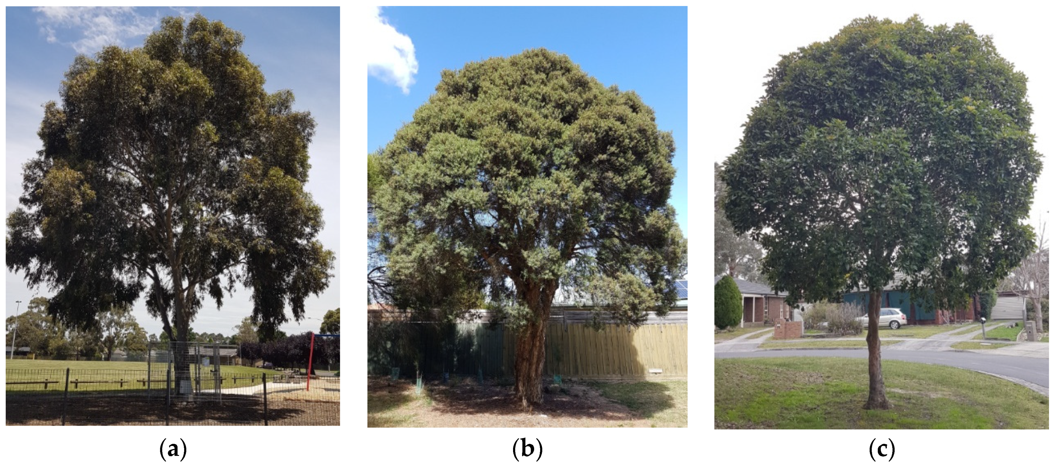
Three different Australian native tree species (Figure 1), Corymbia maculata (Hook) K.D Hill & L.A.S Johnson, Melaleuca styphelioides Sm. and Lophostemon confertus (R.Br.) Peter G.Wilson & J.T.Waterh. located at Windermere Drive, Ferntree Gully; Farnham Road, Bayswater and Centalla Green, Rowville respectively, were selected for sap flow measurements over 12 months. All the trees were situated in the same local government area (37°53′ S, 145°15′ E) in the eastern suburbs of Melbourne, the capital city of the State of Victoria. These species have been commonly and widely planted along the streets, in parks and nature reserves in south-eastern Australia. Each tree in the study was deployed with a sap flow instrument secured within a steel cage consisting of six galvanised steel panels to discourage theft and vandalism. The experimental sites are 80 m above sea level, are relatively flat and contain no evident geological anomalies. The surface geology across the sites is Quaternary aged low-level Alluvium (Qra) deposits generally composed of yellow-brown or grey mottled duplex soils.
The study area was situated in temperate climate Zone 3 [20,21], which is characterised by significant seasonal variability in the mean temperature of between 18.2 °C and 20.5 °C in the summer months and 9.6 °C to 10.4 °C during winter [22]. The annual precipitation ranged from 512.8 mm to 1108.9 mm with an average of 817.8 mm. The lowest and highest annual global solar radiation were 13.4 MJ/m2 and 15.9 MJ/m2, respectively. The meteorological data reported were obtained from 56 years of observations from 1965.
2.2. Measurement of Tree Characteristics
A photogrammetry technique was adopted in this study to characterise the trees since it is a fast and reliable means of making measurements from photographs. Photogrammetry was used to estimate tree height, crown height and mean crown diameter. A measuring pole was placed near the tree trunk while photographs were taken at azimuth 0°, 90°, 180° and 270° using a Nikon D7000 digital camera (lens: Nikon 18–105 mm f/3.5–5.6 G ED VR) attached to a tripod with a built-in spirit level to keep the line of sight horizontal. The shutter-release button was pressed when the image filled most of the frame. High-resolution images were imported into AutoCAD [23], a computer-aided design software, to determine the scale allowing tree height and crown height to be calculated. Live crown ratio (LCR) is a useful parameter that indicates tree vigour and is defined as the ratio of crown height to total tree height. A healthier and faster-growing tree generally has a larger LCR. A fiberglass tape measure was used at 1.3 m to measure the circumference of each tree trunk to allow the diameter at breast height (DBH) to be calculated.
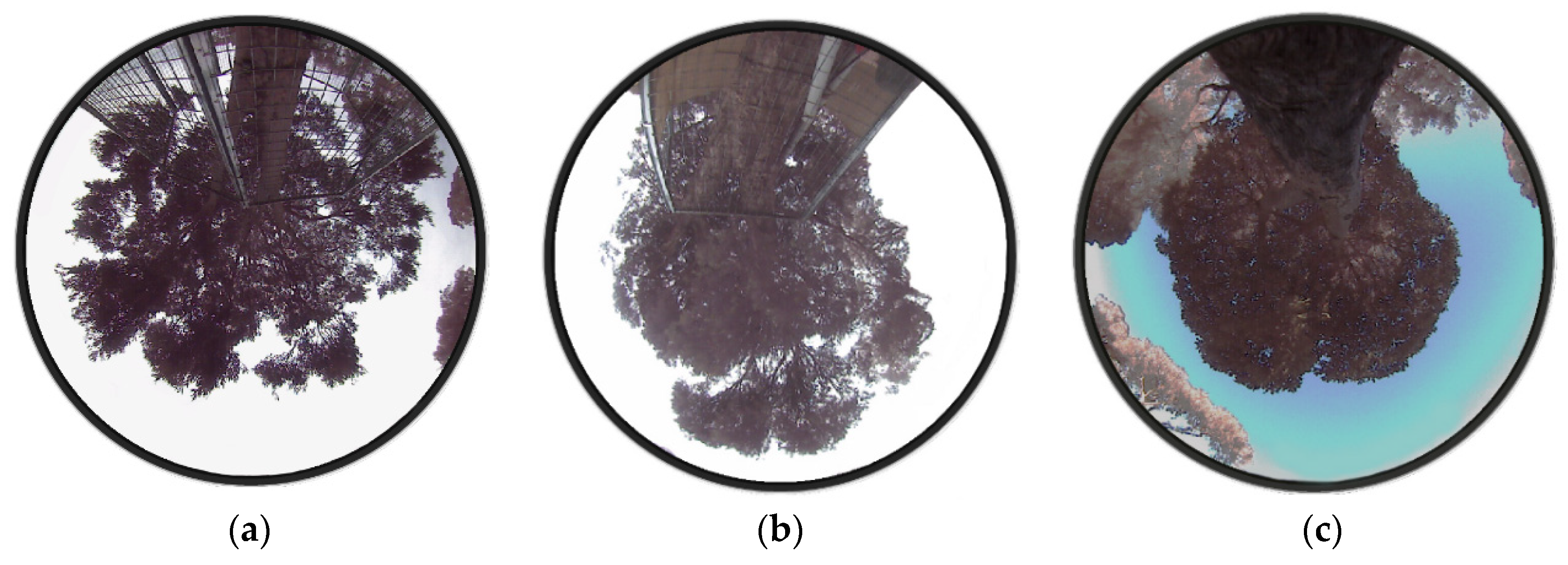
The mean crown diameter was obtained from the average length of the longest crown spread (i.e., the distance between the outmost live foliage) and the longest perpendicular spread. Hemispherical photographs (Figure 2) were collected below the canopy using the CI-110 Digital Plant Canopy Imager to include a complete crown silhouette. These images were again imported into AutoCAD to estimate the longest spread and cross-spread, allowing the outermost foliage to be located on-site and crown spreads were subsequently determined by tape measure. Tree canopy area was estimated using photogrammetry. Crown volume was determined by employing the idealised crown shape model following Coder [24], which was developed based on the standard gradient of tree crown shapes.
2.3. Determination of Wood Properties
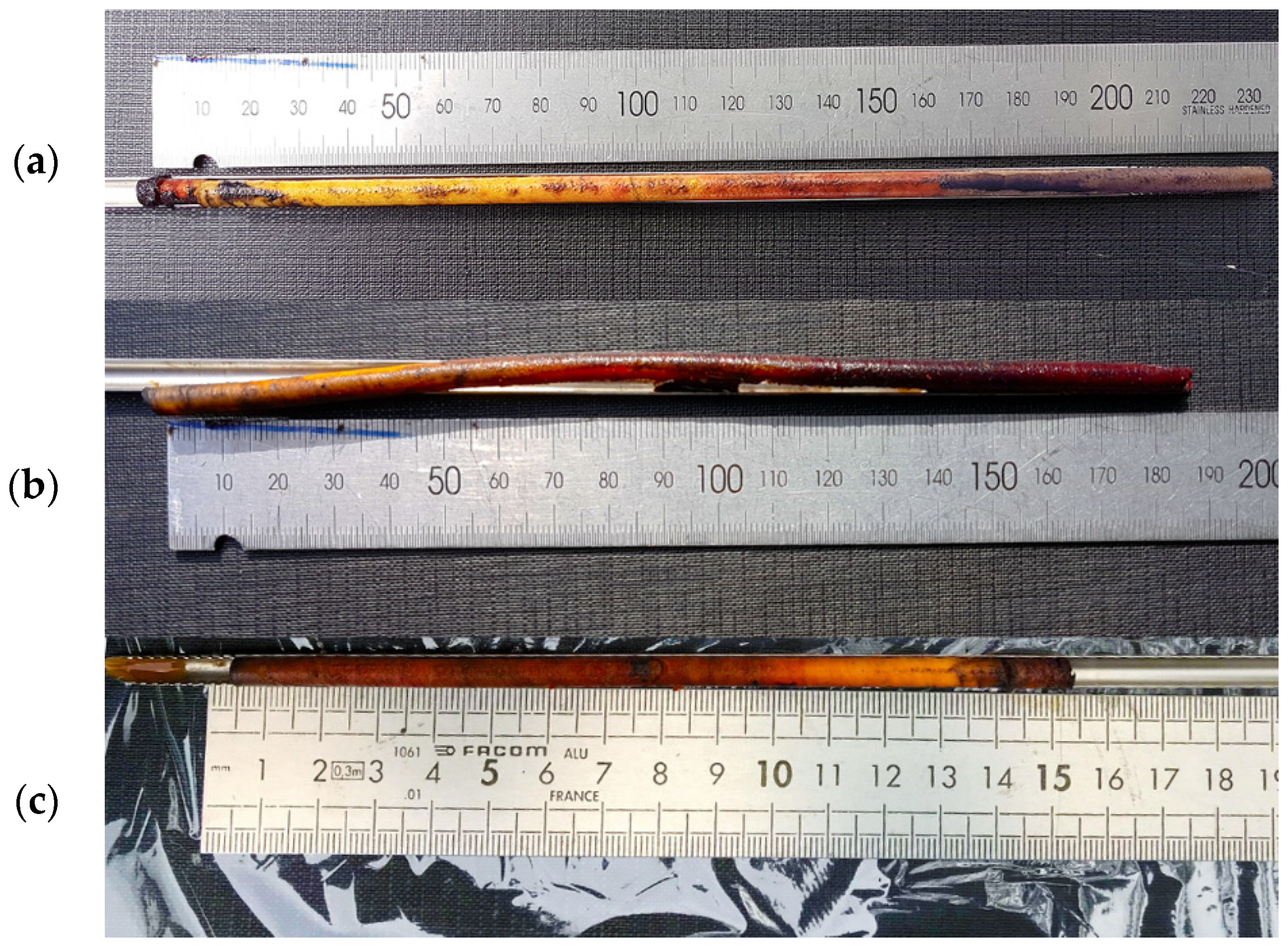
Water and nutrients are transported in the sapwood by the water-conducting xylem tissue from tree root to leaves so it is essential to determine sapwood properties such as water content and thermal diffusivity for estimating tree sap flow rates. Increment core samples representing the stem radius were extracted from sampled trees using a 400 mm long Haglöf Increment borer at breast height. Two intact cores of a diameter of approximately 5.1 mm were obtained from each tree for thermal diffusivity and moisture content determination. The sapwood and heartwood portions in the cores were turned respectively yellow and deep red colour by applying Methyl Orange (C14H14N3NaO3S) indicator dye (Figure 3), and the radial thickness was measured using a digital vernier caliper.
A bark depth gauge was employed to measure the thickness of bark at different locations at breast height and the mean is reported. Tree Basal Area (TBA) is the cross-sectional area at breast height. Dividing bark area and sapwood area by TBA yields bark percentage and sapwood percentage, respectively. Xylem radius is calculated by summing the depth of sapwood and heartwood. All measurements were made prior to the installation of the sap flow sensors
2.4. Thermal Diffusivity Estimate
Samples were sealed to prevent water loss and transported securely to the laboratory of RMIT University for sapwood density and thermal diffusivity determination. The sapwood region of the core was cut off and carefully trimmed. The diameter was measured at different points along the core length, and the mean was used. The green volume of sapwood was estimated using the formula for a cylinder. Dividing fresh weight by green volume provided the density of fresh sapwood. Cores were oven-dried at 103 °C for 48 h and subsequently weighed using a high precision scale balance.
Thermal diffusivity (k, mm2/s) is a measure of the rate at which heat spreads throughout an object and can be calculated using Equation (1) [25].
where is the density of green sapwood; is the specific heat capacity which is estimated by Equation (2) [26]; is the thermal conductivity and is calculated following Equation (3) [27]:
where is the sapwood weight after oven drying; is the sapwood fresh weight; is the specific heat capacity of wood matrix and the value of 1200 J/kg/K is used; is the specific heat capacity of water and the value of 4182 J/kg/K is adopted.
where Ks is the thermal conductivity of water; is the moisture content of sapwood; is the density of wood; is the density of water; is the thermal conductivity of dry wood matrix and is given by Equation (4) [28]:
2.5. Meteorological and Environmental Measurement
Weather parameters including mean temperature, global solar radiation, wind speed, VPD and relative humidity were obtained from a local weather observation station (Scoresby Research Institute (086104), 37°52′ S, 145°15′ E) located 2.3 km from the experimental sites. The mean temperature was determined by averaging the maximum and minimum temperature measured using wet and dry thermometers at 1.5 m above ground level. Temperature differences between the two thermometers yielded relative humidity. Wind speed was measured using cup anemometers at a height of 10 m above ground. VPD was calculated using relative humidity and temperature measurements following Monteith and Unsworth [29]. Wind speed was adjusted to a 2 m measurement height above ground level. Daily potential evapotranspiration for a tall reference crop (e.g., alfalfa) was calculated following Allen et al. [30] based on an ASCE standardised Penman–Monteith equation (Equation (5)).
where is the slope of the saturation vapour pressure-temperature relationship (kPa/°C); Rn is the net radiation (MJ/m2); G is the soil heat flux (MJ/m2); is the psychrometric constant (kPa/°C); T is the mean daily air temperature (°C) and u2 is the mean daily wind speed (m/s); es and ea are respectively saturation vapour pressure of air (kPa) and actual vapor pressure of the air (kPa); Cn is the numerator constant and Cd is the denominator constant for reference vegetation.
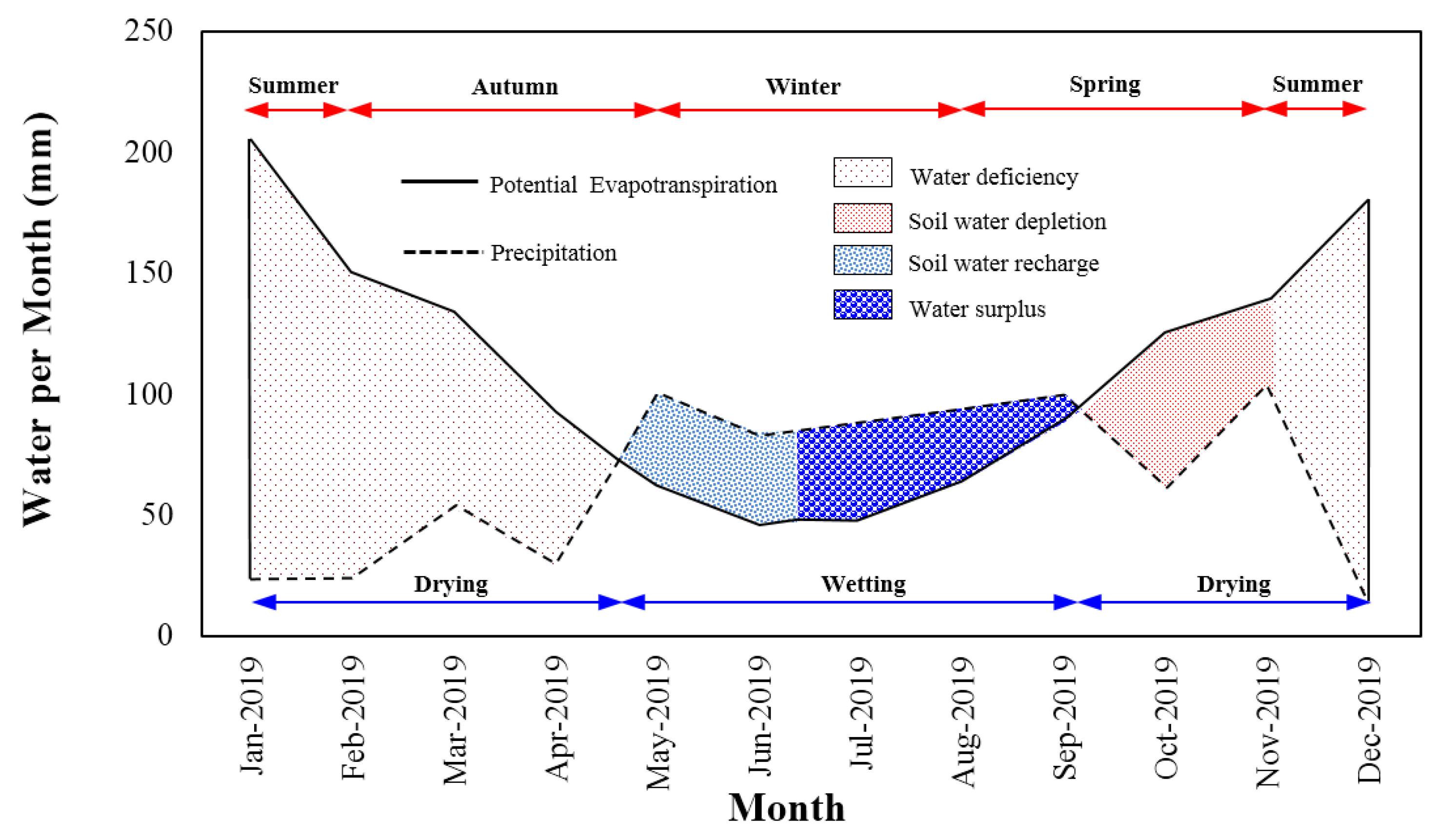
Soil Water Budget
The soil water budget is a measure of soil moisture balance which is derived from precipitation and potential evapotranspiration [31,32,33]. Water deficit occurs when the magnitude of potential evapotranspiration is greater than precipitation while soil water storage is zero. It often follows a period of soil water depletion, which takes place when the net moisture balance is below zero whilst soils have positive water storage. The positive net moisture balance leads to soil water recharge when soil storage is below the capacity of 100 mm [34] and is usually followed by water surplus which appears when precipitation exceeds potential evapotranspiration whilst water storage is at capacity.
2.6. Meteorological and Environmental Measurement
The soil-plant-atmosphere continuum (SPAC) is the water movement pathway from soil to atmosphere via the water-conducting xylem tissue of plants due to gradients of water potential. A number of monitoring instruments were deployed to measure water potential gradients at the study sites.
2.6.1. Soil Water Potential
Four in-situ soil thermocouple psychrometers (Wescor PST-55) were installed at various depths (0.4 m, 1.7 m, 2.6 m and 3.8 m) in a pre-drilled borehole near the dripline of each tree for soil water potential measurement. A 300 mm long PVC pipe with a diameter of 150 mm was used to sleeve the hole at the top of the bore casing and the pipe was capped with a cast iron inspection cover set at ground level. The PST-55 psychrometer has Dutch Weave stainless steel wire mesh enabling water vapour equilibrium with the surrounding bulk soil. Psychrometers were calibrated using sodium chloride (NaCl) solutions of known water potential in a temperature-controlled chamber prior to installation. Soil water potential is measured based on the established water vapour pressure equilibrium between the soil water and the air above soils (total soil suction). The Wescor PSYPRO Water Potential System has an accuracy between ±0.01 MPa and ±0.1 MPa and was used to take readings in the dew point mode.
2.6.2. Leaf Water Potential
Water stress suffered by plants is primarily caused by water deficit, i.e., limited soil water supply to the root system, although intense transpiration rate may also lead to stress in plants. Understanding plant water potential is important as it is an indicator of how hydrated a plant is. Stressed plants often have a low (i.e., more negative) water potential while values close to zero represent well-hydrated plants. The water potential of leaves fluctuates significantly throughout the day, which is dependent on weather conditions and stomatal behaviour. For example, leaf water potential can be affected as a result of rapid stomata closure caused by the sun being covered momentarily by a cloud. In this study, the Dewpoint Potentiometer WP4 (Decagon Devices, Inc., Pullman, WA 99163, USA) with an accuracy ranging from ±0.1 MPa to ±1 MPa was used to measure leaf water potential as it is a fast, accurate and reliable instrument [35,36] for measuring total soil water potential using the chilled-mirror dewpoint technique. The instrument was calibrated using the single-point calibration with a 0.5 Molal/kg solution of potassium chloride (KCl) as suggested by the manufacturer. Four random leaf samples were removed at the petiole junction from trees to conduct the measurement and the mean is reported. To achieve rapid equilibrium, the leaf cuticle was abraded using 800-grit sandpaper and a drop of distilled water while the leaf was still attached to the plant to minimise changes in leaf water potential.
2.6.3. Stem Water Potential
In contrast to leaf water potential which varies greatly during a day depending on weather conditions and stomatal behaviour, the water potential of stems is more stable and tends to vary depending on the overall water status of plants. Among commercially available instruments for measuring stem water potential, the PSY1 Stem Psychrometer has been commonly used in the field and has proven to be accurate and reliable [37,38,39]. This device enables continuous measurement by attaching to the sapwood of the stem. The measuring range is between −0.01 MPa and −10.00 MPa with a resolution of 0.01 MPa. The PSY1 consists of two 25 μm diametral thermocouples in series, attached to solid copper posts in the psychrometer body. The Thermocouple-C measures the psychrometric wet-bulb depression (WBD) following a Peltier cooling pulse and condensation of water on the thermocouple, while Thermocouple-S measures sample temperature by contacting the exposed xylem tissue of the plant.
In this study, the PSY1 was calibrated using six different sodium chloride (NaCl) solutions in filter paper of various concentrations (0.1, 0.2, 0.3, 0.4, 0.5, and 1.0 molality) at a controlled temperature of 25 °C. A thin layer of petroleum jelly was used to seal the gap between the cover and the psychrometer chamber. For installation, the bark and cambium were removed and the small area of water-conducting xylem was made flat to allow the instrument to be attached. The PSY1 was wrapped in a layer of cotton wool followed by two layers of aluminium foil to reduce the impact of rapid temperature changes.
2.7. Sap Flow Instrument
A Sap Flow Meter (SFM1) based on the theory of the Heat Ratio Method (HRM) was used to measure sap velocity and sap flow rate for the experimental trees as it was reliable, low maintenance and capable of measuring zero, low, high and reverse sap flow in a wide range of plant species [8,40]. The SFM1 consists of three measuring needles (one heater needle and two temperature needles), which have a length of 35 mm and diameter of 1.3 mm independently attached to the device through a cable. Two thermocouple junctions located 1.5 cm apart in the temperature needles, measure the travel of heat released by the heater needle in the water-conducting xylem tissue. SFM1 were installed on the north and south sides of each tree stem at breast height, following bark removal. A layer of petroleum jelly was smeared onto the needles prior to insertion into carefully pre-drilled holes. To enable continuous sap flow logging, the internal battery was connected to a specially designed power supply system consisting of two 12-volt batteries connected in series. These batteries were replaced regularly. Sap flow data were logged every 30 min using Campbell Scientific CR10 data loggers.
2.8. Growth Rate and Temperature
It is accepted that species with peak sap flow occurring at a later time of day will have a higher growth rate as stomata stay open for longer and increase the amount of daily carbon dioxide uptake by the plant. To determine the growth rate for the three tree species in this study, the time when the sap flow rate was at a maximum each day was compared with the daily maximum VPD.
To assess which species could better cope with predicted hotter weather due to climate change, the daily sap flow volume of individual species was calculated for 12 months (rain days were removed). The top 5% of data were used to conduct the analysis as the plant is at its most optimal physiological condition when sap flow is at its highest. The VPD and temperature corresponding to the top 5% of sap flow were determined.
3. Results and Discussions
3.1. Tree Information
Characteristics of the three different tree species used in this study are provided in Table 1. The C. maculata was significantly taller than the other two species and possessed the largest canopy as seen by the crown height and mean crown diameter. A larger LCR of 0.9 was determined for both C. maculata and M. styphelioides, indicating an increased potential for survival and reproduction. It is noted that the crown volume of M. styphelioides and L. confertus were respectively 76% and 87% smaller than that of C. maculata.
3.2. Wood Properties
The wood properties of the tree species are presented in Table 2. It is evident that the sapwood area of individual trees varied substantially. A greater bark depth was measured for M. styphelioides which also had the highest bark percentage. Almost half of the TBA is occupied by sapwood for C. maculata and L. confertus.
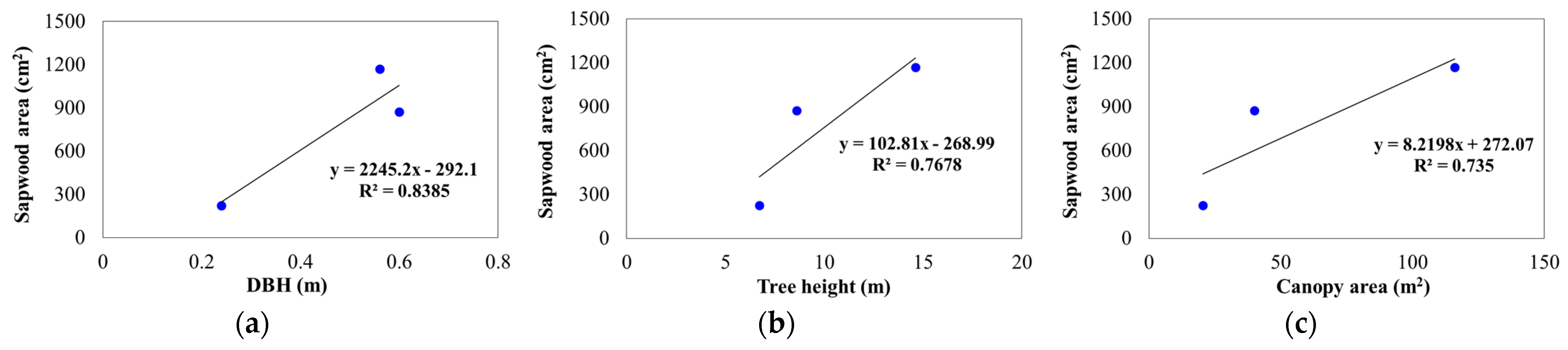
The coefficient of determination (R2) was used to correlate sapwood area to DBH, tree height and canopy area, and a reasonably strong positive linear relationship was obtained for the 3 data points, as shown in Figure 4. It is worth emphasising that almost half of the TBA was occupied by sapwood for L. confertus box and C. maculata.
Essential parameters in determining k of sapwood for different tree species are presented in Table 3. It can be seen that k ranged from 0.22 to 0.26 mm2/s which lies within the range prescribed by the threshold from 0.14 mm2/s for water at 20 °C to 0.40 mm2/s for dry wood [41]. Higher moisture content in sapwood can lead to a greater value of k.
3.3. Meteorological Measurement
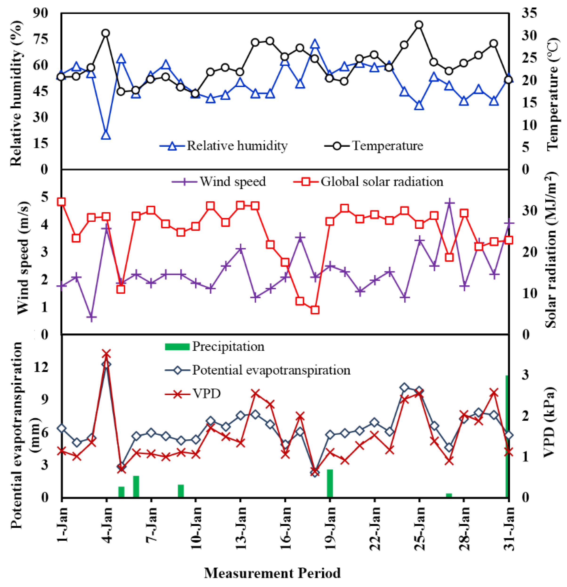
Meteorological parameters including global solar radiation, mean temperature, relative humidity, wind speed, VPD and ETref over a 31-day period in summer (the month of January) at the study sites are presented in Figure 5. The measured variables varied greatly daily and such variations are highly intercorrelated. Figure 5 clearly shows that the study sites experienced an arid summer month with a daily mean temperature of 23.4 °C and total precipitation of 18.4 mm which contributes only 2.6% of the annual rainfall. It can be seen that the soil was driest on the 4 January due to a larger VPD and evapotranspiration rate associated with low relative humidity and high temperature. It is noted that not all of the rainfall events occurring during the monitoring period would lead to decreases in global solar radiation and VPD. This observation is different from the study conducted by Nadezhdina et al. [9] which found a significant decrease for these two variables during a rain event.
A soil moisture budget profile featuring precipitation and potential evapotranspiration for the study site over 12 months (1 January 19–31 December 19) of monitoring is depicted in Figure 6. It can be seen that a deficit had occurred in summer until late autumn followed by water recharge before water surplus occurred from mid-winter to early spring as a result of frequent rainfall events and low evapotranspiration rates. Soil depletion commenced thereafter due to a higher water uptake rate by vegetation prior to a deficit occurring again during early summer. Figure 6 also presents seasonal drying and wetting. The study site was arid with only four dominant wetting months throughout the year.
3.4. Soil-Plant-Atmosphere Continuum
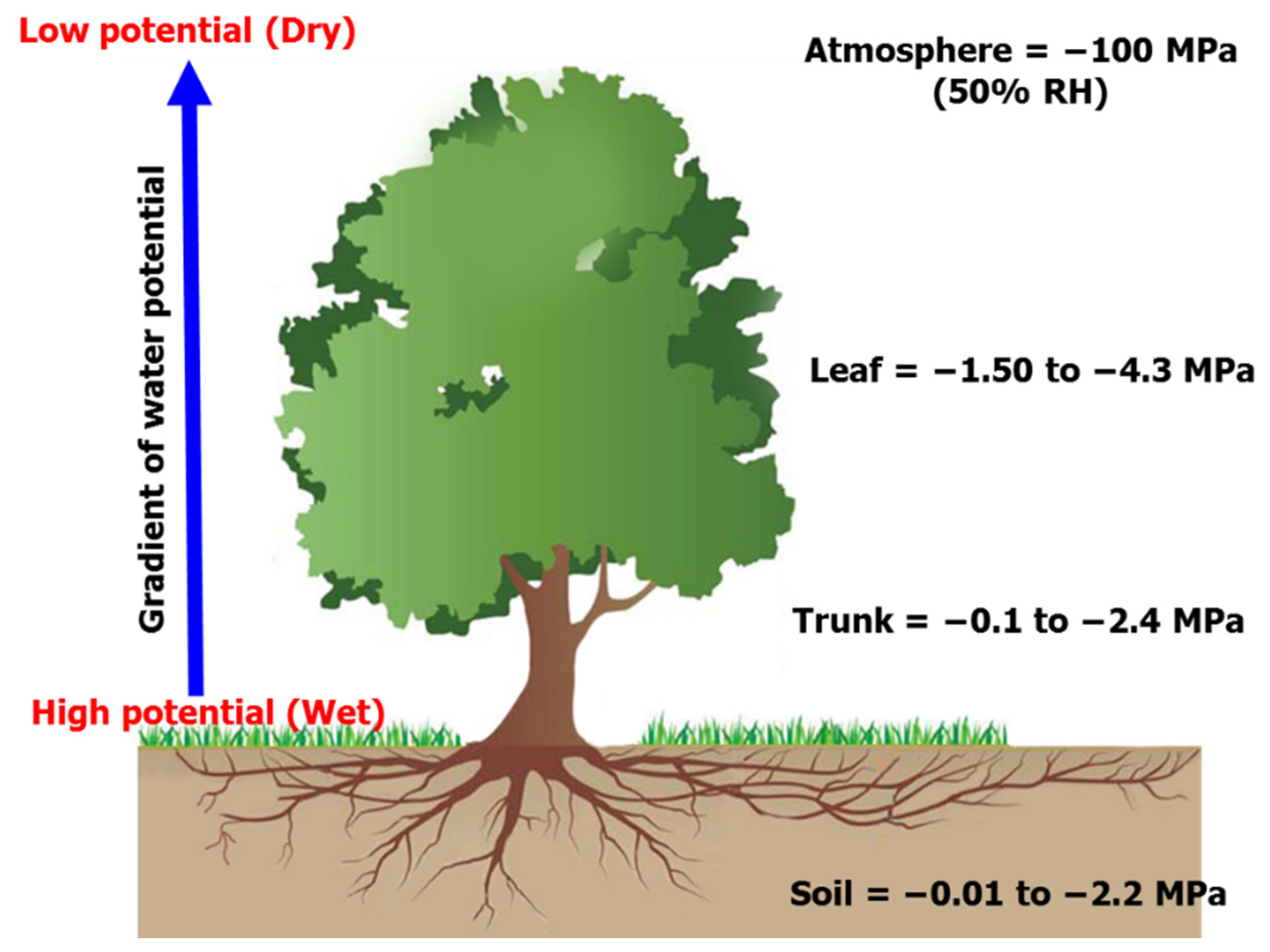
Figure 7 presents a schematic example of the soil-plant-atmosphere continuum (SPAC) established in close vicinity to the L. confertus based on 12 months of monitoring of soil (depth varies from 0.4 m to 3.8 m), stem and leaf water potential. It can be seen that total soil water potential varied from −0.01 MPa to −2.2 MPa, through the stem which had an intermediate lower value than the soil but higher than the leaves, to the atmosphere which had the lowest potential. It is noted that a typical water potential for dry air is approximately −100 MPa at 50% relative humidity although it varies based on both temperature and humidity. The reduced water potential gradient leads to passive water movement from the soil to atmosphere via water conducting xylem tissue. It is worth noting that, in this example, the upper boundary of the measured total soil and stem water potential is very similar, which might be explained by the close proximity of the measurement position of stem water potential at breast height.
3.5. Sap Flow Measurement
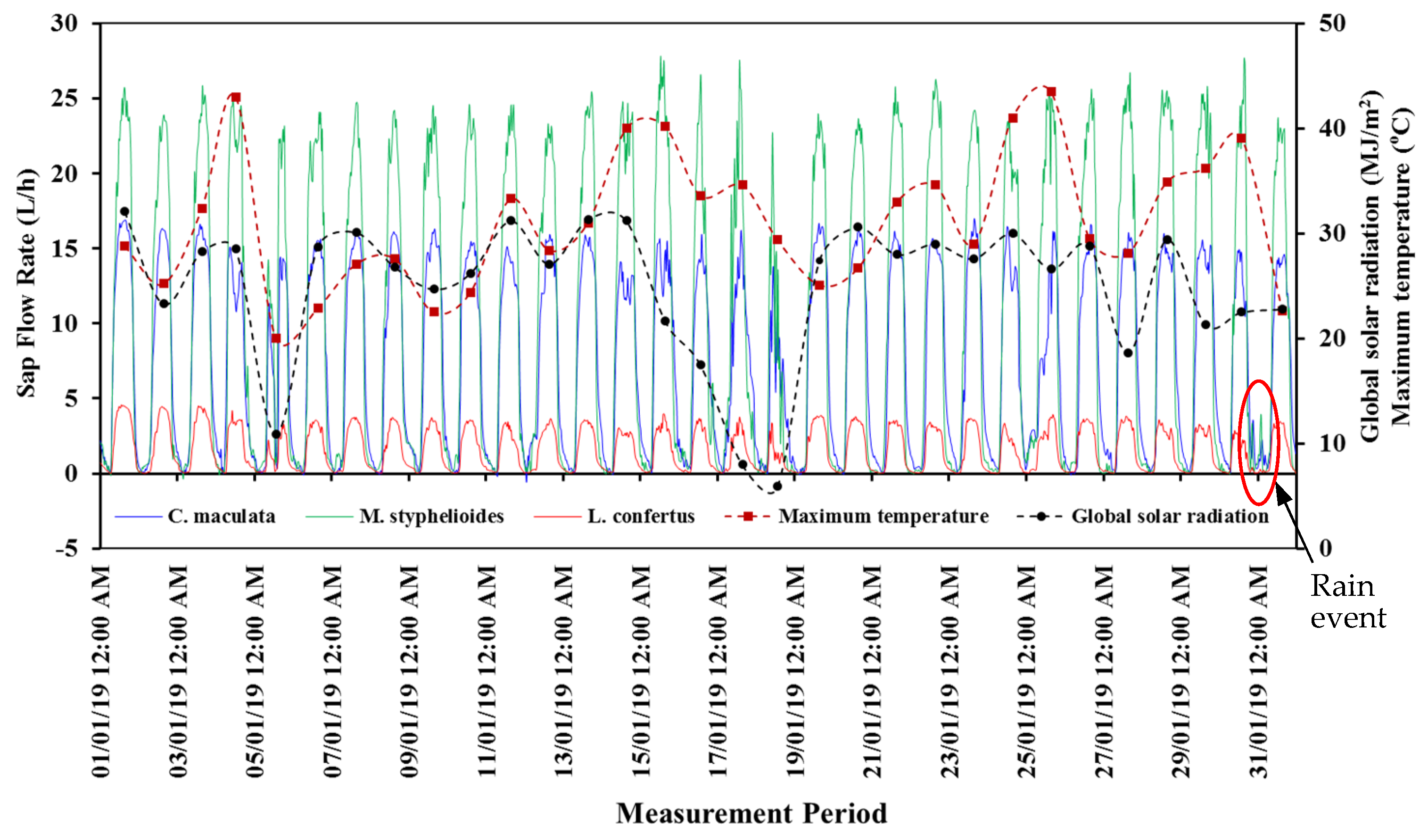
A comparison of daily sap flow from the north side of the three trees across January 2019 is presented in Figure 8. It is apparent that sap flow exhibited a ‘bell-shaped’ curve daily, where noticeable sap flow increases occurred in the morning with fluctuating peaks in the early afternoon in response to changing light conditions and evaporative demand prior to a gradual reduction which stabilised around zero flow at midnight. The daily sap flow patterns are similar to the sap flow measurements reported for individual trees by many researchers [5,6,26,36]. Substantially higher sap flow rate was observed in daytime compared to nocturnal water uptake. Loustau et al. [42] found that night-time sap flow only contributed 12% of the daily total transpiration.
Weather parameters including maximum temperature and global solar radiation are also plotted in Figure 8 to compare with tree sap flow. It is evident that a marked sap flow decrease occurred on the 18 January for all trees and this is most likely due to the low global solar radiation of only 5.9 MJ/m2, which is far below the monthly mean of 25 MJ/m2. There were five days (4th, 14th, 15th, 24th and 25th) that exceeded 40 °C over January. The resulting sap flow for all species declined compared to the previous day, possibly due to stomatal closure caused by heat stress. It is noted that sap flow for all trees fluctuated dramatically in the early morning of the 31 January, which can be attributed to the intensive rainfall event of 11.2 mm, which contributed 61% of the monthly total.
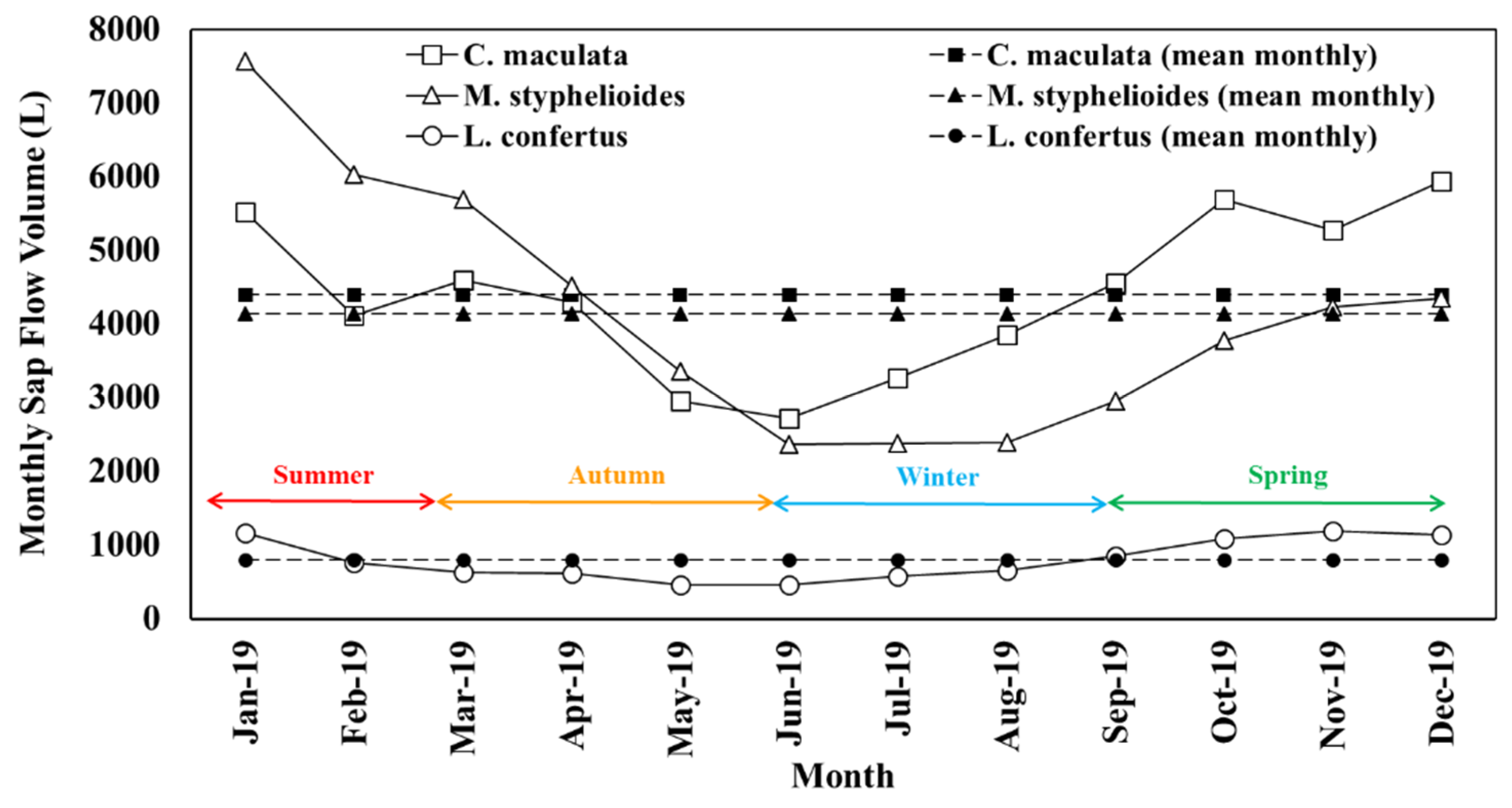
Figure 9 presents a similar pattern of variation of monthly sap flow volume on the north side for the three tree species despite significant discrepancies of the daily amount of water absorption for individual trees depending primarily on weather conditions. It is apparent that larger sap flow volume occurred in spring months for C. maculata and L. confertus with the maximum water use in October and November, respectively. This finding shows that water use by C. maculata was 62–65% higher than the water consumption measured by Sun et al. [36] for the same species during spring. M. styphelioides had its highest transpiration rate during January in summer. All sampled trees had their lowest water demand in June and a significant increase in late winter.
It is worth mentioning that although the annual cumulative sap flow volume of C. maculata is the highest with mean monthly water use of 4399 L, however, on a canopy area basis, this tree is found to be a miserly water user with the lowest water uptake rate of 1.25 mm3/mm2/day compared to L. confertus and M. styphelioides using respectively 1.28 mm3/mm2/day and 3.40 mm3/mm2/day. It is interesting to note that the M. styphelioides consumed almost the same amount of water (2380 L) to survive in winter months which is 43% lower than the mean monthly consumption. The total amount of water uptake by M. styphelioides is 26% higher than the C. maculata in the first five months of the year, although the mean monthly water use is 264 L lower due to the substantial rise in water demand by C. maculata from late autumn.
Sap flow in the North and South Sides of the Tree Trunk
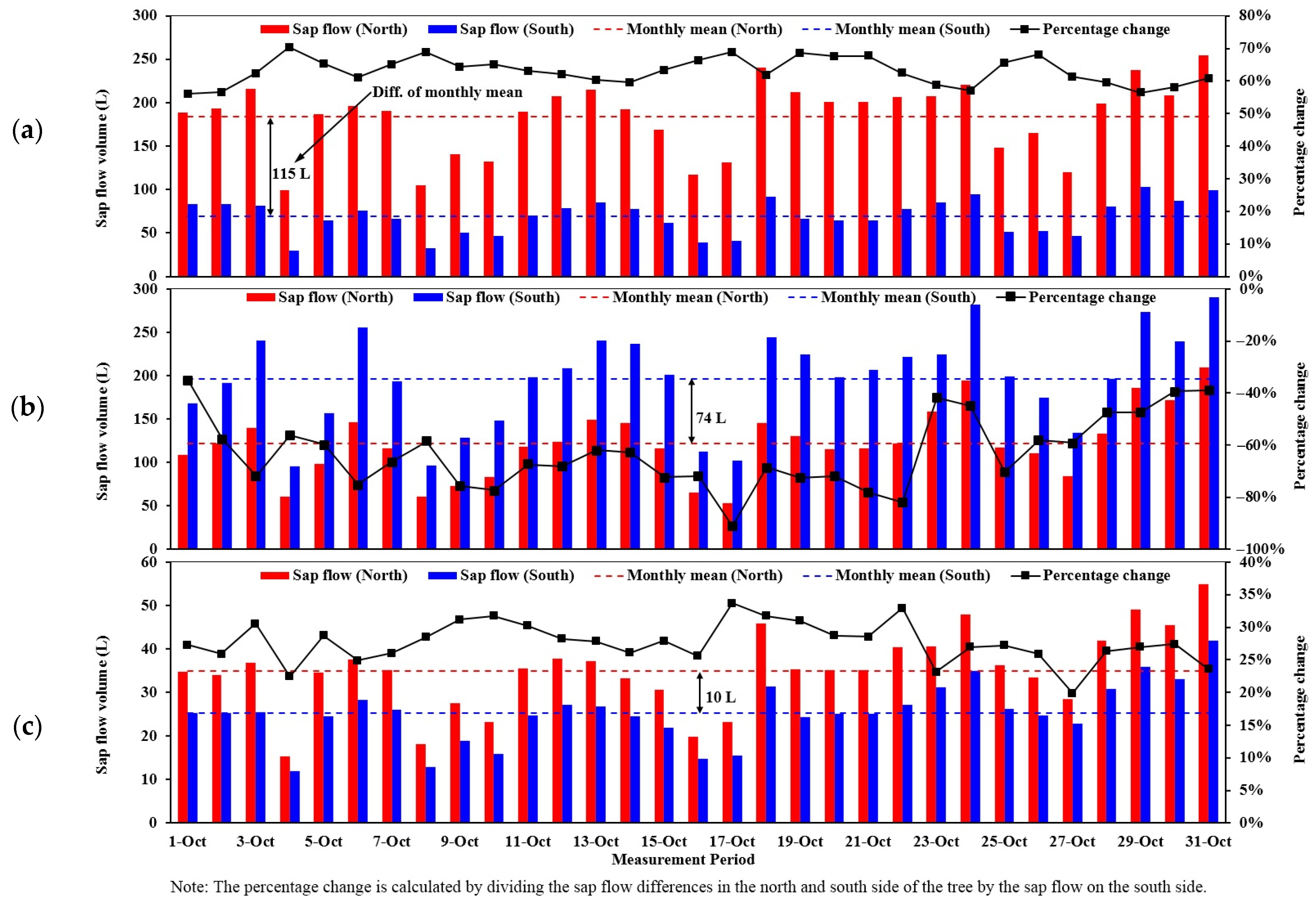
The daily sap flow volume on the north side of the trunk was compared with the south side measured at the same radial depth by the SFM1 for the three species through October and the result is depicted in Figure 10. It was found that sap flow volume varied greatly at the same depth but at different locations from day to day for individual trees. The C. maculata consumed a substantial amount of water daily on the north side which was 56–70% higher than that of the south side. This trend is similar to the observations by Nadezhdina et al. [9] that sap flow on the north side of Douglas-fir was twice that on the south side. The daily water use on the north side of the L. confertus, on average, was 28% greater than that of the south side, although the difference of the monthly mean was only 10 L which is the smallest when compared to 115 L and 74 L for C. maculata and M. styphelioides, respectively. Interestingly, the average percentage change of daily sap flow volume between the north and south side of the M. styphelioides was the same as that of the C. maculata (63%), however southern sap flow volume of this tree was significantly higher, which is in stark contrast to the other two trees. The discrepancies of sap flow volume at different sides of a tree could be attributed to an uneven interception of solar radiation or uneven crown canopy distribution. It is worth noting that the C. maculata had experienced the greatest variation of daily sap volume between the north and south sides of the tree ranging from 70 L to 155 L with the mean () of 115 L (23).
3.6. Relationship between Tree Sap Flow, Meteorological Parameters and Stem Water Potential
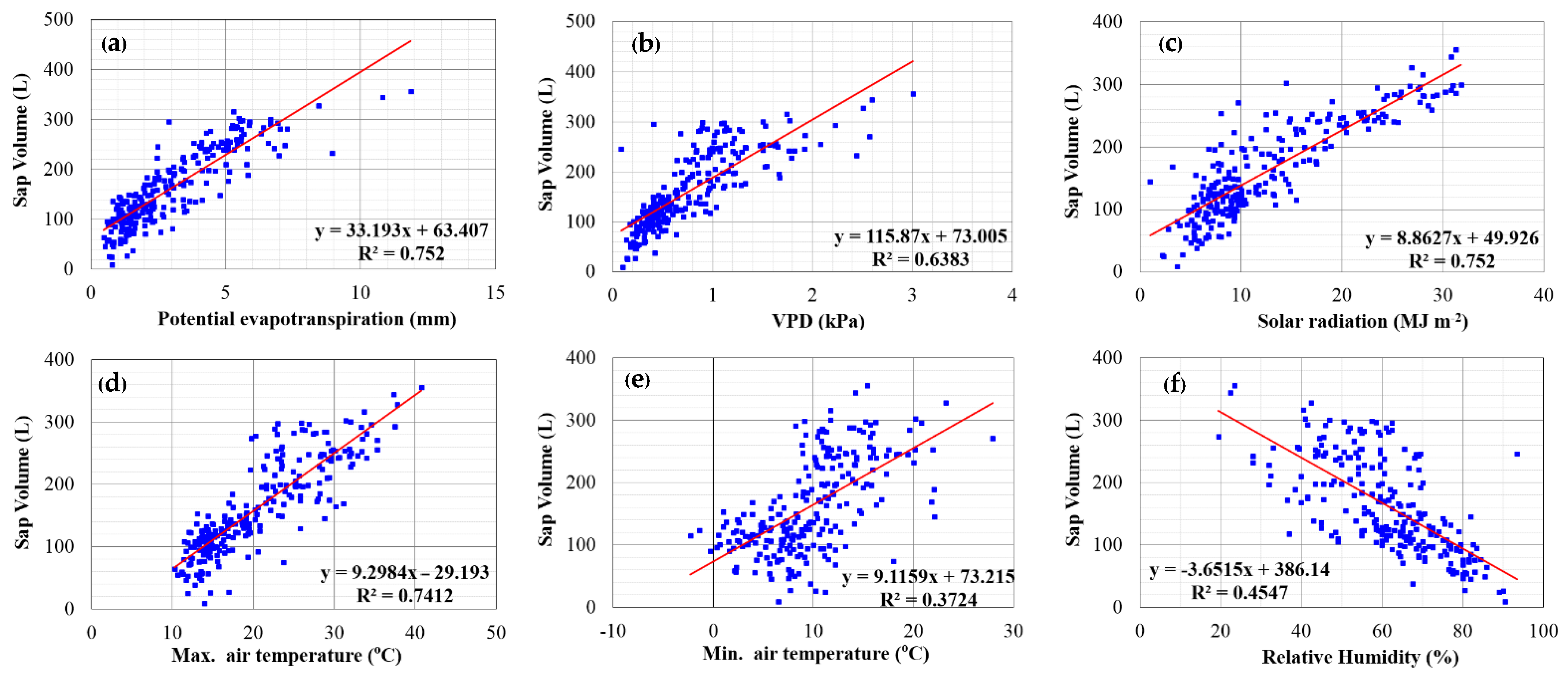
An attempt was made to correlate the daily sap flow volume at the north side of M. styphelioides to various weather parameters, including relative humidity, solar radiation, VPD, potential evapotranspiration and maximum and minimum air temperature over 12 months. The linear regression analysis in Figure 11 revealed potential evapotranspiration and solar radiation were positive in correlating relative changes of sap flow volume of plants with the best R2 of 0.75. This finding is very similar to the R2 of 0.73 obtained for the sap flow—potential evapotranspiration correlation for olive trees [11]. Contrasting the sap volume—relative humidity correlation in Figure 11f which showed an inverse linear relationship, all other weather data (Figure 11a–e) indicated a positive correlation with sap volume where an increase in these parameters can lead to a rise in sap volume. It can be seen from Figure 11e that the smallest R2 of 0.37 was for the correlation between sap volume and minimum temperature, which is not as strong as the maximum temperature–sap volume relationship which explained 74% of the variation in sap volume. The stronger correlation could be attributed to faster sap flow at higher temperatures. It is noted that sap flow remained almost constant when potential evapotranspiration and VPD reached 5–6 mm/day and 0.8–1 kPa, respectively.
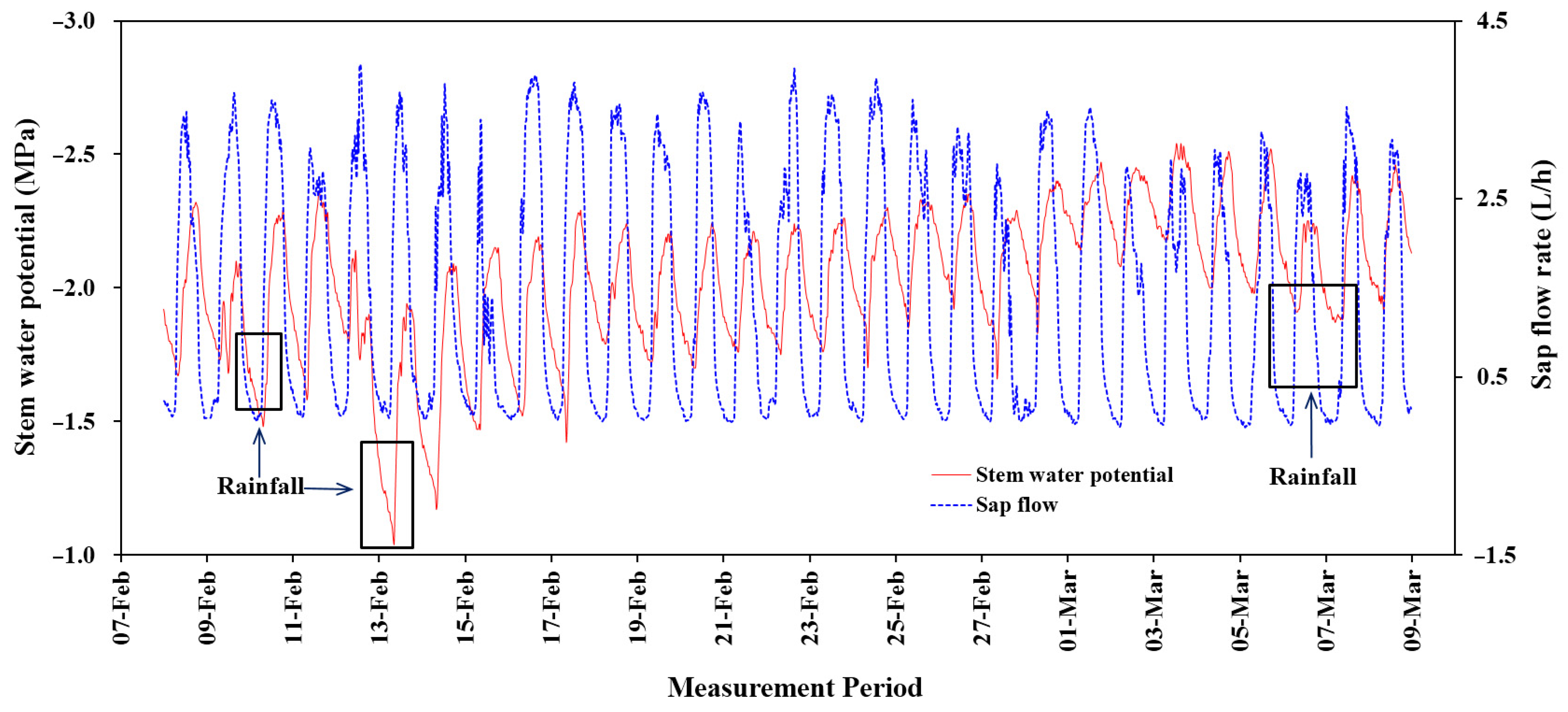
Figure 12 presents the comparison between stem water potential and sap flow rate at the north side of the L. confertus half-hourly for 30 days throughout the seasonal transition from summer to autumn. It is evident that the tree suffered a regular cycle of moisture stress with water potential ranging from −1.04 MPa just a few hours before sunset (5:30–7:30 p.m.) to −2.54 MPa after sunrise. Water stress began to develop following a rainfall event on the 10 February and a subsequent substantial increase to a maximum of −1.04 MPa on the 13 February due to intense precipitation. The tree experienced an increasing water deficit, with the daily minimum declining gradually from −2.09 MPa to −2.33 MPa over the next 19 days as there was no night-time recovery or rehydration owing to limitations of water supply. Tree water stress was relieved by two consecutive days of rainfall, leading to a water potential of −1.87 MPa on the night of the 7 March. Photosynthesis can slow or even stop due to prolonged high levels of water stress in the stem which may cause reduced or delayed growth.
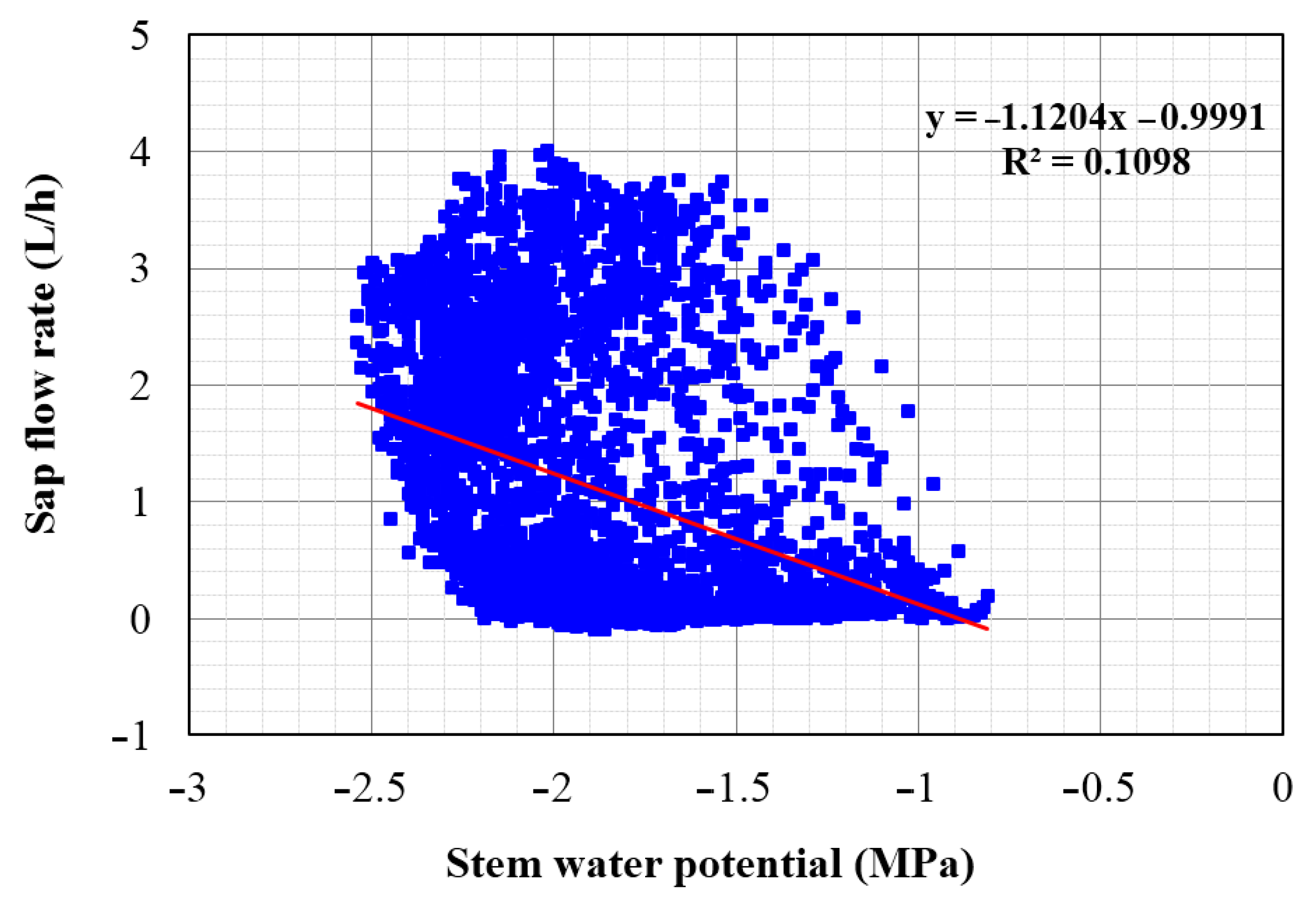
Figure 12 shows the hysteresis loops of sap flow rate and stem water potential. The water potential decreased markedly in the afternoon and dropped to its minimum a few hours after the maximum sap flow rate had been reached, which was most likely due to stomatal closure caused by water stress. Figure 13 shows the lack of linear correlation between the rate of sap flow and stem water potential on a half-hourly basis. The linear regression indicated a weak negative linear relationship.
3.7. Tree Performance
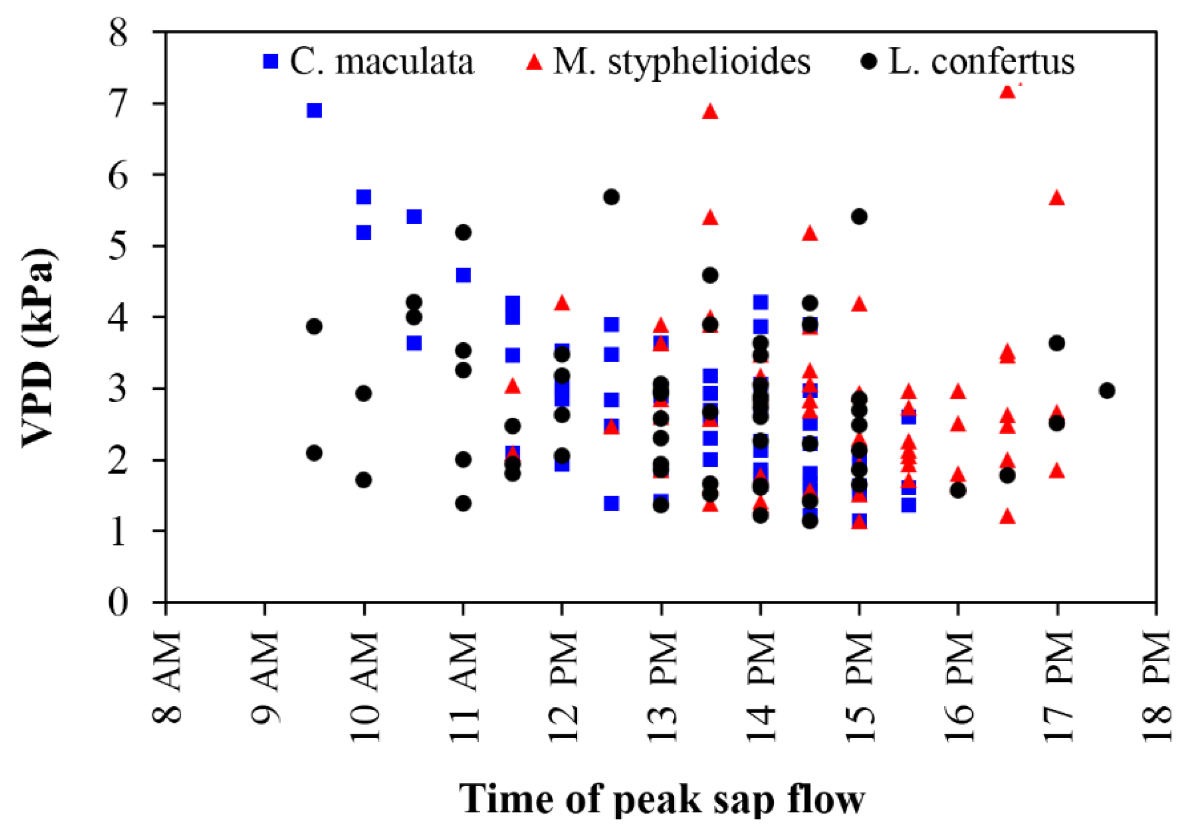
The time of occurrence of daily maximum sap flow was plotted against the corresponding daily maximum VPD during summer in Figure 14. It can be seen that the sap flow rate of the C. maculata peaked early in the morning on days of high VPD compared to the other two species, of which the sap flow reached a maximum later in the afternoon.
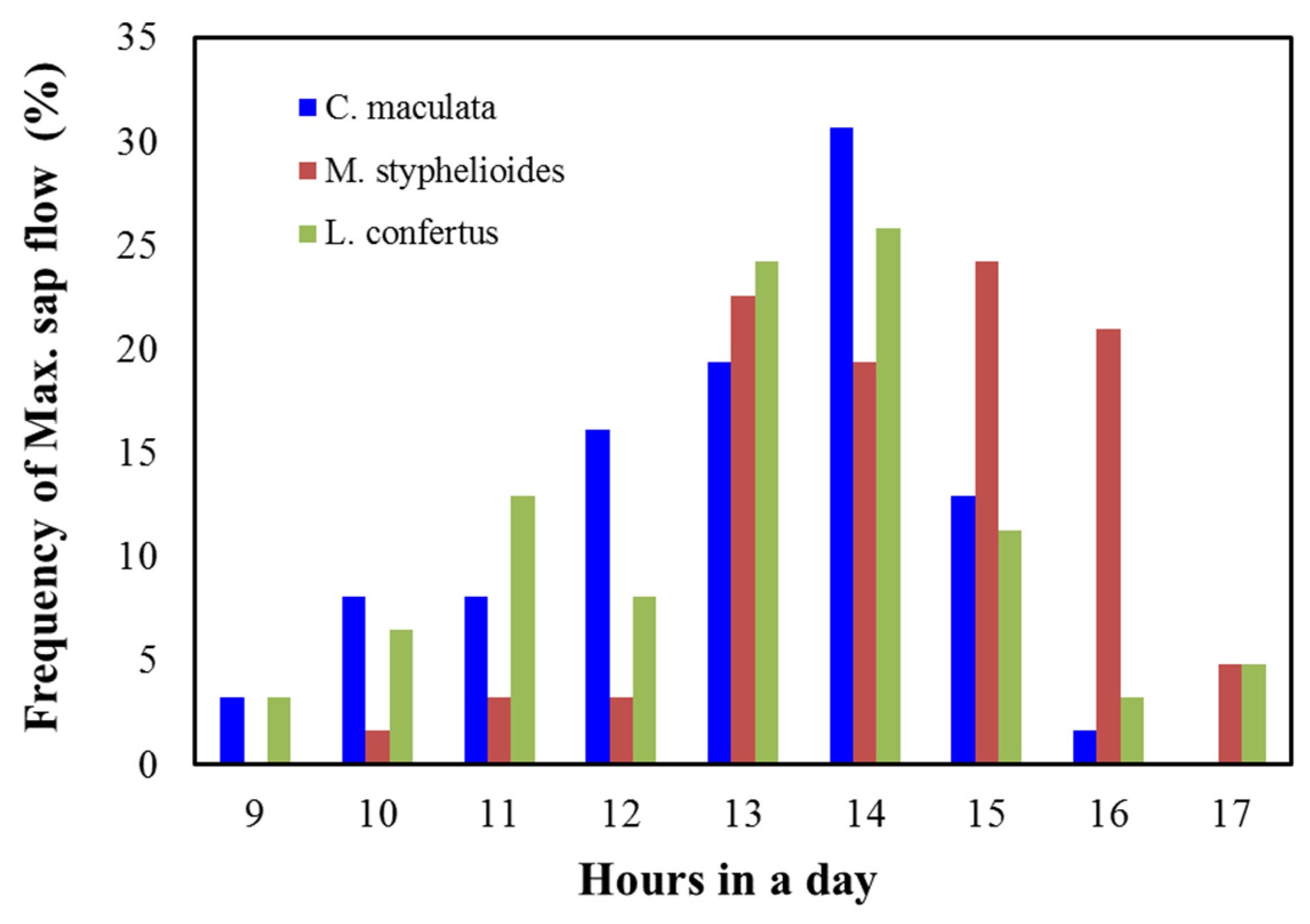
The frequency of occurrence of maximum sap flow during the day (closest hour) over the summer months is presented in Figure 15. It is evident that the maximum sap flow for both C. maculata and L. confertus occurred between 2 and 3 p.m. on 31% and 26% of all days, respectively, over the monitoring period. It was found that the most frequent occurrence of maximum sap flow of about 25% was between 15 and 16 h for M. styphelioides indicating that the tree absorbed more carbon dioxide from the atmosphere and potentially had a higher photosynthetic rate which could contribute to an increase in growth rates.
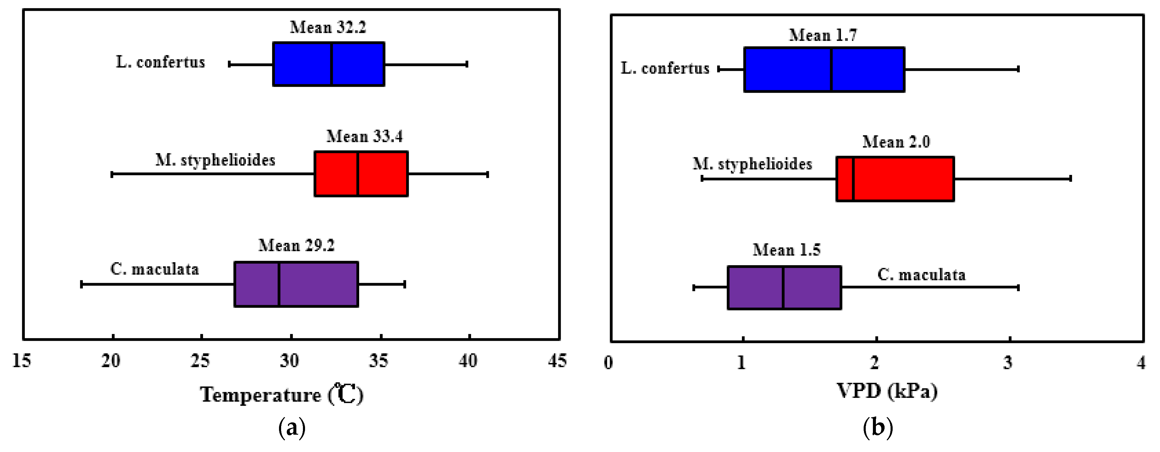
Figure 16a presents the variation in optimal temperature for each species. A significant temperature difference was found between species with M. styphelioides having the highest mean (±S.D.) optimal temperature of 33.4 °C (±5.3), indicating this species is more suited to a hotter atmosphere and has a greater tolerance to heat. Compared to the other two species, the C. maculata is less heat tolerant with a mean optimal temperature of 29.2 °C (±5.2). The mean optimal VPD for all three species varied from 1.5 kPa (±0.7) to 2.0 kPa (±0.8) (Figure 16b). The results show that C. maculata has less tolerance to a drying environment than the other two species. M. styphelioides has a greater ability to maintain fast sap flow under a drier atmosphere allowing the tree to exchange a given amount of water for additional carbon dioxide to perform photosynthesis and thus increasing growth rates.
4. Conclusions
Sap flow instruments based on HRM were employed to evaluate water use of three tree species located in the eastern suburbs of Melbourne through the monitoring of sap flow over a 12-month period. The measured daily sap flow exhibited a typical ‘bell-shaped’ curve for all trees with substantially higher sap flow rates occurring during the day compared to night-time water use. The monthly sap flow volume comparison for the three species clearly showed that C. maculata outperformed the other two trees in terms of whole-plant water use and transpired substantial amounts of water in the spring months. The daily sap flow volume on the north and south sides were compared and it was seen that water use on the north side of the C. maculata and L. confertus, on average, was respectively 63% and 28% greater than that on the south side, while the M. styphelioides transpired a significantly higher amount of water on the south side than on the north side.
Through the analysis of sap flow during the day over summer months, it was found that sap flow peak rates in M. styphelioides occurred more often later in the day compared with the other two species, allowing the tree to uptake more carbon dioxide which could potentially contribute to an increase in growth rate. The optimal temperature and VPD were determined from sap flow measurements to assess the potential of species in coping with the expected hotter and drier weather under climate change. The results revealed that the M. styphelioides had the highest mean (±S.D.) optimal temperature of 33.4 °C (±5.3) and VPD of 2.0 kPa (±0.8), indicating that this species is better suited to hotter and drier weather conditions and has a greater tolerance to heat extremes.
Author Contributions
Conceptualisation, X.S. and J.L.; methodology, X.S.; software, X.S.; validation, X.S., J.L., D.C. and G.M.; formal analysis, X.S.; investigation, X.S. and J.L.; resources, X.S. and J.L.; data curation, X.S.; writing—original draft preparation, X.S.; writing—review and editing, X.S., J.L., D.C. and G.M.; supervision, X.S., J.L., D.C. and and G.M.; project administration, J.L.; funding acquisition, J.L., D.C. and G.M. All authors have read and agreed to the published version of the manuscript.
Funding
This research was funded by the Australian Research Council via ARC Linkage Grant LP16160100649.
Data Availability Statement
Not applicable.
Acknowledgments
The authors would like to extend their sincere appreciation to the financial and technical support provided by the City of Knox and FMG Engineering.
Conflicts of Interest
The authors declare no conflict of interest.
References
- Jasechko, S.; Sharp, Z.D.; Gibson, J.J.; Birks, S.J.; Yi, Y.; Fawcett, P.J. Terrestrial water fluxes dominated by transpiration. Nature 2013, 496, 347–350. [Google Scholar] [CrossRef] [PubMed]
- Swanson, R.H. Significant historical developments in thermal methods for measuring sap flow in trees. Agric. For. Meteorol. 1994, 72, 113–132. [Google Scholar] [CrossRef]
- Granier, A.; Biron, P.; Breda, N.; Pontailler, J.Y.; Saugier, B. Transpiration of trees and forest stands: Short and long-term monitoring using sapflow methods. Glob. Chang. Biol. 1996, 2, 265–274. [Google Scholar] [CrossRef]
- Green, S.R.; Clothier, B.E.; McLeod, D.J. The response of sap flow in apple roots to localised irrigation. Agric. Water Manag. 1997, 33, 63–78. [Google Scholar] [CrossRef]
- Li, J.; Zhou, Y.; Guo, L.; Tokhi, H. The establishment of a field site for reactive soil and tree monitoring in Melbourne. J. Aust. Geomech. 2014, 49, 63–72. [Google Scholar]
- Li, J.; Guo, L. Field investigation and numerical analysis of residential building damaged by expansive soil movement caused by tree root drying. ASCE J. Perform. Constr. Facil. 2017, 31, 1–10. [Google Scholar] [CrossRef]
- Li, J. Influence of trees on expansive soils in Melbourne. J. Aust. Geomech. 2018, 53, 61–76. [Google Scholar]
- Burgess, S.S.O.; Adams, M.A.; Turner, N.C.; Beverly, C.R.; Ong, C.K.; Khan, A.A.H.; Bleby, T.M. An improved heat pulse method to measure low and reverse rates of sap flow in woody plants. Tree Physiol. 2001, 21, 589–598. [Google Scholar] [CrossRef] [PubMed]
- Nadezhdina, N.; Steppe, K.; De Pauw, D.J.W.; Bequet, R.; Cermak., J.; Ceulemans, R. Stem-mediated hydraulic redistribution in large roots on opposing sides of a Douglas-fir tree following localised irrigation. New Phytol. 2009, 184, 932–943. [Google Scholar] [CrossRef] [PubMed]
- Zhang, X.Y.; Kang, E.S.; Zhou, M.X. Evaluation of the sap flow using heat pulse method to determine transpiration of the Populus euphratica canopy. Front. For. China 2007, 2, 323–328. [Google Scholar] [CrossRef]
- Fernández, J.E.; Palomo, M.J.; Díaz-Espejo, A.; Clothier, B.E.; Green, S.R.; Girón, I.F.; Moreno, F. Heat-pulse measurements of sap flow in olives for automating irrigation: Tests, root flow and diagnostics of water stress. Agric. Water Manag. 2001, 51, 99–123. [Google Scholar] [CrossRef] [Green Version]
- Juice, S.M.; Templer, P.H.; Phillips, N.G.; Ellison, A.M.; Pelini, S.L. Ecosystem warming increases sap flow rates of northern red oak trees. Ecosphere 2016, 7, 1–17. [Google Scholar] [CrossRef]
- Hatton, T.J.; Wu, H.I. Scaling theory to extrapolate individual tree water use to stand water use. Hydrol. Process. 1995, 9, 527–540. [Google Scholar] [CrossRef]
- Vertessy, R.A.; Hatton, T.J.; Reece, P.; O’Sullivan, S.K.; Benyon, R.G. Estimating stand water use of large mountain ash trees and validation of the sap flow measurement technique. Tree Physiol. 1997, 17, 747–756. [Google Scholar] [CrossRef] [Green Version]
- Sun, P.S.; Ma, L.Y.; Wang, X.P.; Zhai, M.P. Temporal and spatial variation of sap flow of Chinese pine (Pinus tabulaeformis). J. Beijing For. Univ. 2000, 22, 1–6. [Google Scholar]
- Juhász, Á.; Sepsi, P.; Nagy, Z.; Tőkei, L.; Hrotkó, K. Water consumption of sweet cherry trees estimated by sap flow measurement. Sci. Hortic. 2013, 164, 41–49. [Google Scholar] [CrossRef]
- CSIRO; BOM. Climate Change in Australia; Technical Report; CSIRO Publishing: Canberra, Australia, 2007; p. 148.
- Feng, S.; Fu, Q. Expansion of global drylands under a warming climate. Atmos. Chem. Phys. 2013, 13, 10081–10094. [Google Scholar] [CrossRef] [Green Version]
- Čermák, J.; Nadezhdina, N. Instrumental approaches for studying tree-water relations along gradients of tree size and forest age. In Size- and Age-Related Changes in Tree Structure and Function; Meinzer, F.C., Lachenbruch, B., Dawson, T.E., Eds.; Springer: New York, NY, USA, 2011; pp. 385–426. [Google Scholar]
- Li, J.; Sun, X. Evaluation of changes of Thornthwaite Moisture Index in Victoria. J. Aust. Geomech. 2015, 50, 39–49. [Google Scholar]
- Sun, X.; Li, J.; Zhou, A.N. Assessment of the impact of climate change on expansive soil movements and site classification. J. Aust. Geomech. 2017, 52, 39–50. [Google Scholar]
- Bureau of Meteorology (BOM). Climate Data Online. 2020. Available online: http://www.bom.gov.au/climate/data/ (accessed on 19 October 2020).
- AutoCAD; Autodesk, Inc.: Mill Valley, CA, USA, 2010.
- Coder, K.D. Crown Shape Factors & Volumes; Warnell School of Forestry and Natural Resources, University of Georgia: Athens, GA, USA, 2005. [Google Scholar]
- Marshall, D.C. Measurement of sap flow in conifers by heat transport. Plant Physiol. 1958, 33, 385–396. [Google Scholar] [CrossRef] [PubMed] [Green Version]
- Edwards, W.R.N.; Warwick, N.W.M. Transpiration from a kiwifruit vine as estimated by the heat pulse technique and the Penman- Monteith equation. N. Z. J. Agric. Res. 1984, 27, 537–543. [Google Scholar] [CrossRef]
- Hogg, E.H.; Black, T.A.; den Hartog, G.; Neumann, H.H.; Zimmermann, R.; Hurdle, P.A.; Blanken, P.D.; Nesic, Z.; Yang, P.C.; Staebler, R.M.; et al. A comparison of sap flow and eddy fluxes of water vapor from a boreal deciduous forest. J. Geophys. Res. 1997, 102, 28929–28937. [Google Scholar] [CrossRef] [Green Version]
- Swanson, R.H. Numerical and Experimental Analyses of Implanted—Probe Heat Pulse Velocity Theory. Ph.D. Thesis, University of Alberta, Edmonton, AB, Canada, 1983; p. 298. [Google Scholar]
- Monteith, J.L.; Unsworth, M.H. Principles of Environmental Physics; Edward Arnold Publishers: London, UK, 1990. [Google Scholar]
- Allen, R.G.; Walter, I.A.; Elliott, R.L.; Howell, T.A.; Itenfisu, D.; Jensen, M.E.; Snyder, R.L. (Eds.) The ASCE Standardised Reference Evapotranspiration Equation; American Society of Civil Engineers: Reston, VA, USA, 2005; p. 196. [Google Scholar]
- Thornthwaite, C.W. An approach toward a rational classification of climate. Geogr. Rev. 1948, 38, 55–94. [Google Scholar] [CrossRef]
- Mather, J.R. The Climatic Water Balance in Environmental Analysis; D.C. Heath and Company: Lexington, MA, USA, 1978; p. 239. [Google Scholar]
- Mather, J.R. Use of the climatic water budget to estimate streamflow. In Use of the Climatic WATER Budget in Selected Environmental Water Problems; Mather, J.R., Elmer, N.J., Eds.; C.W. Thornthwaite Associates, Laboratory of Climatology, Publications in Climatology, University of Chicago: Chicago, IL, USA, 1979; Volume 32, pp. 1–52. [Google Scholar]
- Sun, X.; Li, J.; Zhou, A.N. Evaluation and comparison of methods for calculating Thornthwaite Moisture Index. J. Aust. Geomech. 2017, 52, 61–75. [Google Scholar]
- Ebrahimi-Birang, N.; Fredlund, D.G. Assessment of the WP4-T Device for Measuring Total Suction. Geotech. Test. J. 2016, 39, 500–506. [Google Scholar] [CrossRef]
- Sun, X.; Li, J.; Cameron, D.A.; Zhou, A.N. Field monitoring and assessment of the impact of a large eucalypt on soil desiccation. Acta Geotech. 2021, 1–14. [Google Scholar] [CrossRef]
- Dixon, M.; Grace, J.; Tyree, M.T. Concurrent measurements of stem density, leaf and stem water potential, stomatal conductance and cavitation on a sapling of Thuja occidentalis L. Plant Cell Environ. 1984, 7, 615–618. [Google Scholar] [CrossRef]
- Edwards, D.R.; Dixon, M. Mechanisms of drought response in Thuja occidentalis L. II. Post-conditioning water stress and stress relief. Tree Physiol. 1995, 15, 129–133. [Google Scholar] [CrossRef] [PubMed] [Green Version]
- Robinson, S.; Dixon, M.; Zheng, Y. Vascular blockage in cut roses in a suspension of Pseudomonas fluorescens. J. Hortic. Sci. Biotechnol. 2007, 82, 808–814. [Google Scholar] [CrossRef]
- Vandegehuchte, M.W.; Steppe, K. Sap-flux density measurement methods: Working principles and applicability. Funct. Plant Biol. 2013, 40, 213–223. [Google Scholar] [CrossRef]
- Holman, J.P. Heat Transfer, 9th ed.; McGraw-Hill: New York, NY, USA, 2002; ISBN 978-0-07-029639-8. [Google Scholar]
- Loustau, D.; Berbigier, P.; Roumagnac, P.; Arruda-Pacheco, C.; David, J.S.; Ferreira, M.I.; Pereira, J.S.; Tavares, R. Transpiration of a 64-year-old maritime pine stand in Portugal. 1. Seasonal course of water flux through maritime pine. Oecologia 1996, 107, 33–42. [Google Scholar] [CrossRef] [PubMed]
Figure 1.
Examples of the three Australian native tree species (a) C. maculata (b) M. styphelioides (c) L. confertus used in these experiments.
Figure 1.
Examples of the three Australian native tree species (a) C. maculata (b) M. styphelioides (c) L. confertus used in these experiments.

Figure 2.
Canopy hemispherical photographs for each of the three species (a) C. maculata (b) M. styphelioides (c) L. confertus.
Figure 2.
Canopy hemispherical photographs for each of the three species (a) C. maculata (b) M. styphelioides (c) L. confertus.

Figure 3.
Differentiated sapwood and heartwood using PH indicator dye for the three species (a) C. maculata (b) M. styphelioides (c) L. confertus.
Figure 3.
Differentiated sapwood and heartwood using PH indicator dye for the three species (a) C. maculata (b) M. styphelioides (c) L. confertus.

Figure 4.
Correlations between DBH, height and canopy area with sapwood area for the C. maculata, M. styphelioides and L. confertus used in these experiments. (a) DBH and sapwood area; (b) Tree height and sapwood area; (c) Canopy area and sapwood area.
Figure 4.
Correlations between DBH, height and canopy area with sapwood area for the C. maculata, M. styphelioides and L. confertus used in these experiments. (a) DBH and sapwood area; (b) Tree height and sapwood area; (c) Canopy area and sapwood area.

Figure 5.
Meteorological parameters collected for the study sites.

Figure 6.
Soil moisture budget profile of the study site.

Figure 7.
An example of soil-plant-atmosphere continuum.

Figure 8.
Comparison of sap flow rate against temperature and global solar radiation for the C. maculata, M. styphelioides and L. confertus used in these experiments.
Figure 8.
Comparison of sap flow rate against temperature and global solar radiation for the C. maculata, M. styphelioides and L. confertus used in these experiments.

Figure 9.
Monthly sap flow volume variation for the C. maculata, M. styphelioides and L. confertus used in these experiments.
Figure 9.
Monthly sap flow volume variation for the C. maculata, M. styphelioides and L. confertus used in these experiments.

Figure 10.
Comparison of daily sap flow volume at north and south sides of each of the three species (a) C. maculata (b) M. styphelioides (c) L. confertus.
Figure 10.
Comparison of daily sap flow volume at north and south sides of each of the three species (a) C. maculata (b) M. styphelioides (c) L. confertus.

Figure 11.
Relationship between sap flow volume in M. styphelioides and weather parameters (a) sap flow versus potential evapotranspiration; (b) sap flow versus VPD; (c) sap flow versus solar radiation; (d) sap flow versus Max. air temperature; (e) sap flow versus Min. air temperature; (f) sap flow versus relative humidity.

Figure 12.
Comparison of patterns of variation between sap flow and stem water potential in L. confertus.
Figure 12.
Comparison of patterns of variation between sap flow and stem water potential in L. confertus.

Figure 13.
Correlation between sap flow rate and stem water potential in L. confertus.

Figure 14.
Daily sap flow peak time against daily maximum VPD during summer for the C. maculata, M. styphelioides and L. confertus used in these experiments.
Figure 14.
Daily sap flow peak time against daily maximum VPD during summer for the C. maculata, M. styphelioides and L. confertus used in these experiments.

Figure 15.
The frequency of sap flow peak time during summer for the C. maculata, M. styphelioides and L. confertus used in these experiments.
Figure 15.
The frequency of sap flow peak time during summer for the C. maculata, M. styphelioides and L. confertus used in these experiments.

Figure 16.
Performance of heat and drought tolerance for the C. maculata, M. styphelioides and L. confertus used in these experiments (a) optimal temperature; (b) optimal VPD.
Figure 16.
Performance of heat and drought tolerance for the C. maculata, M. styphelioides and L. confertus used in these experiments (a) optimal temperature; (b) optimal VPD.


Table 1.
Characteristics of the C. maculata, M. styphelioides and L. confertus used in these experiments.
Table 1.
Characteristics of the C. maculata, M. styphelioides and L. confertus used in these experiments.
| Species | Tree Height (m) | Crown Height (m) | LCR | DBH (m) | Mean Crown Diameter (m) | Canopy Area (m2) | Crown Volume (m3) |
|---|---|---|---|---|---|---|---|
| C. maculata | 14.6 | 13.0 | 0.9 | 0.56 | 12.8 | 116 | 132.4 |
| M. styphelioides | 8.6 | 7.6 | 0.9 | 0.6 | 7.5 | 40 | 31.2 |
| L. confertus | 6.7 | 5.4 | 0.8 | 0.24 | 5.3 | 20.5 | 16.8 |
Table 2.
Wood properties of the C. maculata, M. styphelioides and L. confertus used in these experiments.
Table 2.
Wood properties of the C. maculata, M. styphelioides and L. confertus used in these experiments.
| Species | Bark Depth (mm) | Bark Pct. (%) | Sapwood Depth (mm) | Heartwood Depth (mm) | Xylem Radius (mm) | TBA (cm2) | Sapwood Area (cm2) | Sapwood Pct. (%) |
|---|---|---|---|---|---|---|---|---|
| C. maculata | 9.0 | 6.3 | 80.7 | 190.4 | 271.1 | 2465 | 1170 | 47.5 |
| M. styphelioides | 21.5 | 13.7 | 52.8 | 236.6 | 289.4 | 2873 | 873 | 29.4 |
| L. confertus | 5.4 | 8.7 | 36.7 | 78.9 | 115.6 | 460 | 224 | 48.8 |
Table 3.
Parameters used for estimating k for the C. maculata, M. styphelioides and L. confertus used in these experiments.
Table 3.
Parameters used for estimating k for the C. maculata, M. styphelioides and L. confertus used in these experiments.
| Species | wf (g) | wd (g) | V (cm3) | ρb (g/cm3) | mc (%) | Kw (W/mK) | K (W/mK) | C (J/K/kg) | k (mm2/s) |
|---|---|---|---|---|---|---|---|---|---|
| C. maculata | 1.4629 | 0.8121 | 1.28 | 0.63 | 80.14 | 0.821 | 0.708 | 2527 | 0.245 |
| M. styphelioides | 0.9332 | 0.4351 | 0.84 | 0.52 | 114.48 | 0.8291 | 0.692 | 2792 | 0.222 |
| L. confertus | 0.8812 | 0.5223 | 0.79 | 0.67 | 68.72 | 0.7950 | 0.705 | 2415 | 0.260 |
Publisher’s Note: MDPI stays neutral with regard to jurisdictional claims in published maps and institutional affiliations. |
© 2021 by the authors. Licensee MDPI, Basel, Switzerland. This article is an open access article distributed under the terms and conditions of the Creative Commons Attribution (CC BY) license (https://creativecommons.org/licenses/by/4.0/).
Share and Cite
MDPI and ACS Style
Sun, X.; Li, J.; Cameron, D.; Moore, G. On the Use of Sap Flow Measurements to Assess the Water Requirements of Three Australian Native Tree Species. Agronomy 2022, 12, 52. https://0-doi-org.brum.beds.ac.uk/10.3390/agronomy12010052
AMA Style
Sun X, Li J, Cameron D, Moore G. On the Use of Sap Flow Measurements to Assess the Water Requirements of Three Australian Native Tree Species. Agronomy. 2022; 12(1):52. https://0-doi-org.brum.beds.ac.uk/10.3390/agronomy12010052
Chicago/Turabian StyleSun, Xi, Jie Li, Donald Cameron, and Gregory Moore. 2022. "On the Use of Sap Flow Measurements to Assess the Water Requirements of Three Australian Native Tree Species" Agronomy 12, no. 1: 52. https://0-doi-org.brum.beds.ac.uk/10.3390/agronomy12010052
Note that from the first issue of 2016, this journal uses article numbers instead of page numbers. See further details here.