
A Lightweight Powdery Mildew Disease Evaluation Model for Its In-Field Detection with Portable Instrumentation

1
School of Mechanical Engineering, Shanghai Jiao Tong University, Shanghai 200241, China
2
Department of Control Science and Engineering, Harbin Institute of Technology (Shenzhen), Shenzhen 518055, China
*
Authors to whom correspondence should be addressed.
Agronomy 2022, 12(1), 97; https://0-doi-org.brum.beds.ac.uk/10.3390/agronomy12010097
Submission received: 30 October 2021
/
Revised: 21 December 2021
/
Accepted: 21 December 2021
/
Published: 31 December 2021
(This article belongs to the Special Issue Crop Powdery Mildew)
Abstract
:Powdery mildew is a common crop disease and is one of the main diseases of cucumber in the middle and late stages of growth. Powdery mildew causes the plant leaves to lose their photosynthetic function and reduces crop yield. The segmentation of powdery mildew spot areas on plant leaves is the key to disease detection and severity evaluation. Considering the convenience for identification of powdery mildew in the field environment or for quantitative analysis in the lab, establishing a lightweight model for portable equipment is essential. In this study, the plant-leaf disease-area segmentation model was deliberately designed to make it meet the need for portability, such as deployment in a smartphone or a tablet with a constrained computational performance and memory size. First, we proposed a super-pixel clustering segmentation operation to preprocess the images to reduce the pixel-level computation. Second, in order to enhance the segmentation efficiency by leveraging the a priori knowledge, a Gaussian Mixture Model (GMM) was established to model different kinds of super-pixels in the images, namely the healthy leaf super pixel, the infected leaf super pixel, and the cluttered background. Subsequently, an Expectation–Maximization (EM) algorithm was adopted to optimize the computational efficiency. Third, in order to eliminate the effect of under-segmentation caused by the aforementioned clustering method, pixel-level expansion was used to describe and embody the nature of leaf mildew distribution and therefore improve the segmentation accuracy. Finally, a lightweight powdery-mildew-spot-area-segmentation software was integrated to realize a pixel-level segmentation of powdery mildew spot, and we developed a mobile powdery-mildew-spot-segmentation software that can run in Android devices, providing practitioners with a convenient way to analyze leaf diseases. Experiments show that the model proposed in this paper can easily run on mobile devices, as it occupies only 200 M memory when running. The model takes less than 3 s to run on a smartphone with a Cortex-A9 1.2G processor. Compared to the traditional applications, the proposed method achieves a trade-off among the powdery-mildew-area accuracy estimation, limited instrument resource occupation, and the computational latency, which meets the demand of portable automated phenotyping.
1. Introduction
During the growth of crops, many diseases can directly affect growth. Powdery mildew is one of the common fungal diseases that infects plant leaves and affects their photosynthesis and, thus, yield. In the past, manual identification of the degree of disease [1] is labor-intensive and time-consuming. Therefore, a new method is needed to replace the manual detection of diseases.
Current image-based phenotyping methods mainly include chlorophyll-fluorescence-imaging-based methods, hyperspectral-imaging-based methods, thermal-imaging-based methods, and visible-light-image-based methods [2]. Compared with other methods, visible-light-based image-identification methods require less experimental equipment and are more implementable.
In recent years, many visible-light-image-based plant-disease identification methods have been developed. Wspanialy et al. built a machine vision system for early plant powdery-mildew detection based on Hough transformations of images and random forest algorithm. In the experiment, the method achieved 85% recognition accuracy [3]. Zhang et al. combined the shape and color features of disease regions and used sparse representation classification to identify plant-disease leaf images. Their proposed method can be used to identify seven major diseases related to cucumber and achieved 85.7% recognition accuracy in their test dataset [4].
With the development of image-processing technology, deep learning is widely used in the field of graph analysis [5]. Convolutional neural networks (CNNs) are one of the representative algorithms of deep learning that is often used in the fields of crop-leaf-disease image segmentation, detection, and recognition [6]. Zhang et al. [7] proposed a leaf-disease recognition model based on GoogLeNet and Cifar10 to improve the recognition accuracy of maize leaf diseases. Muhammad et al. [8] proposed an automatic fruit-disease segmentation and identification system based on correlation coefficients and DCNNs. Lin et al. [9] proposed a semantic segmentation model based on convolutional neural networks (CNNs) for the pixel-level segmentation of powdery mildew on cucumber leaf images with an average pixel accuracy of 96.08% on 20 test samples. Zhang et al. [10] segmented maize-leaf spots and extracted spot features, and then used a k-Nearest Neighbors (KNNs) classifier to classify the extracted features to achieve the recognition of five maize diseases. Ferentinos et al. [11] developed convolutional neural networks for plant-disease detection and diagnosis, using simple leaf images of healthy and diseased plants. Several model architectures were trained, and the best performance reached 99.53%.
To address the problem of low accuracy given by traditional methods for image segmentation, Zhang et al. [12] proposed a method for leaf segmentation of cucumber diseases based on Multi-Scale Fusion Convolutional Neural Networks (MSF-CNNs) that consists of Encoder Networks (ENs) and Decoder Networks (DNs), with an average segmentation accuracy of 93.12% for diseased-leaf images in complex backgrounds.
These studies demonstrate the feasibility of convolutional neural networks applied to the nondestructive diagnosis of leaf diseases. The neural network is becoming more complex in order to obtain higher accuracy. In the field environment, the most convenient method is to deploy neural networks in smartphones and use them for crop-disease detection. However, a large number of parameters of neural network models, high memory requirements, and slow detection speed limit their applications and development in mobile. In order to make the convolutional neural network model better for mobile and embedded devices, there are two main approaches [13]: the first one is to deploy the model on the server and return the computational results by the server each time, and the second one is to reduce the number of model parameters and reduce the complexity of the model. The second method has better real-time performance, so there is an urgent need for lightweight algorithmic models that can be deployed in embedded devices or mobile.
GoogLeNet increases the network width, reduces the computational complexity, and greatly improves the speed compared to the simple stacked convolutional layers; SqueezeNet greatly reduces the number of parameters and computation, while maintaining accuracy; and SqueezeNext improves the network structure based on SqueezeNet and analyzes how to speed up from the hardware perspective [14]. Mobilenet-v2 [15] and Shufflenet-v2 [16] are lightweight networks proposed by Mark Sandler et al. and Ningning Ma et al., respectively. They can guarantee classification accuracy with fewer model parameters and faster inference speed, are suitable for use in mobile or embedded devices, and are also the mainstream mobile convolutional neural networks. Yang Wu et al. [17] proposed a lightweight compressed deep neural network for tomato-disease diagnosis and tested it on 10 leaves in the dataset. The recognition accuracy reached 98.61%, and it can achieve real-time tomato-disease identification on low-performance terminals. Miaomiao Ji et al. [18] proposed an image-based crop-leaf-disease automatic identification and severity estimation networks (BR-CNNs). It can simultaneously identify crop varieties, classify crop diseases, and estimate crop disease severity based on deep learning. The accuracy of the BR-CNN based on ResNet50 was tested at 86.70%. The test accuracy of BR-CNN based on lightweight NasNet also reached 85.28%, and it provides more possibilities for the development of mobile systems and devices. Hong et al. [13] used ShuffleNet V2 0.5× network to quickly and efficiently classify disease types of multiple crop leaves and improved the recognition by using the Leaky ReLU activation function.
In this paper, we propose a lightweight powdery mildew spot segmentation model based on the super-pixel segmentation method and hybrid Gaussian clustering method. The model has better segmentation performance and small memory occupation, which can be deployed to embedded devices and smartphones to meet the demand for portable automated phenotyping. Hence, it breaks the bottleneck of field application of powdery mildew identification and its severity evaluation.
2. Materials and Methods
In this study, 20 photographs of leaves suffering from powdery mildew were collected, using the portable image acquisition platform to lay a foundation for model parameters estimation. We modeled powdery mildew disease evaluation issue as a three-classification problem (each pixel should be classified into one of the three types, namely the background, the healthy leaves, and the powdery mildew spots). More than 10,000 super-pixels of image patches were generated from 20 leaf pictures. The super-pixel method (SLIC) was used to pre-segment the pixels in the picture. Each picture produced 512 super-pixels, so it became 20 × 512 = 10,240 data in total, and the number of samples was overqualified for the classification problem. Then, the Gaussian Mixture Model (GMM) was used to model different kinds of super-pixels (background, healthy areas, powdery mildew spots) in the picture. In this way, we described the prior distributions of three types of super pixels in the sample set. The Expectation–Maximization (EM) algorithm was used to optimize the model. In this way, we used the prior model obtained by the GMM method to calculate the posterior probability of new samples. Finally, a lightweight powdery mildew segmentation model was obtained.
2.1. Portable Image Acquisition Platform
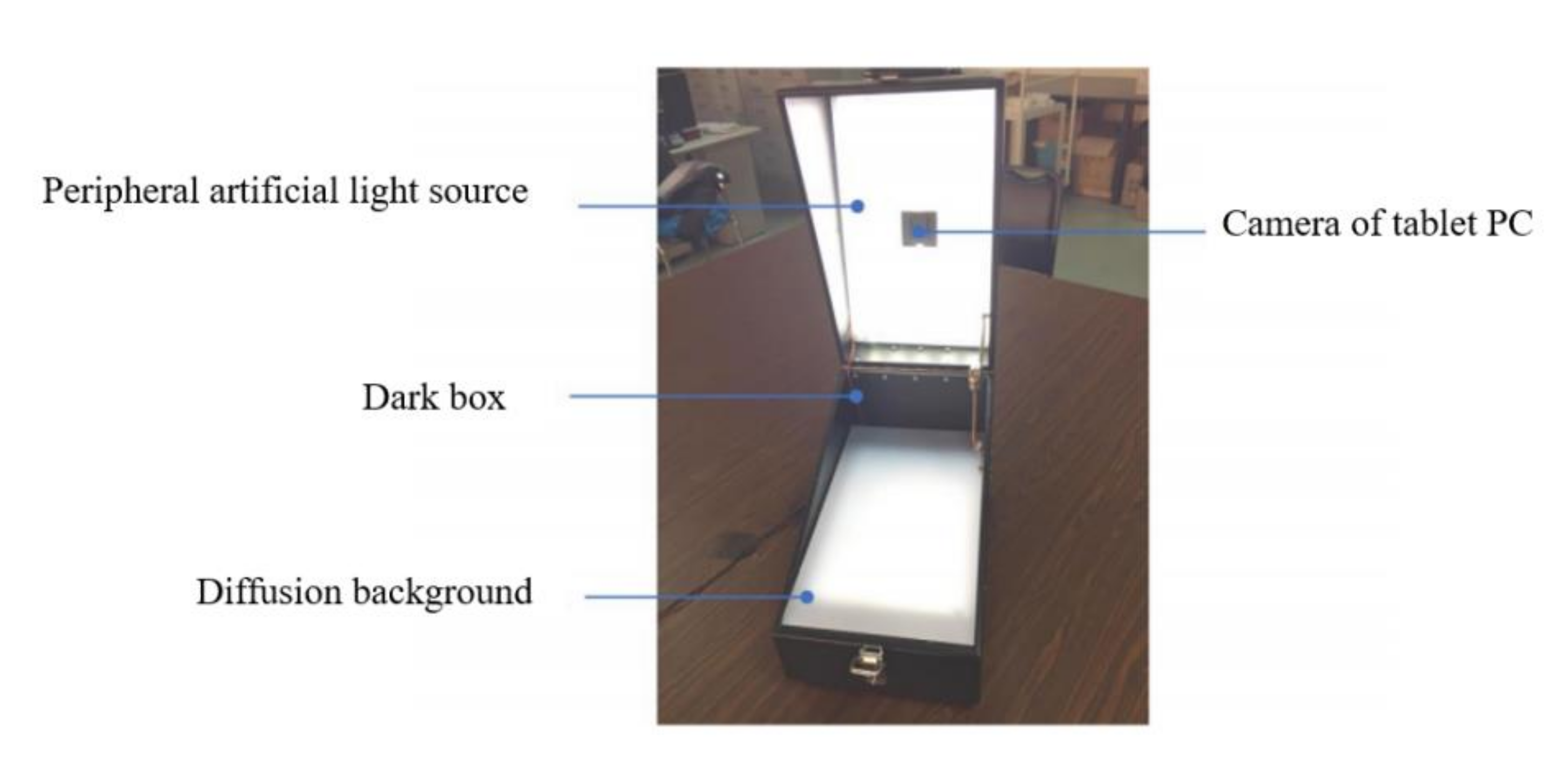
The portable phenotype platform consists of a dark box, a top LED strip, a top diffuser, a bottom diffuser, and a tablet PC, and its dimensions are 25 cm × 49 cm × 32 cm, as shown in Figure 1. The dark box is made of metal and connected by hinges. When using the dark box, you only need to open the dark box and put the leaves into the bottom diffuser, close the dark box, and use the tablet computer to take pictures. The top light source is composed of an LED strip plus a diffuser plate, which is used to simulate the surface light source. The top of the dark box has an opening for the tablet to take pictures, and the tablet is magnetically attached to the outside of the top of the dark box to take pictures of the plant leaves through the top opening. In addition, the top outer side of the dark box has a handle to make it easy for researchers to carry.
Considering the production cost of the portable image acquisition platform and the required performance, the Xiaomi Tablet 2® with a Cortex-A9 1.2G processor was chosen as the computation core in the instrument, with a camera resolution of 2048 × 1536 and autofocus support, which can largely meet the image acquisition needs. The tablet is powered by an Intel Atom x5-Z8500 quad-core processor, which can meet the computing requirements of the mobile recognition algorithm. In addition, the tablet runs on 2 GB of memory to meet the memory requirements of image processing algorithms.
2.2. Image Preprocessing
The background of the images collected by using the platform was white, because the background on the platform was white and a white light source was used. In addition, the degree of powdery mildew and leaf size of the collected cucumber leaves are varied. The background plate can transmit white light. Therefore, it can highlight the outline of the leaves in the picture for the convenience of leaf geometrics measurement during phenotyping. Since the main feature of the powdery mildew spots in the images is the white area, if the background is also white, it will have an impact on the recognition effect; therefore, in this section, based on these images, the white background in the images is transformed into a black background. The white powdery mildew spots are closer to the white background in the RGB color space, and direct background color conversion in the RGB color space may be unsuccessful, and it is easy to convert the white powdery mildew spots to black, as well. However, the HSV method can solve this problem. The image is first mapped from RGB space to HSV space, where H denotes the different color which is the color of the pixel point, S denotes the saturation of the color of the pixel point, and V denotes the brightness of the point. In general, the saturation component (S channel) can be used to distinguish between white backgrounds and white powdery spots. The transformation function is as follows:
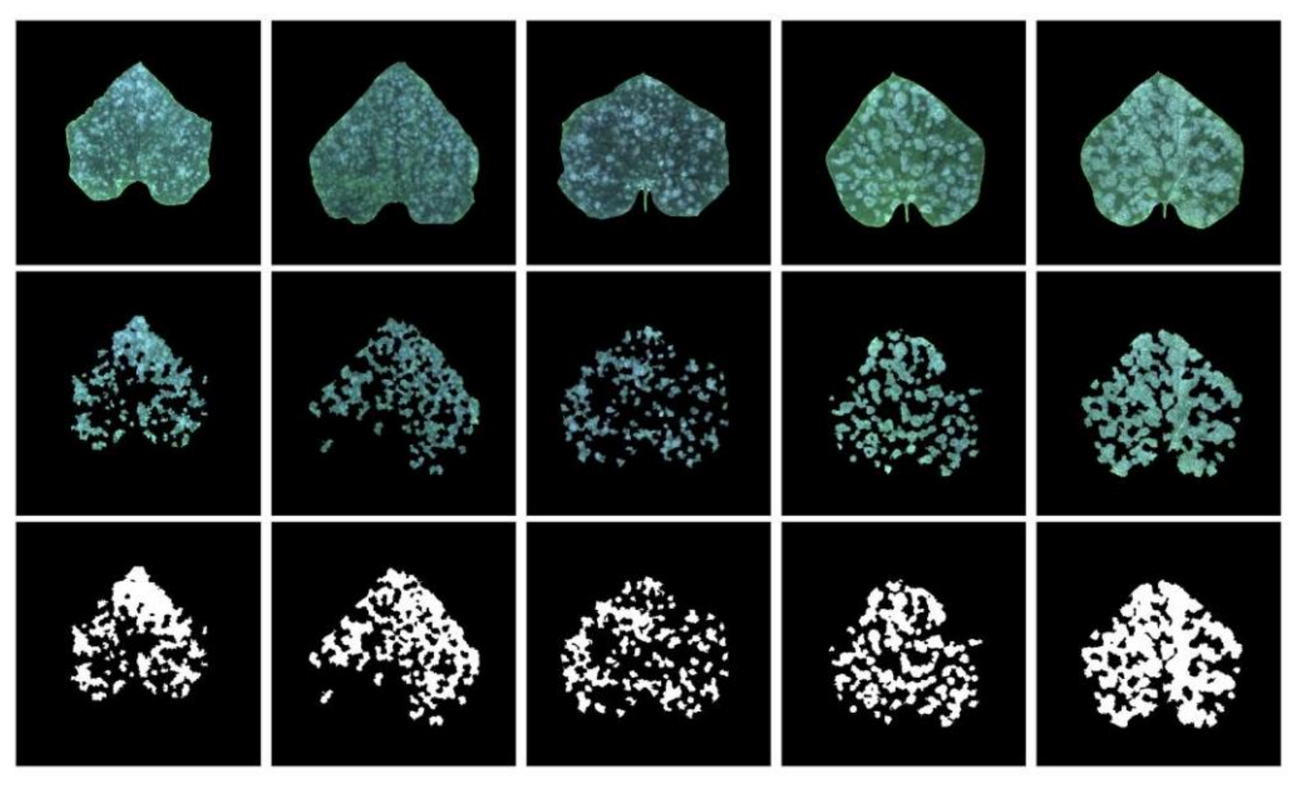
where p is the maximum of the three values of RGB at a pixel divided by 255, q is the minimum of the three values of RGB at a pixel divided by 255, and l = 1/2(p + q). After obtaining the background template in the S channel, the image with a black background is obtained by multiplying this template with each of the three RGB channels of the image. In addition, based on the empirical knowledge related to powdery mildew, the powdery mildew spot areas in each image were manually marked: the powdery mildew areas were marked as white and the non-powdery mildew areas were marked as black. The labeled images are shown in Figure 2.
2.3. Segmentation Model
2.3.1. Method of Simple Linear Iterative Clustering
Super-pixel, as the name suggests, is the aggregation of pixels in an image that have similar features in the same area, which can be texture, color, category, etc. Thus, these pixels can be treated as one pixel, which greatly reduces the number of pixel points and effectively reduces the computational effort during image processing. Considering that powdery mildew spots in images usually appear in blocks, pre-segmentation of images by using super-pixel methods can help improve the segmentation accuracy of powdery mildew spots.
Such segmentation algorithms are mainly divided into two categories: graph theory-based algorithms and gradient-based methods. The graph theory-based methods include the normalized cuts method [19], graph-based method [20] and optimal path method [21]. Gradient-based methods include Simple Linear Iterative Clustering (SLIC) [22], the Watershed approach [23], and the Turbopixel method [24].
Among them, SLIC is an efficient method for generating super-pixels by using K-means clustering. This method is characterized by its fast computation and low memory consumption. Therefore, this section uses the SLIC method to perform pre-segmentation operations on all pixels in an image.
Firstly, the number of super pixels (k) need to be set, and the image (CIELAB color space) is divided into grids with intervals of S pixels, so as to generate initial clustering centers Ci = [li, ai, bi, xi, yi]T (i = 1, 2, …, k). Each pixel should find the nearest cluster center with size S × S. Therefore, we should first search for similar pixels in the area 2S × 2S around the super pixel center to generate new cluster centers. Once the nearest cluster center of the pixel is found, the value of the cluster center is the average value of all pixels in the cluster. L2 norm is used to calculate the residual E between the new cluster center and the previous cluster center.
For two pixel points in a certain neighborhood, both the proximity of the two points in terms of distance and the similarity of the two points in terms of color are considered in the clustering process. In order to normalize these two types of metrics, the SLIC method uses a metric of normalized distance and color. The distance scale between two pixel points, pi and pj, is shown in Equation (2).
where l, a, and b are the values of the CIELAB color model of the pixel. Moreover, l represents luminosity, and the value range of l ranges from 0 (black) to 100 (white); a represents the range from magenta (127) to green (−128); and b represents the range from yellow (127) to blue (−128). Furthermore, x and y represent the coordinates of the pixel, dc represents the Euclidean distance between two pixel points in color space, ds represents the Euclidean distance between two pixel points in physical location, m is a customizable hyperparameter, and n is the Euclidean distance between starting points at grid division. The algorithm flow of the simple linear iterative clustering method is shown in Algorithm 1.
| Algorithm 1 Pseudocode of SLIC |
| Input: picture, Number of blocks k Process: 1: Initialize cluster center Ck by sampling pixels at regular grid steps S. 2: Move cluster centers to the lowest gradient position in a 2S × 2S neighborhood. 3: Set label l(i) = −1 and distance d(i) = ∞ for each pixel i. 4:do 5: for each cluster center Ck do 6: for each pixel i in a 2S × 2S region around Ck do 7: Using equation (2) to compute the distance D between Ck and i 8: if D < d(i) then 9: set d(i) = D, l(i) = k 10: end if 11: end for 12: end for 13: Compute new cluster centers 14: Compute residual error E 15: while E ≤ threshold Output: Image after super pixel segmentation |
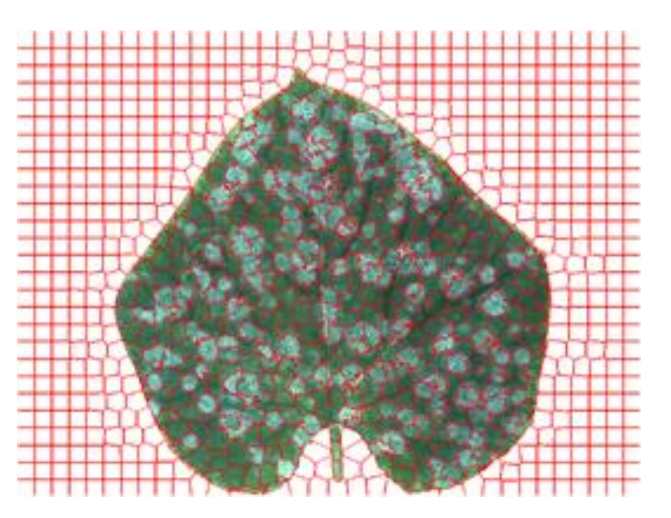
Figure 3 shows the effect of segmenting leaf image by using the SLIC method.
2.3.2. Hybrid Gaussian Model
In a plant-leaf powdery mildew image, pixels or super-pixels are divided into three main categories with their a priori semantics: the background, the healthy leaves, and powdery mildew spot areas. It stands to reason that the distribution of each class of pixels or super-pixels features in an image obeys a latent Gaussian distribution; then all the pixels or super-pixels in the whole image can be described by a Gaussian Mixed Model (GMM), with respect to unsettled parameters. Here, x is the characteristics value of a super-pixel block which is the mean value of all pixels in that super-pixel block in their respective color channels, i.e., the vector of the mean of all pixels in the R, G, and B channels. A multivariate Gaussian distribution probability density function can be represented by Equation (3).
where μ is the vector of the mean of the colors in three channels, ∑ is the vector of the covariance matrix. Then the probability density function of the GMM model is as follows:
where k is the number of Gaussian distributions, i.e., three types of super pixels (background, healthy leaves, and powdery mildew spots); μi represents the vector of the average value of the three colors of the ith super pixels; ∑i represents the covariance matrix of the colors of the ith super pixels; and αi is the mixing factor, a non-negative real number indicating the probability that the ith distribution is selected, i.e., the confidence that the super-pixel point belongs to one of the three types, where ∑αi = 1.
Since the generation of pixel points is assumed here to be given by a Gaussian mixing distribution, each sample generation process is as follows.
A certain Gaussian distribution is first picked according to the prior distribution defined by αk, and then the corresponding sample is sampled according to the probability density function of this Gaussian distribution. Let the random variable zj ∈ {1, 2, …, 𝑘} be the probability of the ith Gaussian distribution being picked. According to Bayes’ theorem, the posterior distribution of zj with respect to x is as follows:
Here, let γji = pM(zj = i|xj). xj is the new super-pixel, and pM (zj = i) is the confidence probability that the new super-pixel belongs to type i. Modeling the GMM model given the dataset D can be performed by using a great likelihood estimation method to maximize the likelihood function. The objective function is shown in Equation (6).
To maximize this function, the EM algorithm can be used to solve it. The parameters of the mixed Gaussian distribution (μ, ∑, and α) and the posterior distribution (zj) are estimated in the E step, using the parameters of the mixed Gaussian distribution (μ, ∑ and α) and using Equation (5) in the M step, using γji and combined with Equation (6), the parameters of the mixed Gaussian distribution can be calculated. The constant iterations of both can obtain the solution of the maximized likelihood function.
The posterior distribution of zj calculated in step E can be obtained according to equation (5), and the method of estimating the parameters of the mixed Gaussian distribution, using the posterior distribution in step M, is given below. In Equation (6), l(D) performs the partial derivative of μi and makes the partial derivative 0.
Similarly, find the partial derivatives for ∑i and αi, respectively, and let the partial derivatives be 0.
From this, a hybrid Gaussian model can be used to cluster the super-pixels in the image, thus realizing the need for disease spot segmentation. The algorithm flow is showen in Algorithm 2.
| Algorithm 2 Gaussian Mixture Model for superpixel clustering |
| Input: picture, Number of blocks k Preprocess: 0: use SLIC method to divide the image into xm super pixels, number of Gaussian distributions k = 3 Process: 1: Dataset D = {x1, …, xm}, randomly initialize μi, ∑i, αi 2: while 3: for j = 1, 2, …, m do 4: The posterior probability γji of each sample composition component is calculated according to Equation (5) 5: end for 6: for i = 1, 2, 3 do 7: Calculate the new μi, ∑i, αi according to Equation (8), Equation (9), and Equation (10) 8: end for 9: Update the parameters of the Gaussian Mixture Model to the new μi, ∑i, αi 10: do the parameter update difference is less than a threshold value 11: for j = 1, 2, …, m do 12: Find the category to which sample xji belongs according to argi max γji 13: Assign xj to the category to which it belongs 14: end for Output: Each super-pixel block belongs to a category {background, healthy leaf, powdery mildew spot}. |
The Gaussian Mixture Model can be used to model different types of pixel points and obtain the properties of each pixel point according to the distribution from which it comes, thus achieving the effect of image segmentation.
2.3.3. Lightweight Powdery-Mildew-Spot-Segmentation Model
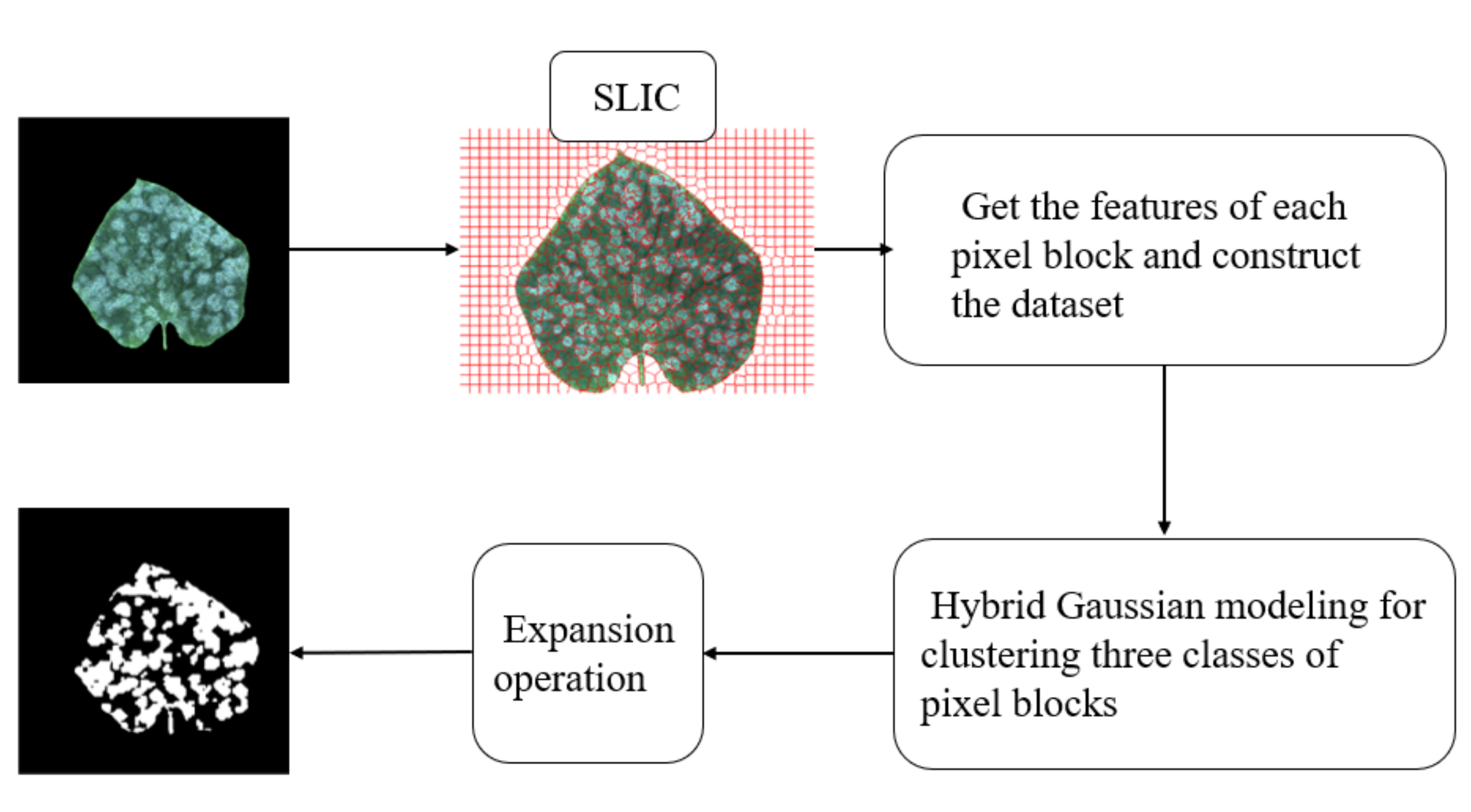
Based on the super-pixel segmentation method and hybrid Gaussian model, this paper proposes a lightweight powdery mild segmentation model. Firstly, we used the SLIC method to super-pixel segment the original image; secondly, we calculated the mean values of all pixels in each pixel block in the three RGB color channels and used them as features; subsequently, we used the hybrid Gaussian model to model the features of the three types of super-pixel points (background, healthy leaves, and powdery mildew spots) to obtain three Gaussian distributions. Then we took the distribution with the largest mean value as the distribution where the pixel points of powdery mildew spots are located. Finally, the posterior probability was used to find the pixel points belonging to the powdery mildew spots to construct the segmented image.
Considering the feature of under-segmentation by clustering method, we used expansion operation to alleviate the under-segmentation problem after obtaining the whitefly segmented image, using the hybrid Gaussian model.
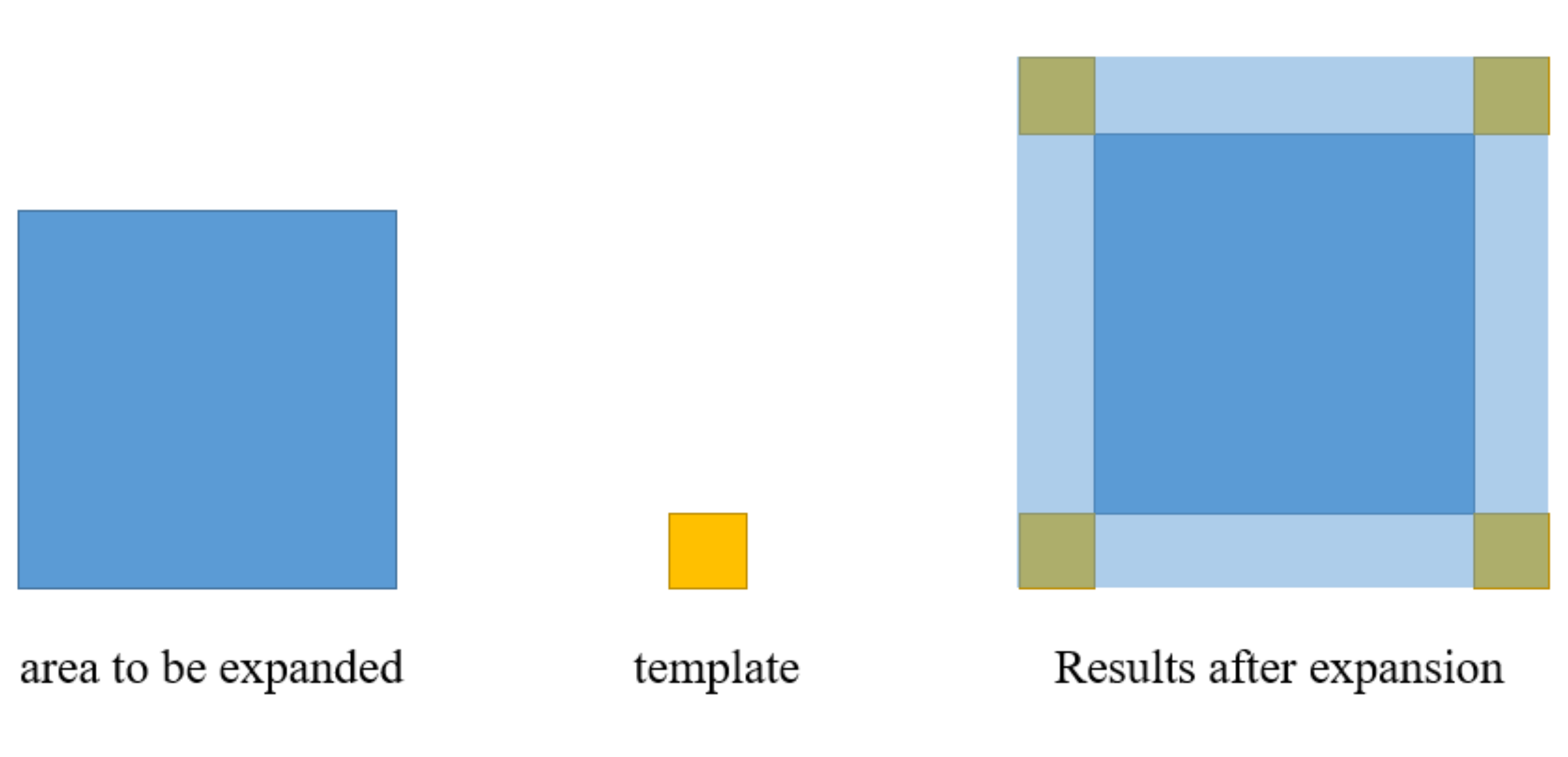
Generally, the expansion operation is performed on the image and is represented as follows:
where A is the original binary image, B is the template used for the expansion operation, and ()z indicates that the template B is translated by z units in A after performing the flip. The template is a solid square or circle with a reference point in the middle. The movement of the template in the picture is similar to the movement of the template in the picture in the convolution operation, thus allowing the current template centroid location to take a value of 1 when the intersection of the template and the original binary picture is not empty, as shown in Figure 4.
After the hybrid Gaussian model clustering, the image is inflated to finally obtain the whitefly spot segmentation image. The flowchart of the whole algorithm is shown in Figure 5.
2.4. Model Testing
In the experiment, we used six indexes to evaluate the performance of the model.
2.4.1. IoU Accuracy
The full name of the IoU is Intersection over Union, and it is specifically used to evaluate the performance of image segmentation methods. Its calculation formula can be expressed as follows:
where ptf denotes the area of the intersection of the real powdery mildew area in a picture and the area predicted as powdery mildew area by the model; and pt and pf denote the area of the real powdery mildew area in a picture and the area predicted as powdery mildew area by the model, respectively.
2.4.2. Dice Accuracy
The Dice is another metric to evaluate the performance of model image segmentation, and its value is usually larger than IoU for the same segmentation performance. Its calculation formula is as follows:
2.4.3. Pixel Accuracy
In simple terms, pixel accuracy is to consider image segmentation as a binary classification problem and get the classification of each pixel point and count it. The calculation formula is as follows:
Considering that the image segmentation problem can be essentially classified as a classification problem, the performance of the models is also evaluated by using Precision, Recall, and F-beta, so that the strengths and weaknesses of different models can be assessed from different perspectives. In this case, for the F-beta, the value of beta was chosen as 2 to give more weight to the recall. This is reasonable for plant-disease segmentation, since it is more important for disease identification not to miss disease regions.
2.5. Apps on the Instrumented Devices
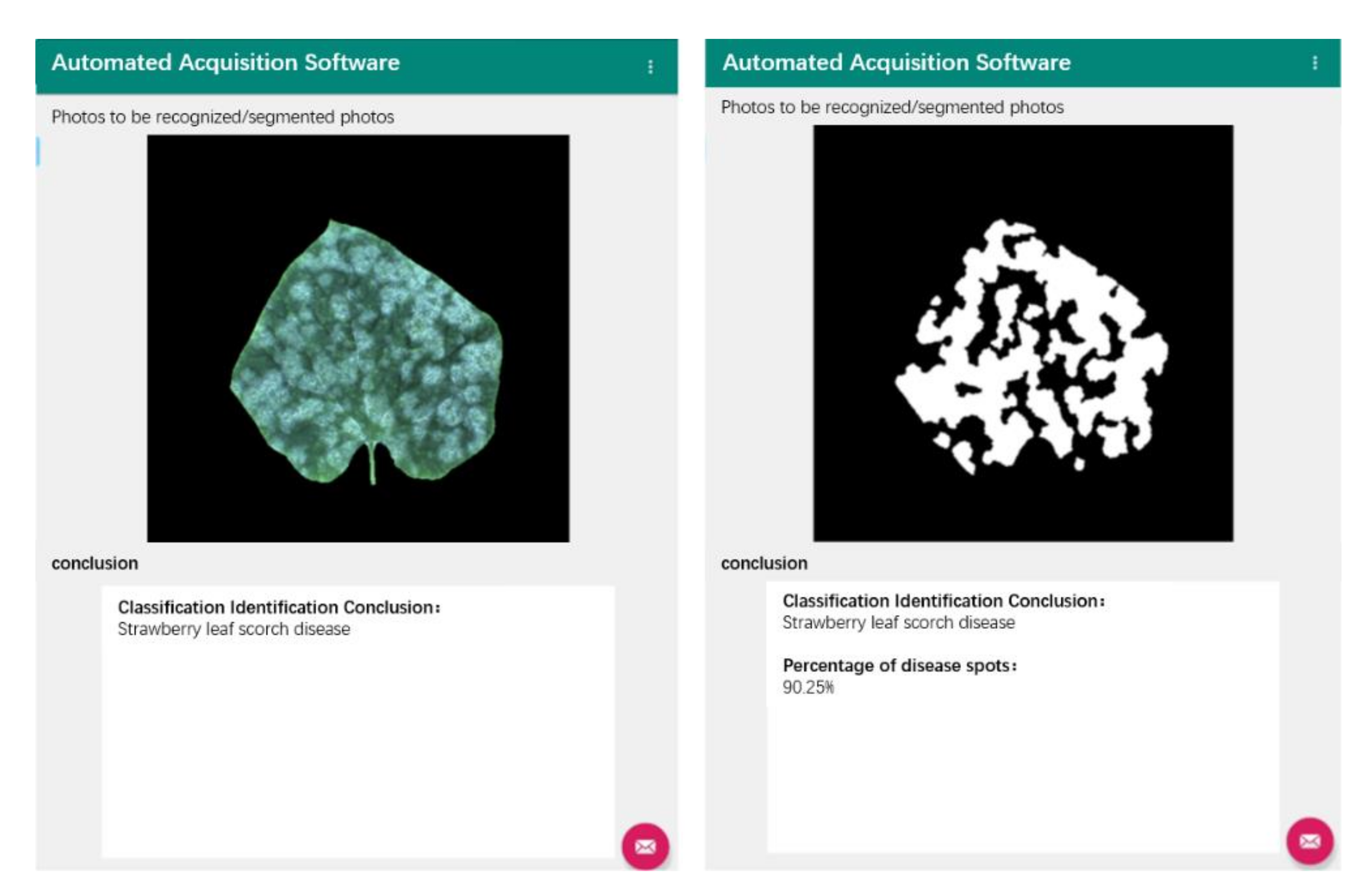
The automation recognition software was developed based on Android Studio and can run on Android phones or Android tablets, with a minimum adaptation to Android 4.0. The software’s whitefly spot recognition interface is shown in Figure 6. The upper part of the interface is the picture display area, the lower part is the conclusion display area, and the button in the lower right corner is used for some operations such as selecting pictures. In the recognition process, first select the picture; this step can be performed by directly opening the picture or calling the camera of the tablet computer to take the picture. After the picture selection is completed, click “start recognition” to get the recognition result. This software is able to perform pixel-level segmentation for powdery mildew spots, thus providing practitioners with the convenience of analyzing leaf traits quantitatively.
According to the runtime test, this method takes up the memory space, such as 3.6 M, for storing images in floating-point type, 12.8 M for the super-pixel segmentation part, 1.2 M for the Gaussian Mixture Model, and 163 M for the Python runtime environment, which runs in about 3s on a normal cell phone. However, the U-net model occupies about 2621 M of memory in CPU mode and cannot run in ordinary embedded devices or mobile devices. Therefore, this method meets the requirements of portable devices. If the method is rewritten in C, the memory consumption and running speed will be further improved.
3. Results
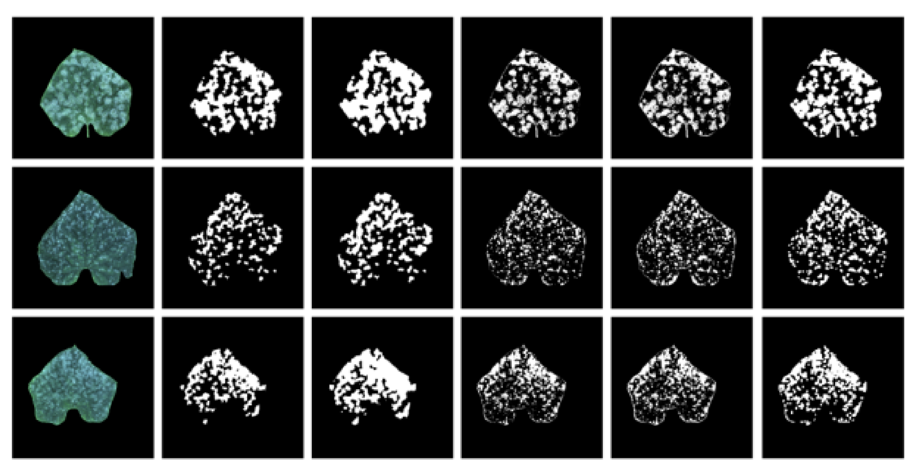
The segmentation effect of the proposed lightweight method in this paper is shown in Figure 7.
The first column is the original image, the second column is the manually labeled image, the third column is the result obtained by the U-net method, the fourth column is the segmentation result of the K-mean clustering method, the fifth column is the segmentation result of the maximum interclass variance, and the last column is the segmentation result of the method proposed in this paper. As can be seen from the figure, compared with other lightweight segmentation methods (K-mean clustering and maximum interclass variance), the present method solves the problem of under-segmentation of such methods to a certain extent.
Table 1 shows the detailed segmentation results of the proposed lightweight method on the test set in this paper, and it is worth stating that the method performs poorly in terms of accuracy on samples 1, 3 and 17, and better on the other samples. The lower accuracy on these two samples is the reason for the lower average accuracy. By analyzing the images of these three numbers, it was found that the diseased areas of these samples were smaller, and the clustering effect of the Gaussian Mixture Model became poor, resulting in some pixel points of healthy leaf areas being identified as powdery-mildew diseased areas, thus leading to lower recognition accuracy.
The average values of accuracy, recall, F2-score, IoU precision, Dice precision, and pixel precision are 65.94%, 82.35%, 76.52%, 57.80%, 71.38%, and 93.85%, respectively, among the 20 test samples, and the segmentation results meet the practical needs better. The results compared with lightweight methods, such as OTSU and K-mean clustering, and with convolutional neural networks, such as U-net, are shown in Table 2. Moreover, this method has significantly improved in the more important evaluation metrics, such as F2 score, IU precision, and Dice precision.
4. Discussion
In this paper, we proposed a lightweight powdery-mildew segmentation model. We firstly use a super-pixel segmentation method to pre-segment the images, secondly use a hybrid Gaussian model to model three classes of super-pixels (background, healthy leaves, and powdery mildew spots), and finally compensated for the spot areas by using an expansion operation and achieved powdery-mildew-spot recognition on a portable instrument for field use.
Compared to the clustering algorithmic counterparts, such as K-mean clustering and maximum interclass variance, the proposed method in this paper has better segmentation performance and achieves better results in both IoU metrics and Dice metrics. Meanwhile, when compared to such deep learning methods as the U-net, although the proposed method is slightly inferior to deep learning methods in terms of segmentation accuracy, its small memory consumption and low computational latency lend themselves to being deployed in embedded devices and smartphones to meet the needs of portable automated phenotyping. Compared with some lightweight neural networks, the proposed method does not require a large number of images for training the model to achieve high accuracy. In general, it lays a foundation for the portable automated phenotyping for powdery mildew disease in field detection and severity evaluation.
Author Contributions
Conceptualization, L.G., K.L. and C.L.; software, C.Y. and K.L.; validation, C.Y. and C.L.; formal analysis, L.G. and K.L. investigation, L.G. and K.L.; resources, L.G.; data curation, L.G., C.Y. and K.L.; writing—original draft preparation, L.G., C.Y. and K.L.; project administration, C.L.; funding acquisition, L.G. All authors have read and agreed to the published version of the manuscript.
Funding
This research was funded by Science and Technology Innovation Action Project of Shanghai Committee of Science and Technology, grant number 21N21900100; and the APC was funded by Shanghai Committee of Science and Technology, Shanghai, China.
Institutional Review Board Statement
Not applicable.
Informed Consent Statement
Not applicable.
Data Availability Statement
Data are available upon request from the corresponding authors.
Acknowledgments
The authors would like to thank Junsong Pan at School of Agriculture Science and Technology, Shanghai Jiao Tong University, for providing the powdery mildew leaves and image annotation.
Conflicts of Interest
The authors declare no conflict of interest.
References
- Sharma, P.; Berwal, Y.P.S.; Ghai, W. Performance analysis of deep learning CNN models for disease detection in plants using image segmentation. Inf. Processing Agric. 2019, 7, 566–574. [Google Scholar] [CrossRef]
- Mutka, A.M.; Bart, R.S. Image-based phenotyping of plant disease symptoms. Front. Plant Sci. 2015, 5, 734. [Google Scholar] [CrossRef] [PubMed] [Green Version]
- Wspanialy, P.; Moussa, M. Early powdery mildew detection system for application in greenhouse automation. Comput. Electron. Agr. 2016, 127, 487–494. [Google Scholar] [CrossRef]
- Zhang, S.; Wu, X.; You, Z.; Zhang, L. Leaf image based cucumber disease recognition using sparse representation classification. Comput. Electron. Agr. 2017, 134, 135–141. [Google Scholar] [CrossRef]
- Oppenheim, D.; Shani, G.; Erlich, O.; Tsror, L. Using deep learning for Image-Based potato tuber disease detection. Phytopathology 2019, 109, 1083–1087. [Google Scholar] [CrossRef]
- Mohanty, S.P.; Salathé, M.; Hughes, D.P. Using deep learning for image-based plant disease detection. Front. Plant Sci. 2016, 7, 1419. [Google Scholar] [CrossRef] [Green Version]
- Zhang, X.; Qiao, Y.; Meng, F.; Fan, C.; Zhang, M. Identification of maize leaf diseases using improved deep convolutional neural networks. IEEE Access 2018, 6, 30370–30377. [Google Scholar] [CrossRef]
- Khan, M.A.; Akram, T.; Sharif, M.; Awais, M.; Javed, K.; Ali, H.; Saba, T. CCDF: Automatic system for segmentation and recognition of fruit crops diseases based on correlation coefficient and deep CNN features. Comput. Electron. Agr. 2018, 155, 220–236. [Google Scholar] [CrossRef]
- Lin, K.; Gong, L.; Huang, Y.; Liu, C.; Pan, J. Deep learning-based segmentation and quantification of cucumber powdery mildew using convolutional neural network. Front. Plant Sci. 2019, 10, 155. [Google Scholar] [CrossRef] [Green Version]
- Zhang, S.W.; Shang, Y.J.; Wang, L. Plant disease recognition based on plant leaf image. J. Anim. Plant Sci. 2015, 25, 42–45. [Google Scholar]
- Ferentinos, K.P. Deep learning models for plant disease detection and diagnosis. Comput. Electron. Agr. 2018, 145, 311–318. [Google Scholar] [CrossRef]
- Zhang, S.; Wang, Z.; Wang, Z. Method for image segmentation of cucumber disease leaves based on multi-scale fusion convolutional neural networks. Trans. Chin. Soc. Agric. Eng. 2020, 36, 149–157. [Google Scholar]
- Hong, H.; Huang, F. Recognition Algorithm for Crop Disease based on Lightweight Neural Network. J. Shenyang Agric. Univ. 2021, 52, 239–245. [Google Scholar]
- Bi, P.; Luo, J.; Chen, W. Research on Lightweight Convolutional Neural Network Technology. Comput. Eng. Appl. 2019, 55, 25–35. [Google Scholar]
- Sandler, M.; Howard, A.; Zhu, M.; Zhmoginov, A.; Chen, L. MobileNetV2: Inverted residuals and linear bottlenecks. arXiv 2018, arXiv:1801.04381. [Google Scholar]
- Ma, N.; Zhang, X.; Zheng, H.; Sun, J. ShuffleNet v2: Practical Guidelines for Efficient CNN Architecture Design; Springer International Publishing: Cham, Switzerland, 2018; pp. 122–138. [Google Scholar]
- Wu, Y.; Xu, L. Lightweight compressed depth neural network for tomato disease diagnosis. In Proceedings of the Eleventh International Conference on Graphics and Image Processing, Washington, DC, USA, 3 January 2020; SPIE: Washington, DC, USA, 2020; Volume 11373, p. 113731S. [Google Scholar]
- Ji, M.; Zhang, K.; Wu, Q.; Deng, Z. Multi-label learning for crop leaf diseases recognition and severity estimation based on convolutional neural networks. Soft Comput. 2020, 24, 15327–15340. [Google Scholar] [CrossRef]
- Shi, J.B.; Malik, J. Normalized cuts and image segmentation. IEEE T. Pattern Anal. 2000, 22, 888–905. [Google Scholar]
- Felzenszwalb, P.F.; Huttenlocher, D.P. Efficient graph-based image segmentation. Int. J. Comput. Vis. 2004, 59, 167–181. [Google Scholar] [CrossRef]
- Moore, A.P.; Prince, S.; Warrell, J.; Mohammed, U.; Jones, G.; IEEE. Superpixel lattices. In Proceedings of the 2008 IEEE Conference on Computer Vision and Pattern Recognition, Anchorage, AK, USA, 23–28 June 2008; Volumes 1–12, p. 998. [Google Scholar]
- Achanta, R.; Shaji, A.; Smith, K.; Lucchi, A.; Fua, P.; Süsstrunk, S. SLIC superpixels compared to state-of-the-art superpixel methods. IEEE T. Pattern Anal. 2012, 34, 2274–2282. [Google Scholar] [CrossRef] [Green Version]
- Vincent, L.; Soille, P. Watersheds in digital spaces: An efficient algorithm based on immersion simulations. IEEE T. Pattern Anal. 1991, 13, 583–598. [Google Scholar] [CrossRef] [Green Version]
- Levinshtein, A.; Stere, A.; Kutulakos, K.N.; Fleet, D.J.; Dickinson, S.J.; Siddiqi, K. TurboPixels: Fast superpixels using geometric flows. IEEE T. Pattern Anal. 2009, 31, 2290–2297. [Google Scholar] [CrossRef] [PubMed] [Green Version]
Figure 1.
Main structure of portable plant-leaf automated phenotyping platform.

Figure 2.
Rows 1–3 are the raw images, their disease areas, and annotation of the areas, respectively.
Figure 2.
Rows 1–3 are the raw images, their disease areas, and annotation of the areas, respectively.

Figure 3.
Leaf image preprocessed by SLIC method.

Figure 4.
Expansion operation.

Figure 5.
Algorithm flowchart of lightweight segmentation model.

Figure 6.
Powdery-mildew recognition interface.

Figure 7.
Segmentation performance of different methods on three samples.


Table 1.
Segmentation results of the lightweight method on 20 test samples.
| No. | Accuracy | Recall Rate | F2 Score | IoU Accuracy | Dice Accuracy | Pixel Accuracy |
|---|---|---|---|---|---|---|
| 1 | 35.12% | 89.07% | 68.13% | 33.67% | 50.37% | 90.73% |
| 2 | 85.58% | 92.70% | 91.18% | 80.17% | 89.00% | 95.47% |
| 3 | 10.91% | 69.16% | 33.45% | 10.41% | 18.85% | 94.22% |
| 4 | 87.67% | 89.00% | 88.73% | 79.09% | 88.33% | 93.75% |
| 5 | 85.61% | 87.14% | 86.83% | 76.00% | 86.37% | 95.97% |
| 6 | 67.31% | 85.39% | 81.04% | 60.36% | 75.28% | 94.09% |
| 7 | 84.02% | 88.80% | 87.80% | 75.96% | 86.34% | 94.30% |
| 8 | 85.31% | 84.02% | 84.27% | 73.40% | 86.66% | 93.37% |
| 9 | 58.49% | 74.28% | 70.47% | 48.64% | 65.44% | 95.53% |
| 10 | 61.89% | 77.35% | 73.67% | 52.39% | 68.76% | 93.98% |
| 11 | 74.92% | 82.03% | 80.50% | 64.36% | 78.31% | 95.59% |
| 12 | 80.32% | 84.30% | 83.47% | 69.86% | 82.26% | 95.79% |
| 13 | 44.93% | 79.37% | 68.82% | 40.23% | 57.38% | 95.01% |
| 14 | 92.65% | 84.43% | 85.96% | 79.13% | 88.35% | 92.56% |
| 15 | 70.41% | 77.08% | 75.65% | 58.23% | 73.60% | 91.88% |
| 16 | 61.04% | 80.61% | 75.75% | 53.22% | 69.47% | 92.77% |
| 17 | 38.25% | 79.42% | 65.35% | 34.80% | 51.63% | 90.56% |
| 18 | 80.31% | 75.20% | 76.17% | 63.49% | 77.67% | 92.92% |
| 19 | 61.29% | 83.48% | 77.85% | 54.66% | 70.69% | 95.23% |
| 20 | 52.77% | 84.18% | 75.22% | 48.01% | 64.87% | 93.23% |
Table 2.
Results of lightweight methods on six evaluation indicators.
| Method | Accuracy | Recall Rate | F2 Score | IoU Accuracy | Dice Accuracy | Pixel Accuracy |
|---|---|---|---|---|---|---|
| Our method | 65.94% | 82.35% | 76.52% | 57.80% | 71.38% | 93.85% |
| OTSU | 69.39% | 58.78% | 59.20% | 45.33% | 61.48% | 92.04% |
| K-means Clustering | 71.35% | 60.55% | 60.83% | 47.05% | 63.11% | 92.33% |
| U-net | 73.30% | 97.34% | 91.20% | 72.11% | 83.45% | 96.08% |
Publisher’s Note: MDPI stays neutral with regard to jurisdictional claims in published maps and institutional affiliations. |
© 2021 by the authors. Licensee MDPI, Basel, Switzerland. This article is an open access article distributed under the terms and conditions of the Creative Commons Attribution (CC BY) license (https://creativecommons.org/licenses/by/4.0/).
Share and Cite
MDPI and ACS Style
Gong, L.; Yu, C.; Lin, K.; Liu, C. A Lightweight Powdery Mildew Disease Evaluation Model for Its In-Field Detection with Portable Instrumentation. Agronomy 2022, 12, 97. https://0-doi-org.brum.beds.ac.uk/10.3390/agronomy12010097
AMA Style
Gong L, Yu C, Lin K, Liu C. A Lightweight Powdery Mildew Disease Evaluation Model for Its In-Field Detection with Portable Instrumentation. Agronomy. 2022; 12(1):97. https://0-doi-org.brum.beds.ac.uk/10.3390/agronomy12010097
Chicago/Turabian StyleGong, Liang, Chenrui Yu, Ke Lin, and Chengliang Liu. 2022. "A Lightweight Powdery Mildew Disease Evaluation Model for Its In-Field Detection with Portable Instrumentation" Agronomy 12, no. 1: 97. https://0-doi-org.brum.beds.ac.uk/10.3390/agronomy12010097
Note that from the first issue of 2016, this journal uses article numbers instead of page numbers. See further details here.