1. Introduction
The degradation of land and ecosystem services caused by intensive tillage agricultural practices has prompted an alternative farming paradigm known as conservation agriculture [
1].
Conservation agriculture (CA) is an aggregate of best management practices that is built on three linked principles: minimum soil disturbance (i.e., no-tillage; No-T), preservation of a permanent soil organic cover, and crop rotation and diversification [
2]. These practices are meant to counteract soil degradation and enhance microbial biomass and water infiltration by minimum tillage. Meanwhile, mulching could diminish soil evaporation and runoff, enhance topsoil organic matter, and improve the stability of surface soil aggregates [
3,
4,
5,
6]. Moreover, No-T practices reduce production costs by decreasing fuel consumption and thus, greenhouse emissions [
1,
7].
Consequently, all these practices should sustain and increase crop productivity, and water and nutrient use efficiency, which would be translated into raising the farmer’s income. However, there is still the belief among farmers that CA practices can cause yield penalties, which is preventing their adoption and spread [
1,
8,
9]. Moreover, it is important to bear in mind that the benefits of CA previously stated may not be visible in the short term, but rather in the medium- and long-term results [
7,
9]. In addition, much research has been carried out about the effects derived from converting to CA, which highlighted diverse responses according to local characteristics. Thus, the overall outcomes demonstrated the need to design site-specific soil-management practices to translate their potential into environmental and economic benefits [
7].
The CA farming system has grown in recent years at a global scale, with CA cropland representing 12.5% of the total global cropland in 2016, with an increased tendency. Specifically, CA was implemented in 45% and 32% of the total cropland in USA and South America, respectively [
1]. In addition, although the Common Agricultural Policy of the European Union (CAP, Rural Development Programme 2014–2020) promoted the adoption of CA, there has not been a sustained and broad adoption of these practices in European agriculture, and CA farmland represents only 5% of the EU’s total cropland [
1]. Specifically, in the case of Italy, the part of arable land that farmers declared would be dedicated to No-T practices represent around 6% of the total Utilized Agricultural Area, according to the last available agriculture census [
10], which has been grant-supported by the rural development programmes of the Italian administrative regions [
11]. Therefore, these agricultural practices are still in a developing phase in Italy, with constraints for implementation in a lack of know-how and the mindset that CA would lead to yield penalties [
9].
The future CAP (2023–2027) has listed CA as an agricultural practice supported by the new so-called eco-scheme instrument, as these practices foster climate mitigation and prevent soil degradation. Therefore, farmers that promise to implement CA in their cultivation practices will be rewarded by this new instrument of the CAP policy [
12].
The durum-wheat crop cultivated in the Campania region represents 4.4% of the national surface (i.e., 1.21 million ha) and 4.5% of the national production (4.2 × 10
6 kg) [
10]. In the Campania territory there are three main milling industries, which represent 3% of the total national industries, with a producing capacity of more than 2 × 10
5 kg; and 15 pasta industries, which represent 13% of total national production. In Italy, semolina production reached 4.2 × 10
6 kg in 2020 (an increase of 9% compared to 2019) and 3.85 × 10
6 kg were used for pasta making [
13].
Italy is the second highest-producing country in the world of durum wheat (4.2 × 10
6 kg), after Canada (5.2 × 10
6 kg); and the first in Europe, which accounts for 49.4% (8.5 × 10
6 kg) of the total EU production [
14]. Among the Italian regions, Puglia (25.2% of the total national production) represents the top producer, reaching about one million tons, while Campania is listed in the eighth place [
10].
In the Campania region, the most common method for wheat cultivation is by conventional tillage (T), while direct seeding is barely spread and is decreasing [
9]. The impact of T is especially considerable in terms of energy and environmental factors in the hilly and mountainous areas of Campania because they predispose the land to water and wind erosion, that lead to a loss of fertility in cultivated land.
An increase in the severity and frequency of drought and floods events, changes in precipitation, temperature, and the carbon dioxide concentration in the atmosphere have been forecast for the Mediterranean region [
15,
16,
17]. This variability in the climate is predicted to have effects on soil water availability, carbon storage, and in crop yields and quality. Consequently, it is paramount to study farm management strategies that maintain agricultural production at environmental and economically viable levels. Among these strategies, CA is being fostered as valuable mitigation and adaptation practices to environmental changes that are affecting farming systems [
7,
18,
19]. Farmers have been able to adopt CA strategies in different agri-environmental characteristics to cope with climate variability [
20].
Field tillage experiments are time-consuming, expensive, laborious, and require specific expertise skills. Thus, properly calibrated crop process-based models may be used to evaluate the impact of diverse soil-management techniques on crop productivity and water–nutrients dynamics to identify the most appropriate and site-specific soil-management strategies [
1,
6,
21].
Some studies have employed crop-based models to evaluate the effects of different CA practices on crop performance, soil–water balance, and nutrients dynamics under different agro-environmental conditions [
19,
22,
23,
24]. However, these studies showed that most of the available crop models are not able to simulate accurately the long-term effects of the differences between CA and T [
25]. Authors argue that this fact may be due to missing specific modules (i.e., a tillage module) in the models to depict the effects of CA operations on soil variables [
4]; and flexibility in defining farm management practices that change season by season [
25].
Process-based crop modeling has been coupled with weather projections to gain knowledge on the effects of climate change on agricultural production, and thus identify the most appropriate CA strategies [
20]. In this way, crop modeling could provide insight on mitigations and adaptations to climate change by recognizing proper conservation agricultural practices [
26].
The ARMOSA model is a process-based cropping system model that has been proved to be suitable for field crops and to simulate different soil-management practices under diverse environmental conditions [
7,
27,
28].
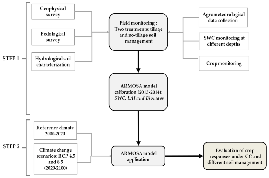
The overall objective of the study was to evaluate the effect of two different soil-management practices—T and No-T—on durum-wheat productivity and soil-related variables in the Mediterranean climate in current and future scenarios by using the ARMOSA model (
Figure 1).
The specific objectives consisted of (i) calibration of the parameters of the crop growth model for durum wheat under T and No-T soil-management techniques in a hilly Mediterranean region; and (ii) forecast wheat productivity, soil organic carbon (SOC) stock, and nitrogen (N) uptake under two contrasting climate-change scenarios for T and No-T soil management.
2. Materials and Methods
2.1. Site Description
The field data acquisition was conducted during the period 2013–2014 (October–June) in the durum-wheat field located in Scampitella (Campania, Italy 535 m a.s.l.). The durum-wheat field (Triticum durum Desf., var. Iride) covers 8.5 ha with a crop density of 350 viable seeds per m
−2. The selected farm is a representative durum-wheat farm in the Campania region in terms of farm size, economical dimensions, and agronomic and soil-management practices [
10].
The experimental area was located in two sites, with different soil-management strategies, which were used for field monitoring. The T treatment (1.5 ha; 41°08′77″N, 15°33′80″ E) involved ploughing in summer at 40 cm depth using a subsoiler, and in autumn at least two secondaries tillage using a disk harrow for seedbed preparation. The No-T management (No-T) (7.0 ha; 41°08′59″ N, 15°33′79″ E) started in the 2008–2009 growing season. A non-selective herbicide treatment was used (i.e., glyphosate at 3 L ha−1) for weed control, and after 7–10 days the durum wheat was sown with a specific seeder “Directa” 300 (:MASCHIO GASPARDO S.p.A., Campodarsego, PD, Italy) for undisturbed soil.
Before sowing and for both treatments, the basal fertilization was 36 kg N ha−1 and 42.24 P ha−1 (200 kg ha−1 of di-ammonium phosphate, DAP, 18-46-00), while during the initial tillering and stem-elongation stages of the durum wheat, 46 kg N ha−1 (100 kg ha−1 of urea 46-00-00) and 42 kg N ha−1 (200 kg ha−1 of sulfate of ammonia, SOA, 21-00-00) were applied, respectively. In both techniques, the management of crop residues was envisaged. The latter were chopped directly in the field by the combine harvester during harvesting (21 June 2014) and buried in the T treatment with ploughing and kept on the surface in the No-T treatment.
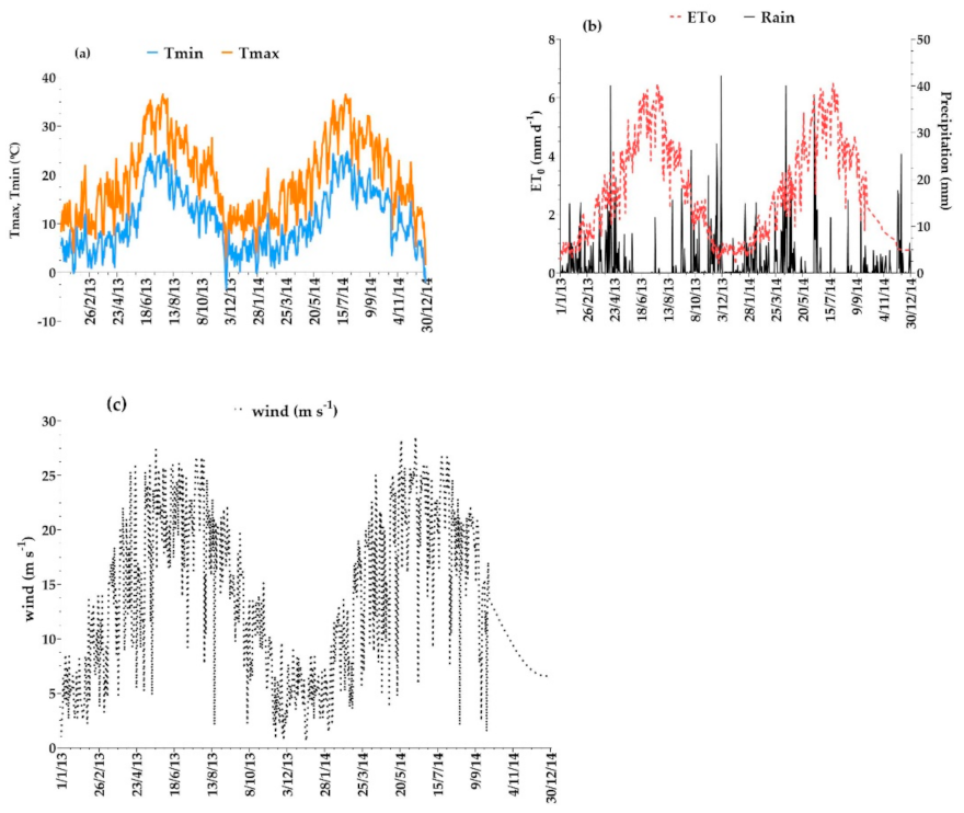
The climate is typically Mediterranean, with annual rainfall varying between 600 and 1000 mm, most of which falls in fall and winter; average monthly temperatures vary from 7 °C to 27 °C, respectively, from January to July (
Figure 2).
2.2. Soil Characterization
A geophysical scan of the farm soils using the electromagnetic induction (EMI) (GSSI: Nashua, NH, USA) sensor was performed to investigate the spatial variability of the field experimental farm. The EMI sensor allowed us to obtain aggregated information on the spatial variability of soils through the volumetric measure of the apparent electrical conductivity of soils.
The Profiler EMP-400 conductivity meter (GSSI: Nashua, NH, USA) was used to assess the soil’s apparent electrical conductivity. The Profiler used three frequencies at 5, 10, and 15 KHz in vertical dipole mode (VDM). The Tx and Rx coils were spaced 1.22 m apart with a depth of investigation of 1.95 m. The instrumentation was placed on a PVC sled and was towed by a tractor placed at about 5 m to avoid interference phenomena and data alteration. The use of the sled maintains a constant distance of the instrument from the ground to perform the acquisition faster and more easily.
The data obtained were filtered to eliminate any outliers, and then were subjected to variographic analysis and interpolated by ordinary kriging.
The pedogenetic horizons recognized in the opening of the soil profiles were sampled for the chemical–physical and hydrological analyses in the two plots located in the T and No-T field, respectively. Chemical analyses were conducted according to the Official Methods for Soil Chemical Analysis developed by the Italian Ministry of Agriculture and Forestry Policies [
30]. The soil organic matter was determined by oxidation with potassium dichromate solution in the presence of sulfuric acid following the Walkley–Black method. The pH values were determined in H
2O (soil/water suspension 1:2.5) and in KCl 1 M (soil suspension/solution 1:2.5). The CEC was determined according to the BaCl2 method at pH 8.2 and triethanolamine. The total carbonate content was determined by acid solubilization and gas-volumetric determination of CO
2, which takes place by treating a fine soil sample with hydrochloric acid and measures with the Dietrich–Fruehling calcimeter. The electrical conductivity was determined on aqueous extract, with water–soil ratio of 5:1.
The soil texture was measured by a laser diffractometry granulometer (Malvern Mastersizer 2000:Malvern, UK).
The hydraulic properties were carried out by laboratory analyses on undisturbed samples taken in each of the soil horizons. First, soil samples were saturated, then (i) the saturated soil water content, θs, was measured by a gravimetric method and (ii) the saturated hydraulic conductivity, ks, was measured using the falling head permeameter [
31].
Subsequently, after inserting three tensiometers at different depths in the soil sample, an automatically recording of the pressure head and the weight of the sample during a 1-dimensional evaporation process, allowed us to get three h(t) time series for the three different depths where the tensiometers were inserted and one averaged for the whole soil sample times series, θ(t) [
32]. From this information the water retention curve was obtained by applying an iterative method [
33]. Additional points of the dry branch of the water retention curve were determined using a dewpoint potentiometer (WP4-T, Decagon Devices, Washington, DC, USA). Finally, these water retention data were parameterized by fitting measured data to the van Genuchten model [
34].
2.3. Field Monitoring
The dates defining the crop phenological stages and the corresponding BBCH decimal code for the growth stages of durum wheat, following the Zadocks scale [
35], are indicated in
Table 1 for the crop-growing season of the study. The planting date of the two fields took place on 26 October 2013 using the Iride cultivar of durum wheat, and the harvest date took place on the 21 June 2014 in both fields (i.e., 236 days after sowing, DAS).
Table 2 illustrates the several variables measured in the experimental field.
A weather station (Watchdog 2900ET—Spectrum Technologies) was set up next to the experimental site for the hourly automatic acquisition of precipitation, air temperature at 2 m height, relative humidity, wind velocity, and solar radiation.
Plant biophysical characteristics (e.g., leaf area index, aboveground biomass) were measured starting from the tillering stage of wheat and up to harvest following the phenological stages indicated in
Table 1 to characterize the response of the plant to the two cultivation methods.
Eight aboveground biomass samples were taken from an area of 0.51 m2 (1.02 × 0.5 m), which included six contiguous rows. The sampling at harvest was taken from an area of 1 m2 within each test area and used to measure the following parameters: height of the plant (cm, excluding awns), total weight of biomass and grain (g m−2), and harvest index (weight of grain/total weight of biomass × 100).
The leaf area index (LAI) was measured by using LAI Licor 2000(LI-COR Inc.: Lincoln, NE, USA). Three random subareas of each experimental field were selected of 0.09 m2 (0.3 × 0.3 m), for a total number of nine samples in each field.
Once the LAI measurements were completed, the plant material collected was used for the estimation of the aboveground biomass (AGB) by drying in an oven at 65 °C until a constant weight was reached. Until 11 April, the plant material was mainly leaves. After this date, when stems and spikes were well-differentiated, the plant was separated into the different fractions. The total aboveground biomass was obtained by adding up the component fractions.
Rooting depth was measured on 7/2, 18/3 and 30/4/14 by trenching in the soil. Subsequent excavations did not show substantial differences compared to the observation on 30/4, therefore the measurements of the rooting depth were discontinued.
Three random test areas of 21 m2 each (7.0 × 3.0 m) were selected in each field to measure at harvest the grain yield (kg ha−1 adjusted to 13.0% moisture).
Two automatic stations were set up for data acquisition of soil water content by using the time domain reflectometry (TDR) technique. The stations adopted consisted of a Campbell TDR100 time domain reflectometer, to which are connected, through a system of SDMX50SP Campbell coaxial multiplexers, 12 probes.
The TDR probes were installed at 0–15, 20, 30, 40, and 50 cm depth according to the recognized pedological horizons. The probes were self-built and calibrated to determine the exact length of the cable and the electrical length, thus the probes were of the three-wire type with steel waveguides varying between 10 cm and 15 cm in length. The data acquisition and recording were carried out by a CR10X Campbell datalogger (Campbell Scientific: Logan, UT, USA). The waveforms were collected every 4 h starting from 18 November 2013 until 26 June 2014.
2.4. Climate Scenarios
Future climate scenarios were obtained by using the high-resolution regional climate model (RCM) COSMO-CLM [
36] employing a spatial resolution of about 11 Km at European level with optimization at Italian scale, able to employ a spatial resolution of 0.0715° (about 8 km). These last model data were validated, resulting in agreement with different regional high-resolution observational datasets, in terms of average temperature and precipitation [
37] and in terms of extreme events [
38].
In particular, two different simulations were performed by employing two standard IPCC (Intergovernmental Panel on Climate Change) RCP4.5 and RCP8.5 greenhouse gas (GHG) concentrations [
39]. Specifically, the RCP4.5 scenario shows stabilization in the GHG emissions, while the RCP8.5 scenario has a rapid increase of the GHG concentration. The initial and boundary conditions for running RCM simulations with COSMO-CLM were provided by the general circulation model CMCC-CM [
40], whose atmospheric component (ECHAM5) has a horizontal resolution of about 85 km. For both future climate scenarios, the period considered in the simulation was 2020 to 2100 and the solar global radiation was calculated using the RadEst 3.00 software (FAO, ISCI: Rome, Italy) [
41]. Specifically, the Campbell/Donatelli radiation model implemented in RadEst was used.
Observed weather data over the period 2000–2020, provided by the Protezione Civile della Regione Campania
http://centrofunzionale.regione.campania.it/ (accessed on 20 Semptember 2021) was used as reference climate to check the climate scenario forecast. For that period, the annual mean rainfall was about 829 mm and the mean air temperature was about 13.4 °C, with reference to the Ariano Irpino site (Campania region, Italy), which is at 28 km distance from the experimental site and at the same elevation.
2.5. ARMOSA Model
Model Description
The ARMOSA model simulates soil- and crop-related variables in response to agricultural management and pedoclimatic conditions. The model runs at a daily time step and consists in three main modules: (1) crop growth and development; (2) soil water dynamics; (3) C and N cycling.
The crop-growth simulation was based on the gross C absorption following the WOFOST approach [
42] with a substantial improvement: the canopy was divided into five layers with different light interception. For each crop, 65 parameters needed to be set. During previous model applications [
43,
44,
45], most of these parameters’ values had been set. In the present study, the most sensitive parameters (i.e., potential gross C adsorption, specific leaf area index (LAI), four cardinal temperatures for crop growth) were set using the measured data from the field experiment with an objective function based on yield and LAI. As for the crop development, the model calculates the growing degree days (GDD), the development rate (used in the assimilate partition and LAI estimation), and the vernalization factor. BBCH scale is used to indicate the crop stages. In this analysis, the GDD requirements and the base temperature, optimal minimum and maximum temperature, and cut-off temperature for each stage were defined based on the observed dates of the durum wheat. The crop development is based on GDD, which were calculated by applying a trapezoidal rule that is similar to the rule described by [
46]. Photosynthates partitioning among plant organs is specific for each BBCH stage.
Water content was simulated for each soil layer by a daily bucket module where the soil profile is divided into layers, usually 5 cm thick. Each layer accumulates water until it reaches the field capacity; above this level, the model tries to transfer the water in excess to the layer below within the limit of the hydraulic conductivity. The water that cannot infiltrate the lower layer (because it exceeds the hydraulic conductivity, or the lower layers is already at saturation) is retained up to the saturation level. The water that tries to infiltrate from the top into a layer that is already at saturation point bounces back and (proceeding from the bottom to the top of the profile) can remain above the soil surface for the rest of the day. This module calculated the daily soil water content in each 5-cm layer as the results of the water input (rain and irrigation), water uptake by roots, and percolation. The simulation was strictly dependent on soil properties.
C- and N-related processes were simulated for each soil layer and implemented following the approach of the SOILN model [
47], with the difference that each input of C and N was considered independently, with each one having its own decomposition rate and fate. The input could be of three types, to which correspond three types of organic C and N pools: stable, litter, and manure. Crop residues, being the input of the litter pool, decompose based on the tillage type, depth of soil incorporation, crop type, and organs. Mineral pools are carbon dioxide, ammonium, and nitrate. Mineral and organic pools were daily calculated for each layer as the results of soil processes, which are immobilization, mineralization of the organic pools C and N, nitrification, crop uptake, nitrate leaching, denitrification, atmospheric deposition, ammonium volatilization, and nitrous oxide emissions. The processes were driven by the temperature and water level, which affected the microbial activity. The inputs were manure (e.g., dairy or swine slurry, dairy dung, digestate, sewage sludge) or litter (i.e., crop residues or green manure). The soil temperature was simulated according to [
48,
49] (SWAT model); it was mainly driven by crop biomass, litter, the stable fraction of SOC, and SWC.
The model input requirements in the current study considered the following data:
(a) Soil data: soil properties (i.e., sand—%, silt—%, clay—%, bulk density—Mg m−3, SOC and N in stable, litter, and manure fractions—kg ha−1, van Genuchten–Mualem equation parameters) are required for each pedological horizon. The horizons were further split into 5-cm layers for the daily estimation of the soil-related variables. In each layer, the state variables were water availability and percolation, evaporation, soil organic C and N in the three main pools (i.e., stable, litter, manure), ammonia, and nitrate. ARMOSA computed the daily values of bulk density and van Genuchten–Mualem equation parameters as affected by SOC content and tillage operations.
(b) Daily weather parameters were required as input data to compute the reference evapotranspiration (mm d
−1) with the Hargreaves-reference evapotranspiration equation [
29]. The required parameters were rainfall (mm), minimum and maximum air temperature (°C), wind speed at 2 m height (m s
−1), and solar global radiation (MJ m
−2).
(c) Crop data: the crop rotation had to be set and for each crop sown and harvested, dates had to be entered. The input for crop-residues management was the percentage of residues biomass retained and the soil depth of incorporation.
(d) Tillage date, type (perturbation and mixing effect), and soil depth had to be defined for each tillage event.
(e) Fertilization: either mineral or organic fertilizers had possibly been applied. The amount of kg N ha−1, day of the year (DOY) of application, depth of application, the type of fertilizer (ammonium and nitrate content, C/N ratio for organic fertilizers) had to be set.
2.6. Model Parametrization and Calibration
The model was calibrated for the prediction of the soil water content (SWC), leaf area index (LAI), and the aboveground biomass (AGB) collected in the two experimental sites located in Scampitella (South of Italy). Therefore, the ARMOSA model was calibrated using the set of measured data collected on the tillage (T) treatment and on the no-tillage (No-T) treatment of the durum-wheat-cropping system during the 2013–2014 crop growing season.
The calibration methodology followed a trial-and-error procedure to minimize, with an iterative process, the error propagation in the simulated processes, as described in [
50]. The trial-and-error procedure consisted, first, of finding the soil hydraulic parameters in the T and No-T management treatments for the different soil depths, until the variation of the differences in SWC sim—SWC field became negligible with few deviations from one iteration to the successive. This calibration of hydraulic properties was required for field applications to consider the well-known deviation between laboratory-measured and field-measured hydraulic properties [
51,
52,
53].
Secondly, the same method was developed for the crop phenological stages and crop parameters in the T and No-T treatments, until low estimation errors were obtained, with negligible differences in successive iterations for the phenological dates, LAI, and AGB field data. Therefore, the same values of the crop calibrated parameters were used in the T and No-T treatments.
The performance of the model was assessed graphically and using the following goodness-of-fit indicators, which were employed and suggested in former modeling studies [
27,
50,
54].
For all the indexes, Oi and Pi relate to observed and predicted values for all studied variables and and are the mean of the observed and predicted variables, respectively.
- (a)
the Pearson’s correlation coefficient (
r) [
55] is a measure of the degree of association between simulations and observations. It varies between 0—no agreement and 1—full agreement between the simulated and observed data:
- (b)
the relative root mean square error (RRMSE) [
56] is a measure for the accuracy of the predictions, which needs to be equal or close to 0, evidencing a perfect match between the simulated and observed variables.
- (c)
the average absolute error (AAE) represents the average error size associated with the estimations, and it varies between 0—perfect match and positive infinitive—no match between the simulated and measured values:
- (d)
the percent bias (PBIAS) [
57] indicates the trend of the model predictions to be larger or smaller than the equivalent observed: positive values indicate an underestimation bias, while negative values correspond to an overestimation bias and values close to zero indicate the absence of trends:
- (e)
the efficiency index (EF) proposed by [
58] varies between negative infinity and 1.0, whose positive values indicates that the model is a better forecast than the average of measured values:
The calibrated model was run with the two climate scenarios RCP4.5 and RCP8.5, and the crop phenological stages were modified according to the climate trend observed (i.e., higher temperatures and lower rainfall events). Previous research predicted an elongation of the crop-growing season in future periods, and thus the model needs to be modified accordingly for future scenarios [
18,
59].
As a matter of fact, in this study, the sowing and harvesting dates were kept the same as those observed in the monitoring year. The flowering stage was anticipated and the time for grain maturity reduced to elongate the wheat growth cycle by adjusting the thermal requirements in growing-degree days from the tillering to the flowering stage and from watery ripeness to physiological maturity.
The following output parameters were analyzed in the model application: predicted grain yields, SOC content, N uptake, and water- and nitrogen-stress indexes; to verify their long-term trends and stabilities under the two soil-management techniques.
The one-way ANOVA model was applied to data, considering annual results as replicates, to find differences between T and No-T, and the homogeneity of variances was tested using Levene’s mean-based test [
60] following the suggestions of [
61].
3. Results
3.1. Soil Survey Results and Plot Definition
A preliminary scan of the two fields was performed by EMI sensors to investigate the soil variability in both fields and, thus, define the experimental plots.
Most of the area—excluding some spots—showed similar values of ECa between the range 60–80 ms cm
−1. This homogeneous response of the soil profile cannot be directly reflected in a soil homogeneity, because the ECa is an integrated value that depends on many factors such as soil texture, layering, water content, and salinity—different combinations of which can produce similar results. Therefore, two profiles were open in zones showing the same value of ECa, respectively in the T and No-T field (black circles in the
Figure 3), on the base of this first hypothesis on homogeneity.
Both soil profiles are Calcic Vertisols according to the World Reference Base (WRB) classification system [
62]. In
Table 3 the main characteristics of the soil profiles are reported. Only minor differences arose between the two profiles in genetic horizons, pH, carbonates, and CEC. Hence, the possible differences in the results obtained in the two experimental plots cannot be attributed to differences in soils but—reasonably—only to the different tillage of the upper layer, i.e., conventional and no-tillage.
According to these preliminary results, the experimental plots of T and No-T were selected near to the profiles, and their location is reported in
Figure 3 with a black circle.
3.2. Parameter’s Calibration of the Durum Wheat Crop Growth Model
The ARMOSA model was calibrated using SWC measurements, LAI, and AGB in both T and No-T treatments for the entire crop-growing season.
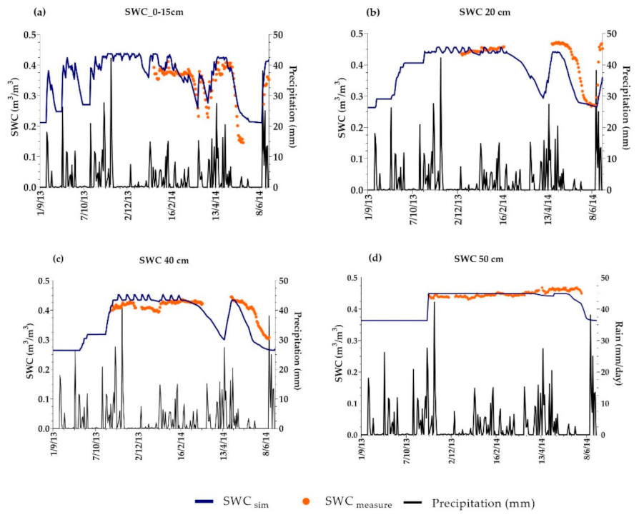
Figure 4 shows the match between measured and simulated SWC values during the crop-growing season 2013–2014 at 0–15-cm (n = 123), 20-cm (n = 133), 40-cm (n = 194), and 50-cm (n = 194) depths regarding the T treatment. The results show that the temporal variations of both measured SWC and estimated SWC are reasonably well-described for the whole period and for the four depths. Moreover, the model responded well to the peaks and absence of rainfall events.
The calibration indicators for the four soil depths and the entire soil profile are reported in
Table 4. Overall, the goodness-of-fit indicators performed well for the four soil depths and along the soil profile, with slight differences between the more superficial and the deepest soil layer. The Pearson’s correlation coefficient r values were high in the 0–15-cm, 20-cm, and 50-cm depths (r = 0.91–0.88) and acceptable in the 40-cm depth (r = 0.51), which indicates that the model represented with good accuracy the variability of the SWC in each layer.
The model underestimates the SWC at 20 cm with a PBIAS of 13.1%, while smaller PBIAS values (0.6–2.4%) were found in the other depths with no trend of under- or over- estimation of the simulated values. Estimation errors are small in all depths, as indicated by the RRMSE < 16% and AAE < 0.05 m3 m−3. The Nash and Sutcliffe efficiency index EF was high for the superficial layer (EF = 0.79), acceptable in the 20-cm layer (EF = 0.23), and negative for the deepest layers (EF = −0.05; −0.43), which means that the mean square error was higher than the measured data variability.
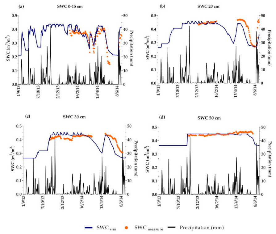
As in the T treatment, calibration results showed good agreement between simulated and measured SWC data at 0–15-cm (n = 125); 20-cm (n = 128), 30-cm (n = 169), and 50-cm (n = 186) depths for the No-T treatment. The simulated SWC followed the temporal SWC measured (
Figure 5), and the statistical indicators depict similar ranges as the ones for the T treatment (
Table 4).
The r coefficient was near to 1.0 in the more superficial depths, which indicates a good linear correlation between the simulated and measured data sets in the first three depths investigated (r = 0.83–0.79). Contrarily to that observed in the T treatment, the r index at 50 cm is lower than those in the upper layers. The PBIAS results were acceptable and did not perform any significant over- or underestimation trend of the model output in any of the soil layers. Estimation errors RRMSE and AAE were in the same range as the ones in the T treatment for each soil layer investigated.
In the same line, the EF index performed similar values that those in the T treatment output, which depicted satisfactory EF in the upper layers (EF = 0.55–0.32) and negative value in the lower layers (EF = −0.47;−1.15).
Measurements of LAI and AGB for the whole crop-growing season in the T and No-T management methods were used for further calibration of ARMOSA.
Figure 6 represents simulated LAI and AGB obtained with the calibrated model parameters compared with the measured LAI
measure and AGB
measure data, and
Table 5 reports the statistical indices outcomes from the model calibration. The results illustrate that the simulated LAI and AGB adequately fits the measured variables.
The model calibration indices (
Table 5) are acceptable for LAI and good for AGB predicted values. In both treatments, the Pearson’s correlation coefficient r is high (0.98–0.84) for LAI and AGB, which reflects high correlation of the simulated and measured variables. In the same way, the estimation errors RRMSE and AAE are acceptable for the LAI and small for the AGB variable.
The PBIAS is small for the AGB variable and LAI in the No-T but indicates an overestimation by the model of the LAI measured values (−18.2%) in the T treatment. This may be related to the fact that the LAI measured values in the No-T management were 1.25–1.50 times higher than the ones in the T management, which may cause the overestimation of the LAI in the No-T management.
Similarly, the EF index regarding the LAI calibration in the T is negative (−0.73), which could be due to the small difference between the minimum and maximum measured values of LAI. The predicted values could not simulate the small range of measured values, but the simulated curve fitted the pattern of the measured values.
On the other hand, the EF index of the AGB prediction is high (EF = 0.93–0.91), which shows that the simulations of AGB have a small error with respect to the variance of observations.
According to this statistical evaluation, the calibration of ARMOSA for durum wheat cultivated with T and No-T was performed satisfactorily, even better than similar experiments [
3,
4,
21].
3.3. Simulations with Climate-Change Scenarios
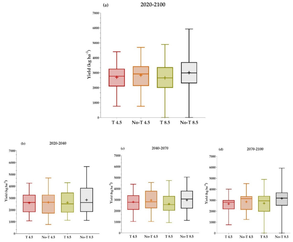
The simulation results obtained by the ARMOSA model for the two climate scenarios during the 2020–2100 period, three timeframes (2020–2040, 2040–2070, 2070–2100), and the two soil-management treatments are presented in
Figure 7 as box-plot graphs. The average yields of the No-T treatment are 5.2% and 11.4% higher than the T treatment yield in the 4.5 and 8.5 climate-change scenarios, respectively, when considering the period 2020–2100. The difference of the average yield between the two soil-management techniques is not statistically significant (
p > 0.05) in the RCP4.5 scenario but is statistically significant in the RCP8.5 scenario (
p < 0.05).
The yield difference between the two soil-management treatments becomes more pronounced as time advances, and is always higher in the No-T treatment. For instance, yield difference reaches the minimum in the two scenarios during the 2020–2040 timeframe (0.37% and 4.12% in the 4.5 and 8.5 RCP scenarios, respectively), and it will be maximum during 2040–2070 in the RCP8.5 scenario (15%) and in 2070–2100 considering the RCP4.5 scenario (12%).
It could be observed from
Figure 7 that the yield variability is slightly higher in the No-T management in comparison to the T in both scenarios and for each timeframe considered. However, this difference is not statistically significant (
p > 0.05) in any case considered, as shown by the Levene test. In addition, the largest variability of the average yield is observed in the RCP8.5 scenario in both soil-management techniques.
The evolution of the total SOC in the first 30 cm of soil along the future period for both climate scenarios (
Figure 8) is improved when the No-T treatment is implemented in durum wheat in this pedoclimatic context. The SOC content remains constant during the first years of implementation of the No-T management, then starts to increment constantly with an average annual growth rate of 0.19% year
−1 in the RCP4.5 scenario and 0.20% year
−1 in the RCP8.5 scenario, until it reaches a constant value. On the contrary, the use of T management in durum wheat will produce a constant reduction of the soil carbon content with an average annual growth rate of −1.32% year
−1 in the RCP4.5 scenario and −1.35% year
−1 in the RCP8.5 scenario, until it reaches a minimum value around 10,000 kg ha
−1 SOC.
As a matter of testing, we calculated the relationship of the SOC in both treatments, I
SOC = SOC
T/SOC
No-T, as measured at the beginning of the experiment in 2013, measured after 8 years in 2021, and modeled for both RCP scenarios for 2013 and 2021. The results are reported in
Table 6.
Consequently, the different trends in the SOC in the two soil-management systems of durum wheat under these pedoclimatic conditions can be predicted by the ARMOSA model for future climate projections.
The N uptake will be much higher when the No-T technique is used, depicting an annual average change of 3.55% year
−1 in the RCP4.5 scenario and 3.18% year
−1 in the RCP8.5 scenario, which at the same time will reduce the N leaching (
Figure 9). The No-T system will not experience N stress, although the uptake is higher in this management (
Table 7). On the other hand, the system under T will not absorb as much N as the No-T, depicting 1.57% year
−1 and 1.73% year
−1 of average annual change, respectively for the RCP4.5 and RCP8.5 scenarios; and thus, it won’t be able to produce much more yield, as explained previously.
Table 7 shows the N and water stresses that the crop system will experience in the future period. Neither technique will give any important stress. The difference in water stress between the two techniques will be small, although there may be more stress in the No-T treatment because the crop system will produce more, and, thus, consume more water. The residues kept in the soil decrease the evaporation process and the crop may be able to use water more efficiently, which may lead to a higher water consumption, and, thus, a slightly higher water-stress index.
5. Conclusions
The ARMOSA model was effectively calibrated for the durum-wheat crop system grown under tillage and no-tillage techniques in the Campania region, using SWC data, LAI, and AGB measurements. Estimation errors were small, with RRMSE averaging 10.67% for SWC at different depths, 26% for LAI, and 16% for AGB simulations. In addition, the model was further applied for the T and No-T management methods using the RCP4.5 and RCP8.5 climate-change scenarios. These simulations depicted the importance of implementing No-T management in durum-wheat cultivation to counteract climate change. The No-T will maintain higher yields than the T technique, will preserve and improve SOC along the years, and enhance the N uptake, thus diminishing N leaching.
Therefore, these results suggest the appropriateness of ARMOSA model to quantify the effects of different soil-management techniques on soil-crop related variables of durum wheat system under current and future climate.
Further studies are suggested to include the three principles of CA in the model simulations—for instance, diverse crop sequences and associations, permanent soil cover, and minimum soil disturbance. The potential role of adopting simultaneously these principles is crucial to achieve C sequestration, and to improve soil moisture and nutrient availability, among other matters.
However, the most suitable soil-management techniques are site-specific to achieve more benefits. In this sense, simulation models such as ARMOSA are important instruments to assist decision-making in a certain context to assess the effectiveness of soil-management techniques prior to their implementation, also in the view of future climate change.


 ,
, 


