
A Simple and Accurate Method Based on a Water-Consumption Model for Phenotyping Soybean Genotypes under Hydric Deficit Conditions

 and
and 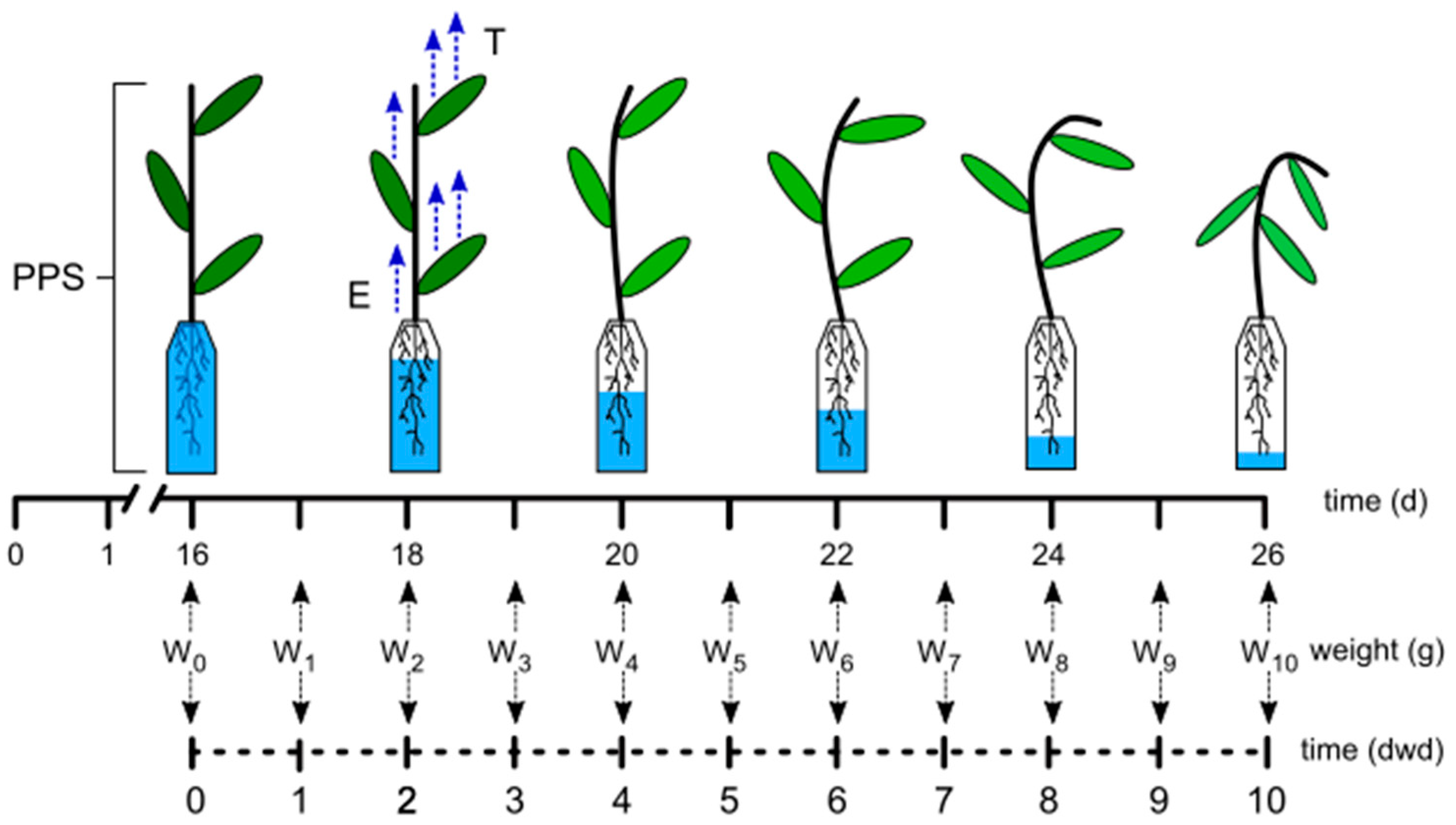
Abstract
:1. Introduction
2. Materials and Methods
2.1. Phenotyping Method Based on Water Consumption under Controlled Environmental Conditions
2.2. Phenotyping Strategy Applied to an F3 Segregating Population
2.3. Phenotyping Strategy Applied to a Breeding Population
2.4. Genotyping by Sequencing and SNP Calling
2.5. Data Analysis
2.5.1. Nonlinear Models
2.5.2. Multivariate Characterization
2.5.3. Statistical Model and Adjustment of Phenotypic Means
3. Results
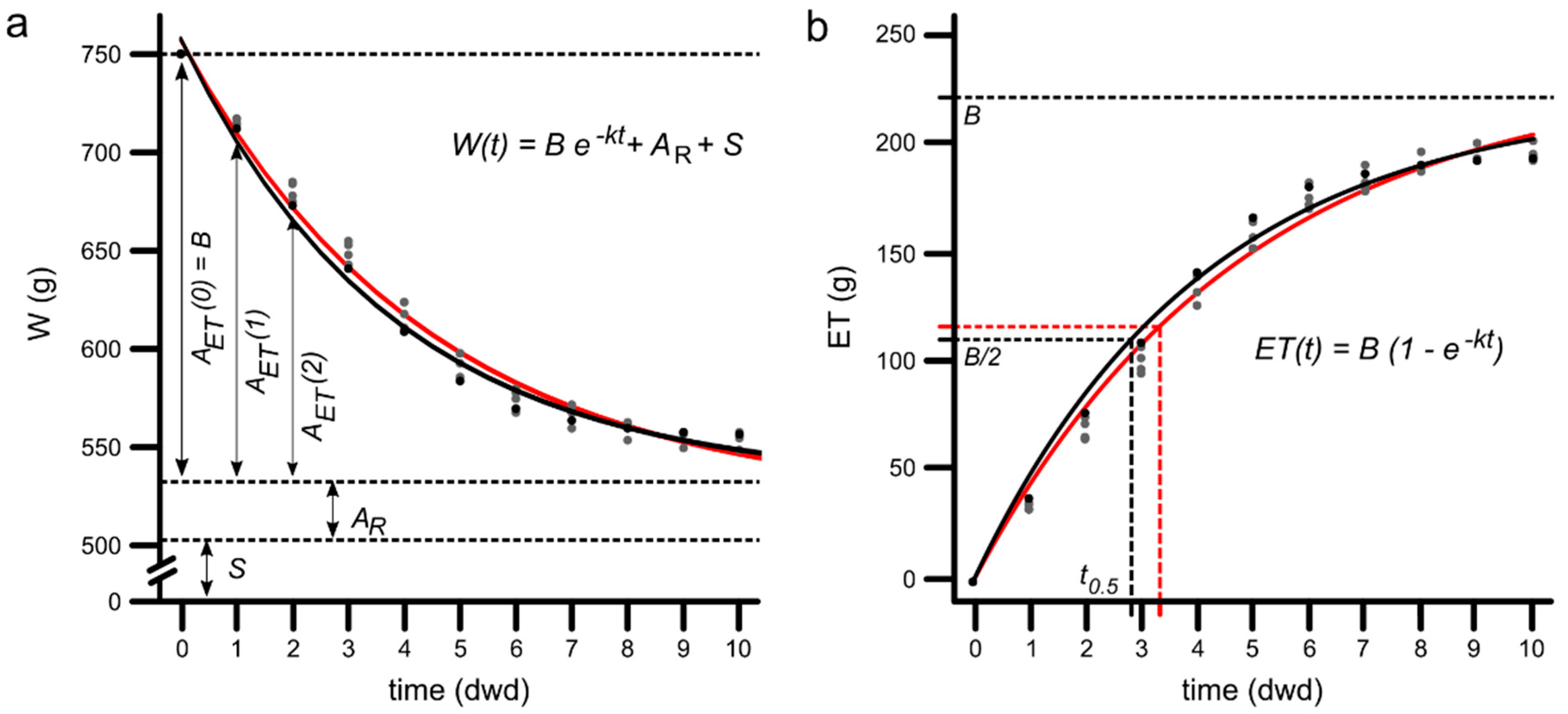
3.1. Mathematical Model Development
3.2. PPS Weight Modelling over Time
3.3. Evapotranspiration Modelling as a Function of Time
3.4. Potential Evapotranspiration Estimated by the Model
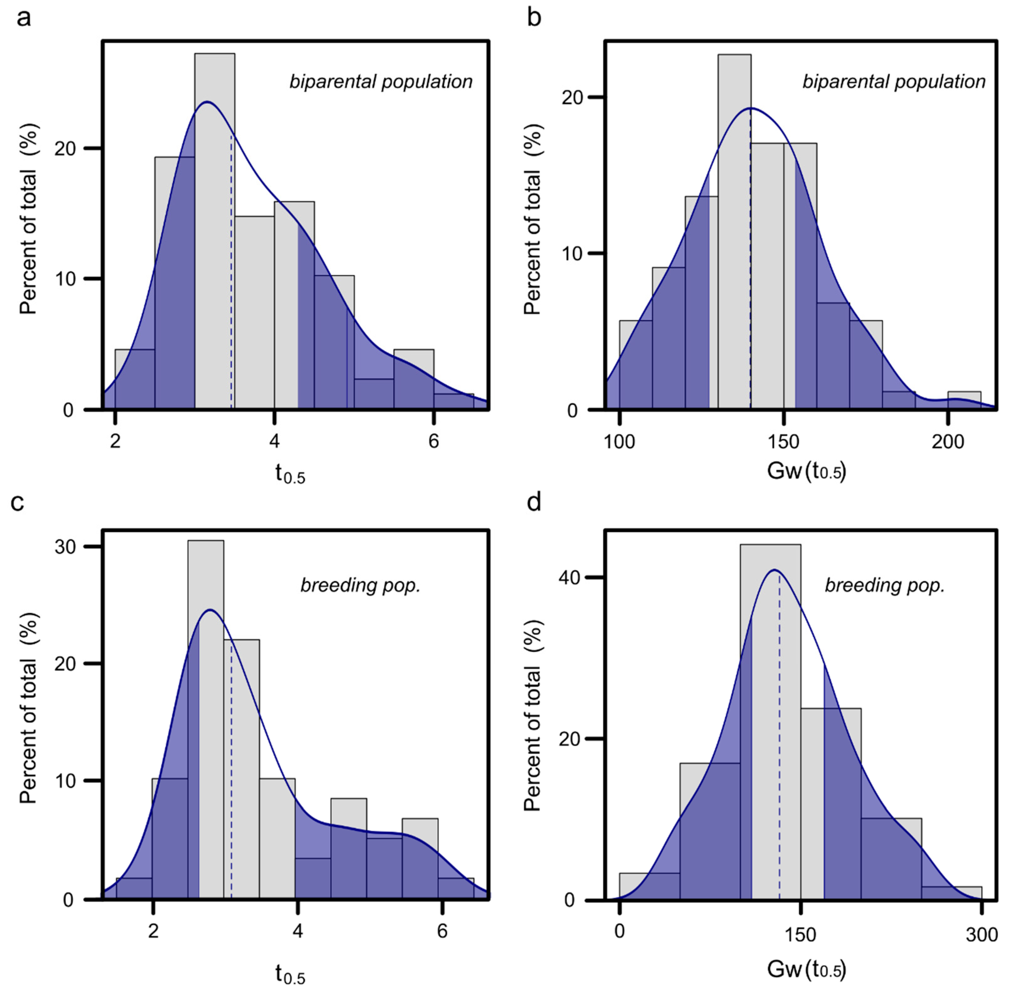
3.5. Half-Time of ET
3.6. Parameters of the ET Model Calculated from the Experiment Data
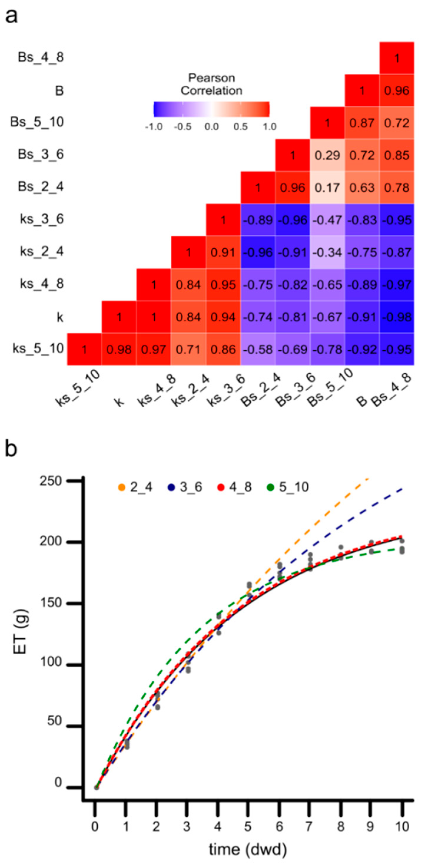
3.7. The Model Minimizes Sampling Requirements in Phenotyping Protocols
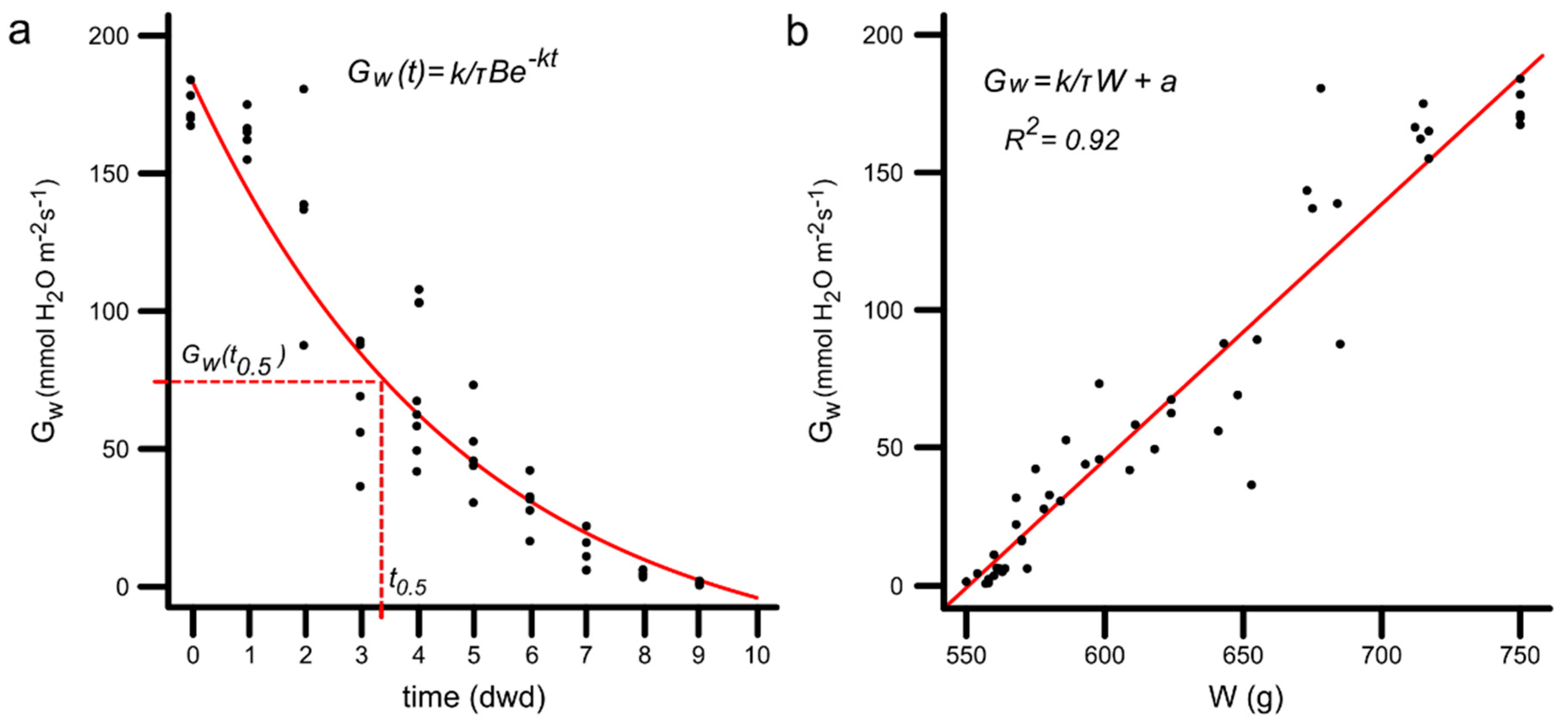
3.8. Stomatal Conductance as a Function of Time
3.9. Conductance as a Function of PPS Weight
3.10. Application of the Phenotyping Methodology in Two Breeding Populations at Different Plant Developmental Stages
3.10.1. Half Time and Stomatal Conductance
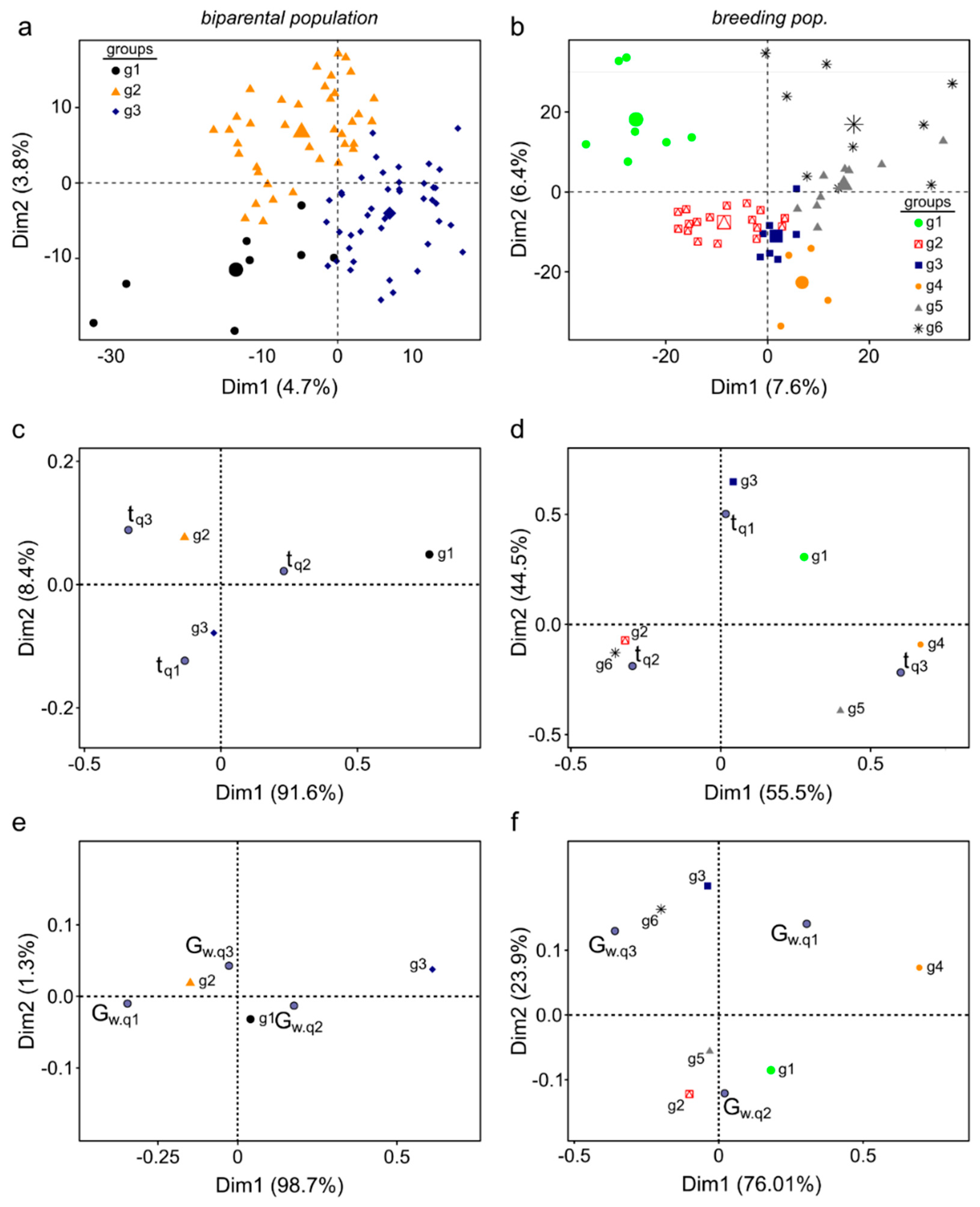
3.10.2. Genetic Structure and Correspondence Analysis
4. Discussion
5. Conclusions
Supplementary Materials
Author Contributions
Funding
Institutional Review Board Statement
Informed Consent Statement
Data Availability Statement
Acknowledgments
Conflicts of Interest
References
- Zhang, T.; Lin, X. Assessing future drought impacts on yields based on historical irrigation reaction to drought for four major crops in Kansas. Sci. Total Environ. 2016, 550, 851–860. [Google Scholar] [CrossRef] [PubMed] [Green Version]
- Zipper, S.C.; Qiu, J.; Kucharik, C.J. Drought effects on US maize and soybean production: Spatiotemporal patterns and historical changes. Environ. Res. Lett. 2016, 11, 094021. [Google Scholar] [CrossRef]
- Boyer, J.S. Crop reaction to water and temperature stresses in humid, temperate climate. In Environmental Stress and Crop Yields; Raper, C., Jr., Kramer, P., Eds.; Westview Press: Boulder, CO, USA, 1983; pp. 3–7. [Google Scholar]
- Kron, A.P.; Souza, G.M.; Ribeiro, R.V. Water deficiency at different developmental stages of glycine max can improve drought tolerance. Bragantia 2008, 67, 43–49. [Google Scholar] [CrossRef] [Green Version]
- He, J.; Du, Y.L.; Wang, T.; Turner, N.C.; Yang, R.P.; Jin, Y.; Xi, Y.; Zhang, C.; Cui, T.; Fang, X.W.; et al. Conserved water use improves the yield performance of soybean (Glycine max (L.) Merr.) under drought. Agric. Water Manag. 2016, 179, 236–245. [Google Scholar] [CrossRef]
- Sinclair, T.R.; Messina, C.D.; Beatty, A.; Samples, M. Assessment across the united states of the benefits of altered soybean drought traits. Agron. J. 2010, 102, 475–482. [Google Scholar] [CrossRef]
- Humplík, J.F.; Lazár, D.; Husičková, A.; Spíchal, L. Automated phenotyping of plant shoots using imaging methods for analysis of plant stress responses-A review. Plant Methods 2015, 11, 29. [Google Scholar] [CrossRef] [Green Version]
- Tuberosa, R. Phenotyping for drought tolerance of crops in the genomics era. Front. Physiol. 2012, 3, 347. [Google Scholar] [CrossRef] [Green Version]
- Vadez, V.; Kholova, J.; Zaman-Allah, M.; Belko, N. Water: The most important “molecular” component of water stress tolerance research. Funct. Plant Biol. 2013, 40, 1310–1322. [Google Scholar] [CrossRef] [Green Version]
- Ratnakumar, P.; Vadez, V.; Nigam, S.N.; Krishnamurthy, L. Assessment of transpiration efficiency in peanut (Arachis hypogaea L.) under drought using a lysimetric system. Plant Biol. 2009, 11, 124–130. [Google Scholar] [CrossRef] [Green Version]
- Zaman-Allah, M.; Jenkinson, D.M.; Vadez, V. A conservative pattern of water use, rather than deep or profuse rooting, is critical for the terminal drought tolerance of chickpea. J. Exp. Bot. 2011, 62, 4239–4252. [Google Scholar] [CrossRef] [Green Version]
- Consoli, S.; Vanella, D. Mapping crop evapotranspiration by integrating vegetation indices into a soil water balance model. Agric. Water Manag. 2014, 143, 71–81. [Google Scholar] [CrossRef]
- Carter, J.N.; Jensen, M.E.; Traveller, D.J. Effect of Mid- to Late- Season Water Stress on Sugarbeet Growth and Yield 1. Agron. J. 1980, 72, 806–815. [Google Scholar] [CrossRef] [Green Version]
- Meyer, W.S.; Green, G.C. Water Use by Wheat and Plant Indicators of Available Soil Water 1. Agron. J. 1980, 72, 253–257. [Google Scholar] [CrossRef]
- Comstock, J.P. Hydraulic and chemical signalling in the control of stomatal conductance and transpiration. J. Exp. Bot. 2002, 53, 195–200. [Google Scholar] [CrossRef] [Green Version]
- Sinclair, T.R.; Holbrook, N.M.; Zwieniecki, M.A. Daily transpiration rates of woody species on drying soil. Tree Physiol. 2005, 25, 1469–1472. [Google Scholar] [CrossRef] [Green Version]
- Belko, N.; Zaman-allah, M.; Cisse, N.; Diop, N.N.; Zombre, G.; Ehlers, J.D.; Vadez, V. Lower soil moisture threshold for transpiration decline under water deficit correlates with lower canopy conductance and higher transpiration efficiency in drought-tolerant cowpea. Funct. Plant Biol. 2012, 39, 306–322. [Google Scholar] [CrossRef] [Green Version]
- Hanks, R.; Shawcroft, R. An economical lysimeter for evapotranspiration studies 1965. Agron. J. 1965, 57, 634–636. [Google Scholar] [CrossRef]
- Pearcy, R.W.; Schulze, E.; Zimmermann, R. Plant Physiological Ecology. Plant Physiol. Ecol. 1989. [Google Scholar] [CrossRef]
- Turner, N.C. Measurement and influence of environmental and plant factors on stomatal conductance in the field. Agric. For. Meteorol. 1991, 54, 137–154. [Google Scholar] [CrossRef]
- Lu, P.; Woo, K.C.; Liu, Z.T. Estimation of whole-plant transpiration of bananas using sap flow measurements. J. Exp. Bot. 2002, 53, 1771–1779. [Google Scholar] [CrossRef]
- Fletcher, A.L.; Sinclair, T.R.; Allen, L.H. Transpiration responses to vapor pressure deficit in well watered “slow-wilting” and commercial soybean. Environ. Exp. Bot. 2007, 61, 145–151. [Google Scholar] [CrossRef]
- Sadok, W.; Sinclair, T.R. Transpiration response of “slow-wilting” and commercial soybean (Glycine max (L.) Merr.) genotypes to three aquaporin inhibitors. J. Exp. Bot. 2010, 61, 821–829. [Google Scholar] [CrossRef] [PubMed] [Green Version]
- Stöckle, C.O.; Kemanian, A.R. Can Crop Models Identify Critical Gaps in Genetics, Environment, and Management Interactions? Front. Plant Sci. 2020, 11, 737. [Google Scholar] [CrossRef] [PubMed]
- Basso, B.; Liu, L.; Ritchie, J.T. A Comprehensive Review of the CERES-Wheat, -Maize and -Rice Models’ Performances; Elsevier Inc.: Amsterdam, The Netherlands, 2016; Volume 136, ISBN 9780128046814. [Google Scholar]
- Gaydon, D.S.; Balwinder-Singh; Wang, E.; Poulton, P.L.; Ahmad, B.; Ahmed, F.; Akhter, S.; Ali, I.; Amarasingha, R.; Chaki, A.K.; et al. Evaluation of the APSIM model in cropping systems of Asia. Field Crops Res. 2017, 204, 52–75. [Google Scholar] [CrossRef]
- Van Den Berg, M.; Driessen, P.M.; Rabbinge, R. Water uptake in crop growth models for land use systems analysis: II. Comparison of three simple approaches. Ecol. Modell. 2002, 148, 233–250. [Google Scholar] [CrossRef]
- Wang, E.; Smith, C.J. Modelling the growth and water uptake function of plant root systems: A review. Aust. J. Agric. Res. 2004, 55, 501–523. [Google Scholar] [CrossRef]
- Camargo, G.G.T.; Kemanian, A.R. Six crop models differ in their simulation of water uptake. Agric. For. Meteorol. 2016, 220, 116–129. [Google Scholar] [CrossRef] [Green Version]
- Rigaud, J.; Puppo, A. Indole-3-acetic catabolism by soybean bacteroids. J. Gen. Microbiol. 1975, 88, 223–228. [Google Scholar] [CrossRef] [Green Version]
- Quero, G.; Simondi, S.; Ceretta, S.; Otero, Á.; Garaycochea, S.; Fernández, S.; Borsani, O.; Bonnecarrère, V. An integrative analysis of yield stability for a GWAS in a small soybean breeding population. Crop Sci. 2021, 61, 1903–1914. [Google Scholar] [CrossRef]
- Song, Q.; Hyten, D.L.; Jia, G.; Quigley, C.V.; Fickus, E.W.; Nelson, R.L.; Cregan, P.B. Development and Evaluation of SoySNP50K, a High-Density Genotyping Array for Soybean. PLoS ONE 2013, 8, e54985. [Google Scholar] [CrossRef] [Green Version]
- R Core Team. R: A Language and Environment for Statistical Computing; R Foundation for Statistical Computing: Vienna, Austria, 2018. [Google Scholar]
- Lê, S.; Josse, J.; Husson, F. FactoMineR: An R Package for Multivariate Analysis. J. Stat. Softw. 2008, 25, 1–18. [Google Scholar] [CrossRef] [Green Version]
- Bates, D.; Mächler, M.; Bolker, B.M.; Walker, S.C. Fitting linear mixed-effects models using lme4. J. Stat. Softw. 2015, 67. [Google Scholar] [CrossRef]
- Russell, L. Emmeans: Estimated Marginal Means, Aka Leastsquares Means; R Package Version 1.4.2; R Foundation for Statistical Computing: Vienna, Austria, 2019. [Google Scholar]
- Kholová, J.; Nepolean, T.; Tom Hash, C.; Supriya, A.; Rajaram, V.; Senthilvel, S.; Kakkera, A.; Yadav, R.; Vadez, V. Water saving traits co-map with a major terminal drought tolerance quantitative trait locus in pearl millet [Pennisetum glaucum (L.) R. Br.]. Mol. Breed. 2012, 30, 1337–1353. [Google Scholar] [CrossRef]
- West-Eberhard, M.J. Phenotypic plasticity and the origins of diversity. Annu. Rev. Ecol. Syst. 1989, 20, 249–278. [Google Scholar] [CrossRef]
- Pigliucci, M. Evolution of phenotypic plasticity: Where are we going now? Trends Ecol. Evol. 2005, 20, 481–486. [Google Scholar] [CrossRef] [Green Version]


Publisher’s Note: MDPI stays neutral with regard to jurisdictional claims in published maps and institutional affiliations. |
© 2022 by the authors. Licensee MDPI, Basel, Switzerland. This article is an open access article distributed under the terms and conditions of the Creative Commons Attribution (CC BY) license (https://creativecommons.org/licenses/by/4.0/).
Share and Cite
Simondi, S.; Casaretto, E.; Quero, G.; Ceretta, S.; Bonnecarrère, V.; Borsani, O. A Simple and Accurate Method Based on a Water-Consumption Model for Phenotyping Soybean Genotypes under Hydric Deficit Conditions. Agronomy 2022, 12, 575. https://0-doi-org.brum.beds.ac.uk/10.3390/agronomy12030575
Simondi S, Casaretto E, Quero G, Ceretta S, Bonnecarrère V, Borsani O. A Simple and Accurate Method Based on a Water-Consumption Model for Phenotyping Soybean Genotypes under Hydric Deficit Conditions. Agronomy. 2022; 12(3):575. https://0-doi-org.brum.beds.ac.uk/10.3390/agronomy12030575
Chicago/Turabian StyleSimondi, Sebastián, Esteban Casaretto, Gastón Quero, Sergio Ceretta, Victoria Bonnecarrère, and Omar Borsani. 2022. "A Simple and Accurate Method Based on a Water-Consumption Model for Phenotyping Soybean Genotypes under Hydric Deficit Conditions" Agronomy 12, no. 3: 575. https://0-doi-org.brum.beds.ac.uk/10.3390/agronomy12030575