Driving Style Assessment System for Agricultural Tractors: Design and Experimental Validation

Abstract

The diffusion of electronics and sensors in agricultural vehicles is enabling a revolution in the field, leading—among the rest—to the introduction of advanced driving-assistance systems (ADAS). From this perspective, the three key performance indicators (KPI) in a tractor are indeed the driving safety, fuel consumption, and operator comfort. Such indexes describe the way the driver interacts with the vehicle, the environment, and other vehicles, respectively. Therefore, such information would be particularly valuable if promptly provided to the driver, e.g., on a dashboard visualizer, so as to adapt the driving style accordingly. Within this context, we propose an algorithmic solution for the on-line estimation of such KPIs. More specifically, by using an off-the-shelf smart-sensor equipped with an Electronic Control Unit (ECU), the chassis accelerations are first processed to extract physics-inspired features and then used to assess the safety and comfort levels; similarly, the speed profile is used to evaluate the economicity of the driving style. The developed method is based upon a cheap setup, and thus it is industrially amenable for its simplicity and robustness. A sensitivity analysis to establish the best sensor placement is finally carried out, together with an extensive experimental campaign considering offroad, urban, and circuit paths.

1. Introduction

The fast pacing diffusion of automatic systems and controls for agricultural tractors is a trend that has been undergoing for decades now: modern tractors are provided with more and more driving assistance features and autonomous systems, as evident from recent works in the area [1,2] but also from a review of future challenges and perspectives in the Internet-of-Things (IoT) [3].

Due to the large masses and relatively high center of gravity, tractors can be very hazardous when traveling on public roads, as highlighted in a research analyzing the Netherlands as a case study [4]; safety issues might indeed occur during agricultural or forestry work, as reported in [5], where an analysis on the agricultural vehicles related to accidents in Portugal is carried out. In particular, the risk of rollover during cornering or when operating on hillsides is among the most relevant safety problems for these machines [5]. As evident from the cited studies, the driving safety is tightly linked to the driver itself and, more specifically, to its driving style.

Left apart from the aforementioned issue, tractors are also particularly critical from the fuel consumption perspective, being characterized by high kinetic energies and provided with many auxiliary subsystems. Again, the effect of the driver on fuel consumption is well known and documented in the literature, being related to aggressive driving behavior, see, e.g., [6,7].

A third key concept when considering agricultural vehicles is indeed the operator comfort: a tractor driver is in fact often required to conduct the vehicle for many hours and in unfavorable conditions [8]. This topic has been and still is of great interest to the scientific community; analyses were conducted about the vibrations measured at the seat according to International Organization for Standardization (ISO) regulations [9,10] but also towards the modeling and consequent prediction of said vibrations, for design purposes [8].

Safety, fuel consumption, and comfort are thus important KPIs to be taken into account when dealing with agricultural vehicles: hence, we propose an algorithmic solution aiming at estimating these quantities in real-time, so as to directly provide the driver with a feedback on how they are driving the vehicle.

Estimating said KPIs means characterizing one’s driving style (DS). The DS assessment for ground vehicles is a relevant problem in the scientific community. Most generally, DS can be defined as the combination of driving skills and behind-the-wheel behavior [11]: this translates into the manner that a driver operates the vehicle (e.g., the steering wheel, throttle, brake pedals, etc.), specific to each person. Driving ability, demographics, surrounding environment, and personality are some human and external factors influencing one’s DS [12,13] and are used to explain the driving behavior. However, considerations regarding such factors are beyond the scope of this research, and while useful for analysis purposes, are not implementable on a real-time assessment system. Similarly, DS distinctions based on road type (e.g., highway or urban) or traffic congestion are not taken into account: detecting such information is not possible with standard tractors’ sensor layouts. A thorough review of the DS recognition techniques has been presented in [14], which well describes the ongoing trends.

This said, DS assessment systems can be principally categorized according to two directions: the employed setup and the chosen methodology. Typical sensor setups include inertial measurement units (IMU) [6,11,15,16], Global Positioning System (GPS) signals [11,17], Controller Area Network (CAN) available signals, e.g., brake or throttle pedal pressure [11,15,18], or even Light Detecting and Ranging (LiDARs) and cameras [16]. Additionally, smartphones have been considered, being an ensemble of the mentioned sensors (typically IMUs and GPS units) [11,19]. Given the particular application, the choice of the sensing setup is indeed critical and not an easy task. A minimal sensor setup will be considered in this article, consisting of an external IMU and only one signal coming from the tractor CAN network, the vehicle speed. Other CAN information, e.g., the steering angle, might be available on some machines. This is however not always guaranteed, as many tractors are still equipped with purely mechanic steering systems, where the angle information is not necessary: hence, in order to guarantee robustness and portability, we limit the set of extracted CAN signals to the sole vehicle speed. Eventually, this minimal setup will prove to be effective for the problem of interest. Indeed, the availability of additional available information could be employed to refine a suitable assessment system: this is however out of scope for this research. GPS units and visual sensors are discarded, as their presence on a production tractor is not guaranteed. With regards to smartphones, their presence is indeed not advisable on tractors, as they might constitute both a distraction from the agricultural activity and a safety hazard.

On the other hand, different methodologies have been used, with a first set of approaches employing machine-learning methods [15,16,19,20] and a second one resorting to physics inspired, rule-based, or model-based algorithms [6,11,21]. The authors in [19] developed an assessment system involving maneuver, car type, and traffic conditions classification, building a cascade-like algorithm scheme relying on different algorithms, e.g., perceptrons, k-nearest neighbors, and decision trees. In [15], an unsupervised learning approach is proposed, based upon signals extracted from the CAN bus, and considering more than 50 drivers: however, the presented approach is thought to be performed off-line, since data are recorded on a data-logger and then processed later on. In other recent contributions [16], the authors use Hidden Semi-Markov Models to extract driving patterns from data, and an interesting comparison among different drivers is also detailed. Nonetheless, the proposed method is based on signals coming from a camera, which is usually not present on today’s industry-grade tractors; additionally, the algorithm is not specifically designed to be implemented in a real-time environment. Furthermore, although being usually extremely well performing, model-free approaches heavily relying on machine learning algorithms are well known to lack in robustness, especially when tested over events not present in the training set: this is a critical issue when coming to agricultural tractors from an implementation-oriented perspective. In fact, vehicle payload might change significantly [22], as different tools or trailers might be connected to the vehicle front or rear part, thus potentially yielding unpredictable results.

Physics-based and rule-based approaches are instead more suitable for the considered application. In [6], the author employs a simplified longitudinal model of the vehicle to estimate the energy (or fuel) consumption for a given speed profile: this information is then used to construct an economy index. Even though the described approach is effective, some introduced assumptions are not valid in case of tractors. The authors in [21] conduct a preliminary analysis for the safety assessment in ground vehicles, based on a smartphone setup; given a pre-trained safe region in the $x-y$ accelerations plane, the data points within or outside this region are evaluated. The investigation is indeed interesting, and an experimental validation for different drivers is provided: however, the authors do not distinguish between unsafe points, attributing the same importance to data outside the safe region, regardless of the acceleration magnitude. A more recent study [11], presents a combined assessment of safety, economy, and comfort, which is of interest to us for the previously mentioned reasons; a set of Controller Area Network (CAN) retrieved signals—including, e.g., steering wheel angle and brake pressure—and a GPS unit are employed. The authors computed eight empirical indicators: some of them include, e.g., the average driving speed over the limit during the ride, assuming the knowledge of information about the road type (so as to establish the speed limit), which is not available on every tractor. Eventually, the author proposed a computation of the indices based on a nonlinear function of the features. The proposed formulae are however purely empirical, and no further explanations are provided on, e.g., the decision of including the vertical jerk in the assessment of fuel consumption. Moreover, the definition of “expert” reference values for the computed features is never explained in details. For these reasons, the study in [11], while indeed being interesting, lacks clarity in different points and fails at delivering a sound physics-inspired estimation of the three indices.

Having established the driving factors for this research, and having documented the existing state-of-the-art, the most significant contributions covered by this manuscript follow:

• We design a complete driving scoring system for an agricultural tractor, including the computation of an Eco Index (fuel consumption), a Safety Index, and a Comfort Index. To the best of our knowledge, this is the first time that an assessment system for the concurrent evaluation of these three KPIs starting from physics-inspired considerations is carried out.
• The DS assessment problem is applied for the first time to tractors; this case study requires a series of special considerations, which are carefully addressed throughout the manuscript.
• A real-time oriented solution is developed, based on a very simple sensor setup, possibly encompassing a wide variety of tractors. We thus enhance both the industrial relevance and the reproducibility of the scientific output. Moreover, a sensitivity analysis with respect to the best sensor placement is carried out.
• An experimental calibration is proposed so as to map the indices into a human-understandable scoring, i.e., 0–100 KPIs: this point is mandatory when designing an operator-oriented solution, having to display the transduced sensor information directly to the driver.

Indeed, the proposed KPIs are not exact or unique, in the sense that the quantities under analysis cannot be quantitatively assessed. Starting from the state-of-the-art, we propose some modifications to the existing research basis, resorting to common sense reasoning and inspired by the actual availability of sensors.

The remainder of the article is as follows. The experimental setup is described in Section 2, and in Section 2.1 the driving style assessment problem is defined and declined in its three components. The algorithm validation campaign is then described and discussed in Section 3; Section 4 draws some final considerations.

2. Materials and Methods

The vehicle employed in the research is represented in Figure 1: it is provided with three six degrees-of-freedom (DOF) inertial measurement units (IMU), one on the cabin deck (Figure 1d), another one on the steering column (dashboard, Figure 1c), and the last one on the seat. The IMUs are identical: the first two sensors are employed so as to understand the better placement for the problem of interest, since only one sensor is to be used for the final implementation. On the other hand, the seat IMU will serve as a validation tool for the comfort assessment (Section 3.1). The sensors measure the three accelerations and the three angular velocities along their orthogonal axes ($a_x$, $a_y$, $a_z$, ${\omega }_x$, ${\omega }_y$, ${\omega }_z$) at a sampling frequency $f_s$ = 100 Hz; a pre-processing phase on such measurements is necessary in order to obtain meaningful acceleration signals. Namely, the sensor frames need to be rotated and aligned to the tractor frame.

The IMUs are provided with an integrated electronic control unit (ECU) and a CAN board: in this way the algorithm is directly embedded inside the sensor—running at frequency $f_s$—and the only required external signal is the vehicle speed (v), based on wheel encoder measurements, retrieved from the CAN network and made available to the algorithm.

Finally, the tests are performed connecting a trailer to the tractor, as shown in Figure 1b, so as to consider a more realistic validation phase.

2.1. Driving-Style Assessment Algorithm

As mentioned in Section 1, the driving style for an agricultural tractor can be characterized by safety, comfort, and economy components. The developed estimation scheme is represented in Figure 2: the first step consists in pre-processing the measured accelerations, while the three indices are then computed according to a different set of signals. A supervisor is in charge of keeping track of the beginning and the end of a driving section.

2.1.1. Pre-Processing

In order to obtain an informative set of acceleration measurements, we have to rotate the sensor frames aligning them to the tractor frame, with the x-axis pointing towards the front of the tractor; the z-axis pointing upwards, exiting from the cabin; and the y-axis completing the orthogonal frame. The sensors are mounted such that the yaw angle offset is ≈0${}^{\circ }$ with respect to the tractor frame; hence, an estimation and successive compensation for the roll and pitch mounting angles is carried out according to the procedure detailed in [23].

2.1.2. Eco Index

The economicity of an operator driving style is related to the fuel consumption; it is well known that higher fuel consumption is in fact related to aggressive driving behavior [7], especially in terms of sudden accelerations and braking events, i.e., associated with fast speed fluctuations.

Inspired from [6], an economic driving style is characterized by a band-limited speed profile, which can be obtained by low-pass filtering the original signal. Then, given a speed profile, the vehicle energy dissipation along a certain driving path can be computed through a simplified longitudinal dynamics model

$$M_{veh}\dot{v}\left(t\right)=-{\gamma }_{fri}v\left(t\right)+F_{eng}\left(t\right)-F_{brake}\left(t\right)-M_{veh}gsin\left(\varphi \left(t\right)\right)$$

(1)

whereas ${\gamma }_{fri}·v$ is a lumped friction term, an acceptable modeling assumption for our purposes [22]; g is the gravity acceleration; $\varphi$ is the road inclination angle; $M_{veh}$ is the tractor payload; and $\dot{v}$ is the time derivative of v, which can be computed through a derivative filter. The time dependence $\left(t\right)$, explicit in (1), will be dropped from now on for the sake of simplicity. The gravity contribution is neglected in [6], assuming flat road conditions: however, such an assumption is not acceptable in the case of agricultural vehicles, which are often operated on slopes. Hence, the road inclination angle is estimated through a Kalman Filtering approach [23], resorting to the available acceleration measurements ($a_{x,y,z}$), angular rates (${\omega }_{x,y,z}$), and vehicle speed (v).

The friction term will be on the other hand neglected [6]; given the large mass and relatively low travel speed—limited at 40 km/h—of the vehicle, the dominant terms are the inertial and gravity ones. Thus, the longitudinal balance of powers is obtained by multiplying both sides of (1) by v:

$$P_{eng}-P_{brake}=F_{eng}v-F_{brake}v=M_{veh}v\left(\dot{v}+gsin\left(\varphi \right)\right).$$

(2)

When the left-hand side term in (2) is positive, the engine is providing power so as to propel the vehicle and is thus consuming fuel in the process. Hence, by integrating the quantity on the right-hand side of (2) only when positive values occur, an estimate for the tractor specific energy consumption can be obtained as:

$$\begin{array}{cc}\hfill e_{loss}& ={\displaystyle \frac{E_{loss}}{M_{veh}}}={\int }_{t_s}^{t_e}{\tilde{P}}_{loss}dt\hfill \\ \hfill {\tilde{P}}_{loss}& =\begin{array}{c}\left\{\begin{array}{cc}v\left(\dot{v}+gsin\left(\varphi \right)\right)\hfill & ,\dot{v}+gsin\left(\varphi \right)>0,\hfill \\ 0\hfill & ,\dot{v}+gsin\left(\varphi \right)\le 0.\hfill \end{array}\right.\end{array}\hfill \end{array}$$

(3)

The estimation of the specific (mass normalized) energy consumption is another difference with respect to [6]: in this way, robustness with respect to mass is enforced, as the same might change significantly, e.g., in the presence of ballasts or trailers.

At this point, we need to assess the difference between the actual energy consumption and the one occurring in ideal conditions; in order to do so, a first-order low-pass filter is introduced so as to estimate the ideal speed profile, whose pole $f_{lp}^{EI}$ is a tuning knob. The ideal speed and speed rate profiles calculated through the low-pass filter are to be plugged into (3) in order to compute the ideal energy loss $e_{loss}^{id}$, opposed to the real one, $e_{loss}^{re}$. An example of the computed speed and speed rate ideal and real profiles is provided in Figure 3a,b, for Eco and not-Eco tests, respectively. One can note that the ideal and real profiles are practically identical in the first test, meaning that the driver is leading the machine in an economical way. Significant differences are noticeable in the second one, and the low-pass filter is effectively attenuating the high frequencies associated with not-economic driving.

At this point, the Eco Index is computed according to the following relation:

$$E{I}_{raw}=e_{loss}^{re}-e_{loss}^{id}.$$

(4)

Note that the higher the value of $E{I}_{raw}$, the less economic is the driving; this convention is maintained also for the other indices. It is clear that the integrals in (4) need to be carefully treated for a twofold reason:

• Integrals drift is a common problem when integrating real-world raw data (the speed signal is not high-pass filtered; thus, a constant measurement error might translate in huge errors due to the integration process in (3)) [24]. Integrating over a driving session $t_e-t_s$—which might last several hours for an agricultural tractor—is hence to be avoided.
• In order to obtain an easily comparable scoring, i.e., among different driving sessions, it is necessary to reset the index computation upon reaching certain conditions. In this research a reset based on the traveled distance (d) is introduced. By resetting the integrals we also ensure that particularly dangerous maneuvers are not hidden by a subsequent series of safe ones.

As soon as $d={\int }_0^{t}vdt\ge \overline{d}$, reset is enforced. $\overline{d}$ is a design parameter, fixed to 1000 m.

Finally, in order to obtain a readily understandable scoring, i.e., in a 0–100 scale, let us introduce a scaling function $f_{EI}$ such that:

$$EI=f_{EI}\left(E{I}_{raw}\right),$$

(5)

where the scaling factor needs to be identified from a set of experiments, which are described in detail in Section 2.2.

A schematic representation of the described computation algorithm is provided in Figure 4.

2.1.3. Safety Index

Driving safety is tightly related to planar accelerations of the vehicle; indeed, these measurements influence the friction ellipse, defining the adherence characteristic of the machine, and depending in turn on the tire and terrain features (e.g., dry asphalt, snow, …) [21]. Typical unsafe maneuvers both excite longitudinal and lateral vehicle dynamics, with an example being a strong braking action while cornering.

Hence, the design of a Safety Index estimator should take into account these accelerations: the approach proposed herein is inspired from the concept of the safe-driving region in the $x-y$ accelerations plane, originally proposed in [21] for road vehicles applications. However, the present work constitutes an innovation with respect to the mentioned reference for different reasons:

• We include a loss function, penalizing both the occurring of acceleration points outside the safe region and the distance of said points from the region.
• A different experimental layout (see Section 2) is employed in this work, and a processing phase is introduced so as to cope with intrinsic measurement noise associated to inertial measurements and to low-frequency acceleration biases due to road grade. In [21], no filtering phase is considered, since road vehicles are less likely to be operated on inclines while being also less subject to high frequency vibrations influencing the acceleration spectra.
• The Safety Index is here real-time computed and converted into a human understandable score.

Remark 1.

The planar accelerations are informative measurements of the vehicle dynamics. Indeed, if one considers, e.g., an increased payload for the machine, the underlying system model would change—this is easily verified from Equation (1). Consequently, the same driver inputs would result in different responses in terms of acceleration. As one could intuitively understand, this means that one should properly modulate the vehicle commands so as to produce moderated accelerations and avoid dangerous events. The driver inputs are indeed very important when classifying the driver behavior [25], which is however not the scope of this research.

IMU measurements are composed of different contributions: high frequency ones, due, e.g., to engine vibrations or ground asperities, and low-frequency ones, due, e.g., to ground slope and banking. Among such contributions, we need to extract the one related to the driver actions, in order to characterize driving safety: a solution consists in accurately filtering the signals.

Figure 5a shows the measured longitudinal and lateral accelerations in an unsafe drive experiment; the driver contribution is distinguishable among the high-frequency noise, which is particularly unfavorable for the dashboard sensor. On the other hand, measured accelerations are also characterized by quasi-constant terms due to the ground slope, which has to be taken care of, in order to achieve a consistent representation of the driver-effect in the frequency spectrum. For these reasons, a band-pass filtering is here introduced to treat the raw acceleration signals: a low frequency pole is in charge of filtering off the ground offsets, while two higher frequency poles take care of the high-frequency content highlighted in Figure 5a.

$$F_{SI}\left(s\right)={\displaystyle \frac{{\left(2\pi f_{lp}^{SI}\right)}^2}{{\left(s+2\pi f_{lp}^{SI}\right)}^2}}·{\displaystyle \frac{s}{s+2\pi f_{hp}^{SI}}}.$$

(6)

As one can note from Figure 5b, the $SI$-filtered signals are very similar for the two sensors, meaning that the same information can be extracted starting from two different placements, given that a suitable processing is performed onto the signals.

At this point, the filtered acceleration vector ${\overrightarrow{a}}^{SI}=\left[a_x^{SI},a_y^{SI}\right]$ is processed in order to extract safety-oriented signals features.

The vector is compared to a g-g plot like safe driving region $\mathrm{{\rm Y}}$, Figure 6. Two experiments, a safe and an unsafe driving one, are superimposed on the figure: the differences among the tests are evident, and the percentage of data points within $\mathrm{{\rm Y}}$ is reported in the legend for both experiments. $\mathrm{{\rm Y}}$ is defined as:

$$\mathrm{{\rm Y}}=\left\{\left(a_x,a_y\right)\in {\mathbb{R}}^{2}s.t.{\underline{a}}_x\le a_x\le {\stackrel{̲}{a}}_x\wedge {\underline{a}}_y\le a_y\le {\stackrel{̲}{a}}_y\wedge a_x\le {\displaystyle \frac{k}{a_y}}\wedge a_x\le {\displaystyle \frac{k}{-a_y}}\right\}$$

(7)

where the ∧ sign represents a logic AND between two expressions. The tunable box bounds ${\stackrel{̲}{a}}_x,{\underline{a}}_x,{\stackrel{̲}{a}}_y,{\underline{a}}_y$ enforce a limit on the maximum (traction) and minimum (braking) longitudinal accelerations and on the maximum and minimum lateral accelerations during cornering. Moreover, the hyperbole branches parameterized by k are introduced so as to pose a limit stricter than the box bounds on mixed conditions, i.e., excitation of both longitudinal and lateral dynamics.

Remark 2.

Note that the parameters defining Υ are specific to the tractor physical and geometrical parameters but most importantly to the safety perception of the vehicle tester, given that an objective assessment of this quantity does not exist. The tester is in fact in charge of giving a feedback on the perceived accelerations, establishing reference acceleration values to be considered as “safe”. More details regarding the calibration of Υ are given in Section 2.2.

The acceleration components $\left(a_x^{SI},a_y^{SI}\right)$ are then penalized according to their distance from $\mathrm{{\rm Y}}$; indeed, if the point is contained in $\mathrm{{\rm Y}}$, we do not penalize it. Hence, let us consider the limit acceleration vector (see Figure 6):

$${\overrightarrow{a}}^{lim}=\left[a_x^{lim}{a}_y^{lim}\right],$$

(8)

which is defined according to the following rules:

$${\displaystyle \frac{a_y^{lim}}{a_x^{lim}}}={\displaystyle \frac{a_y^{SI}}{a_x^{SI}}}=m,sign\left(a_x^{lim}\right)=sign\left(a_x^{SI}\right),sign\left(a_y^{lim}\right)=sign\left(a_{lim}^{SI}\right),\left(a_x^{lim},a_y^{lim}\right)\in \mathrm{{\rm Y}}.$$

(9)

Equations in (9) enforce the same direction and orientation for the two vectors. The features $a_{id}$ and $a_{re}$ are obtained according to:

$$a_{id}=min\left({\left|\left|{\overrightarrow{a}}^{lim}\right|\right|}_2,{\left|\left|{\overrightarrow{a}}^{SI}\right|\right|}_2\right),a_{re}={\left|\left|{\overrightarrow{a}}^{SI}\right|\right|}_2.$$

(10)

The two quantities in (10) are of intuitive physical interpretation: the first one represents the limitation of the instantaneous acceleration vector to the safe region, and the second one is its module. Now, let us consider the penalty function $\Delta a=a_{re}-a_{id}$; in this way, the acceleration points outside $\mathrm{{\rm Y}}$ are penalized according to the distance from the same. The Safety Index is computed as a function of $\Delta a$:

$$S{I}_{raw}\left(a_{id},\Delta a\right)={\displaystyle \frac{{\int }_{t_s}^{t_e}{e}^{\Delta a}-1dt}{{\int }_{t_s}^{t_e}{e}^{\Delta a}-1+a_{id}dt}}\in \left[0\right.,\left.1\right).$$

(11)

Note that for $\Delta a=0$, i.e., for a perfectly safe driving profile, $S{I}_{raw}=0$, thanks to the introduction of the constant term 1. Moreover, the introduction of an exponential penalty is necessary so to strongly penalize the points very far from the safe boundaries, even within an overall safe driving profile.

An interesting property of $S{I}_{raw}$ is the boundedness of the same between 0 and 1, whereas 0 corresponds to a completely unsafe driving style, i.e., ${\overrightarrow{a}}^{SI}\in \mathrm{{\rm Y}}\forall t$, and 1 corresponds to a perfectly safe one.

Additionally, in this case, let us introduce the reset specified for the Eco Index in Section 2.1.2, so as to obtain a comparable scoring.

The overall safety index assessment module is depicted in Figure 7. Finally, we introduce a scaling function $f_{SI}$, as shown for the Eco index in Equation (5).

2.1.4. Comfort Index

The comfort problem is of paramount importance in agricultural vehicles, where operators are often required to drive for many hours and in unfavorable conditions [8]. Agricultural vehicles driving comfort is regulated according to the ISO 2631-1:1997 standard [26], which establishes the most significant range of frequencies (0.5–80 Hz) directly transmitted to the whole body in a seated position. For frequencies below 0.5 Hz, the body reacts as a rigid element, while those higher than 80 Hz are damped by the outer layers of the body. In the defined range of frequencies, relative displacements among the organs occur, which are potentially dangerous for the driver’s health. Given that the refresh frequency of the sensors is 100 Hz, we limit the band of the signals at 50 Hz, rather than 80 Hz, so as to prevent the aliasing phenomenon. The band limiting is enforced through a first-order Butterworth filter. Within the considered frequency band, ISO standards define a set of weighting transfer functions, in order to emphasize the most relevant sections of the acceleration spectra determining of human comfort.

Two different filters, one for the x and the y axis and one for the z axis are thus defined as follows:

$$\begin{array}{cc}\hfill F_{CI}^{xy}\left(s\right)& ={\displaystyle \frac{s/{\Omega }_{xy}+1}{s^2/{\Omega }_{xy}^2+s/\left({\Omega }_{xy}{q}_{xy}\right)+1}},\hfill \\ \hfill F_{CI}^z\left(s\right)& ={\displaystyle \frac{s/{\Omega }_{z,1}+1}{s^2/{\Omega }_{z,1}^2+s/\left({\Omega }_{z,1}{q}_{z,1}\right)+1}}·{\displaystyle \frac{s^2/{\Omega }_{z,2}^2+s/\left({\Omega }_{z,2}{q}_{z,2}\right)+1}{s^2/{\Omega }_{z,3}^2+s/\left({\Omega }_{z,3}{q}_{z,3}\right)+1}},\hfill \end{array}$$

(12)

where $q_{xy},{\Omega }_{xy}$, $q_{z,1,2,3}$, and ${\Omega }_{z,1,2,3}$ are provided in [26].

The root mean square value of the frequency-weighted and band-limited accelerations $a_{x,y,z}^w$ is then computed as:

$$rm{s}_{x,y,z}=\sqrt{{\displaystyle \frac{1}{t_s-t_e}}{\int }_{t_s}^{t_e}{\left(a_{x,y,z}^w\right)}^{2}dt}$$

(13)

The obtained values are used to compute the Estimated Vibration Dose Value ($eVDV$), considering the maximum of the three $rms$ values and weighting it by the driving session time. The Comfort Index is then equal to $eVDV$:

$$C{I}_{raw}=eVDV={\left(t_e-t_s\right)}^{0.25}·max(rm{s}_x,rm{s}_y,rm{s}_z),$$

(14)

Due to the presence of the driving time term, the longer the session, the less comfortable the driving is assessed to be. Additionally, the $max\left(\right)$ function extracts the worst-case acceleration contribution, so as to consider vibration components in each one of the three axes. Note that (14) is slightly different from the formulation described in [26], which contains other scaling constants: given that we are interested in assessing the comfort on a 0–100 scale, such scaling constants are discarded.

The same considerations carried on for the Eco and Safety indices apply here: a scaling $f_{CI}\left(C{I}_{raw}\right)$ is introduced so as to obtain an human understandable score, and the calibration procedure for the said function is reported in Section 2.2.3.

A schematic representation of the Comfort Index computation algorithm is provided in Figure 8.

Finally, let us remark that the comfort metrics should be computed by exploiting the accelerations felt by the driver. Placing an IMU onto the seat is however impractical for an industry-oriented implementation; therefore, a proxy of the driver-referenced accelerations is to be found in the available measurements (i.e., the deck and dashboard IMUs). In practice, the only difference between the accelerations at the cabin deck level and those at the seat is the presence of a suspension system, typically modeled as a spring-damper [27]. We will show in Section 3 that the proxy is acceptable for our purposes, while Section 2.2.3 will highlight as the dashboard IMU is not suitable for the comfort assessment.

2.1.5. Supervisor

A supervisor block is designed so as to manage the reset logic described in Section 2.1.2 and the indices scaling through functions $f_{SI}$, $f_{EI}$, and $f_{CI}$. Moreover, the supervisor stops the integration of the indices and resets their values whenever the vehicle stops for more than 10 s, assuming that the driving session has been stopped or paused.

2.2. Algorithm Calibration

The algorithms proposed in Section 2.1 are based upon different parameters, which need to be tuned; we thus discuss the calibration procedure for the different algorithm modules. Most importantly, the value of the computed raw indices is not meaningful per-se, and it is necessary to tune the rescaling functions $f_{EI,SI,CI}$.

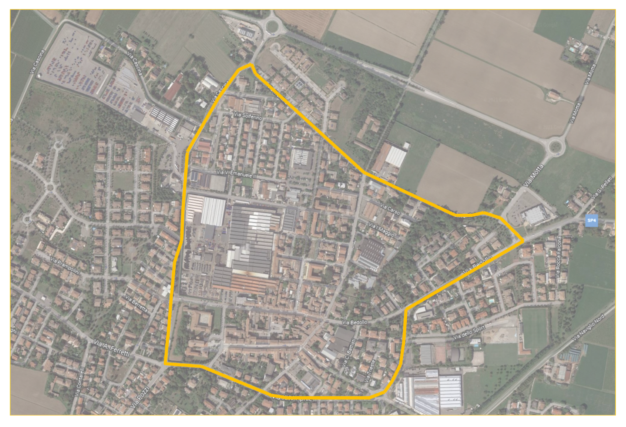
The calibration tests have been performed on a circuit (see Figure 9 for a satellite image of said circuit), so as to improve repeatability. A professional tractor driver was employed in the experiments; the driver has been instructed on how to perform the tests, in order to excite the characteristics of interest.

For the Comfort Index calibration, two additional tests have been considered, over offroad tracks. An example for the first of the two offroad paths is provided in Figure 10. The other considered path is similar to the one represented in Figure 10, while being significantly bumpier.

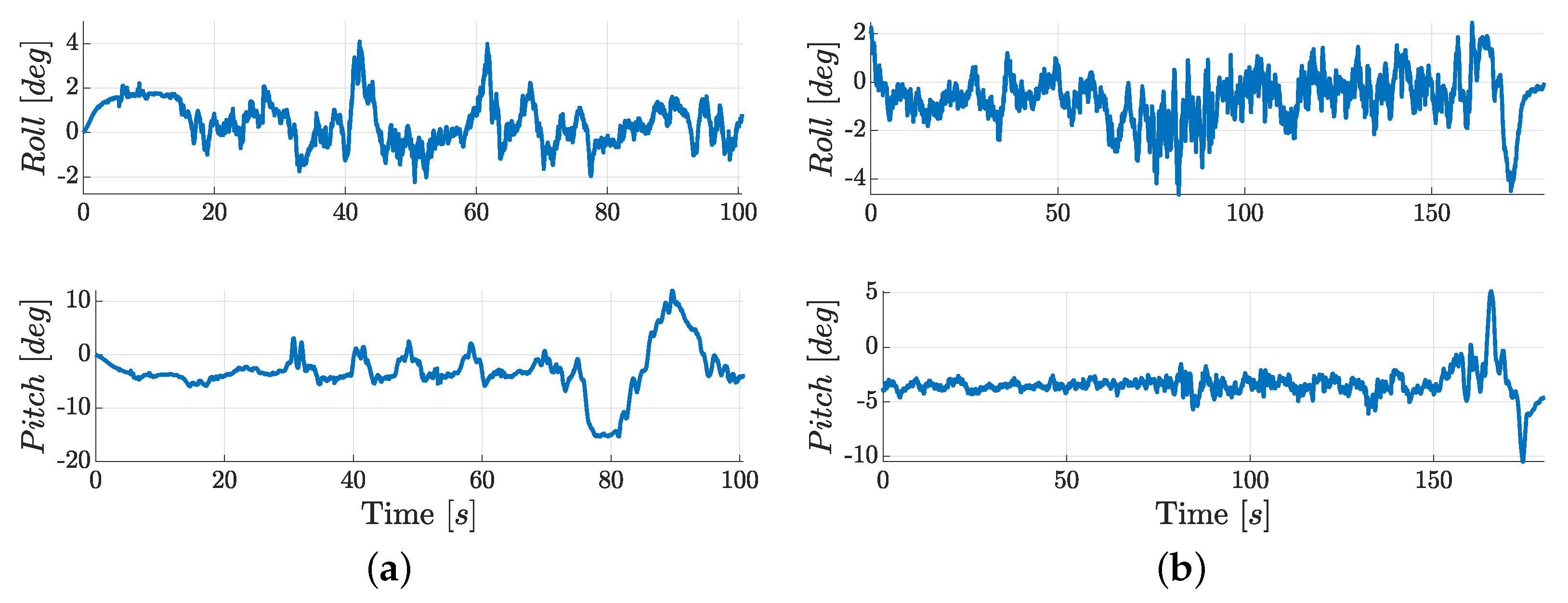
Finally, the circuit tests are indeed characterized by a flat road, with an overbridge, yielding significant vehicle pitching (up to −15${}^{\circ }$); see Figure 11a; the bridge is at ≈80 s. Offroad tests are instead characterized by relatively plain surfaces, with small slopes/banking. An example is provided in Figure 11a, showing the attitude angle values for the experiment on the gravel path in Figure 10.

Remark 3.

Note that it is not possible to define an absolute and “objective” assessment of Safe and Eco drive, whereas a quantitative evaluation of the Comfort comes from the ISO regulations. For this reason, we rely on the driver expertise for the calibration of the Safety and Eco modules, while the $eVDV$ raw value (see (14)) is considered to be an informative representation of the less-comfortable and more-comfortable tests.

2.2.1. Eco Index

In order to calibrate the Eco Index, three tests are performed: in the first experiment, $T_{eco,1}$, the tester is asked to maintain an Eco drive style, while in the two other sessions ($T_{eco,2}$ and $T_{eco,3}$) the non-eco features are gradually highlighted, with strong accelerations and frequent restarts. The low-pass filter pole $f_{lp}^{EI}$ is a key tuning parameter; intuitively, the lower is the pole, the less tolerant the algorithm will be in determining the ideal eco driving style. The value for $f_{lp}^{EI}$ is chosen such that, in test $T_{eco,1}$ (see Figure 3a)—which should be the reference for an ideal speed profile—the root mean square percentage error between v and $v_{id}$ should be smaller than the 10%:

$$rm{s}_{\%}=100·{\displaystyle \frac{\sqrt{{\sum }_{i=1}^{N_s}{\left(v\left(i\right)-v_{id}\left(i\right)\right)}^2}}{\sqrt{{\sum }_{i=1}^{N_s}{\left(v\left(i\right)\right)}^2}}}\le 10.$$

(15)

$f_{lp}=0.01\mathrm{Hz}$ guarantees that (15) is verified.

With regards to the function $f_{EI}$, an a-priori score is assigned to the three experiments: the most Eco test (based on the driver expertise) is assigned with the score $E{I}_{low}=15\%$; the next one is evaluated $E{I}_{mid}=50\%$; while the last one $E{I}_{high}=85\%$. At this, point $E{I}_{raw}$ is computed for three tests, by taking the value obtained for the three driving sessions $E{I}_{raw,1,2,3}$. A Least Squares problem is then solved, and the best-fitting function is found to be a first-order polynomial (Figure 12)

$$\left[\begin{array}{c}E{I}_{raw,1}\\ E{I}_{raw,2}\\ E{I}_{raw,3}\end{array}\right]·k_{EI}=\left[\begin{array}{c}E{I}_{low}\\ E{I}_{mid}\\ E{I}_{high}\end{array}\right].$$

(16)

Overall, a fitting error of ≈5% is obtained, thus minimizing the distortion between the raw score and the scaled one. Let us note that $E{I}_{low}$ and $E{I}_{high}$ have been set with some tolerance with respect to $0\%$ and $100\%$: this is necessary so as to allow worse or better scoring with respect to the calibration ones. Finally, a saturation on the scaling function is introduced, and the complete formula reads:

$$\begin{array}{cc}\hfill f_{EI}\left(E{I}_{raw}\right)& =\begin{array}{c}\left\{\begin{array}{cc}{k}_{EI}·E{I}_{raw}\hfill & ,E{I}_{raw}\le 100/k_{EI},\hfill \\ 100\hfill & ,E{I}_{raw}>100/k_{EI}.\hfill \end{array}\right.\end{array}\hfill \end{array}$$

(17)

2.2.2. Safety Index

Similarly, as previously discussed for the Eco Index, the driver is instructed to perform three experiments, $T_{safe,1}$, $T_{safe,2}$, and $T_{safe,3}$, in which the unsafe features—e.g., accelerating or braking while cornering—are gradually increased, starting from the first test, which is the safest one: hence, also in this case the assessment of a qualitative Safe driving is left to the driver expertise.

First, the $\mathrm{{\rm Y}}$ region parameters ${\underline{a}}_{x,y}$, ${\stackrel{̲}{a}}_{x,y}$, and k in (7) need to be calibrated; this calibration is to be carried on for both the considered sensors, namely, the dashboard IMU and the deck one.

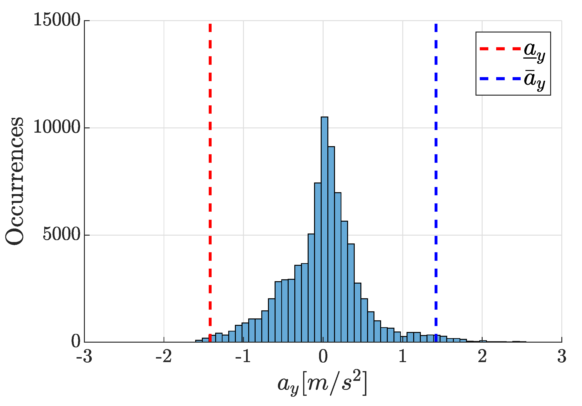
Let us consider the first test among the three, which is the safest one—according to the driver experience. The chosen tuning rule is such that, for the longitudinal acceleration, ${\underline{a}}_x$ and ${\stackrel{̲}{a}}_x$, respectively, represent the 1st and the 99th quantiles for the distribution of $a_x^{SI}$ in such a test. For the lateral acceleration, ${\underline{a}}_y=-{\stackrel{̲}{a}}_y$—since no difference should exist between left and right turning—and they are computed as the mean between the absolute values of the 1st and 99th quantiles in said safe driving test: the distribution of the lateral acceleration data measured at the deck, in the safe drive test, is provided in Figure 13. With regards to k, its value is selected such that, in test $T_{safe,1}$, $95\%$ of the data points $\left[a_x^{SI},a_y^{SI}\right]$ belong to $\mathrm{{\rm Y}}$: $k=1$ satisfies this condition for both sensors.

Finally, in order to select the proper scaling function $f_{SI}$ so as to transform the raw indices in a 0–100% value, the same procedure carried on for the Eco Index in Section 2.2.1 is employed here. Eventually, we get two different functions for the two sensors (Figure 14), and the structure of the selected function, which is a first order polynomial, reads:

$$\begin{array}{cc}\hfill f_{SI}\left(S{I}_{raw}\right)& =\begin{array}{c}\left\{\begin{array}{cc}{k}_{SI}·S{I}_{raw}\hfill & ,S{I}_{raw}\le 100/k_{SI},\hfill \\ 100\hfill & ,S{I}_{raw}>100/k_{SI}.\hfill \end{array}\right.\end{array}.\hfill \end{array}$$

(18)

As one can note from Figure 14, there are no significant differences when considering dashboard or deck IMUs in the safety assessment: this is however due to the accurate signal-processing phase. Both positions could be in principle used for the assessment of safe driving.

2.2.3. Comfort Index

With regards to the comfort index, a slightly different approach is considered, recalling Remark 3. Taking into account the six tests performed on the proving ground in Figure 9, two more experiments are carried out along an offroad track, $T_{offroad,1}$ and $T_{offroad,2}$ The offroad experiments are performed maintaining a more regular speed profile, compared, e.g., to the unsafe ones; this is because the aggressiveness of the maneuvers cannot be exaggerated on an unpaved road, and the speed has to be limited. This is however perfectly compatible with the typical use of the tractor. The $eVDV$ for the eight experiments is computed for both the deck sensor and the dashboard one.

Table 1. Comfort index calibration experiments: the Estimated Vibration Dose Value is reported for each experiment and for both sensor positions. Note that the dashboard sensor yields a slightly different ranking, with a notable outlier for test $T_{offroad,1}$. A basic description of the terrain roughness (road quality) is also provided.

Test	Terrain Quality	$\mathit{eVDV}\left[{\displaystyle \frac{\mathit{m}}{{\mathit{s}}^{1.75}}}\right]$
		Deck	Dashboard
$T_{safe,1}$	Circuit (good)	$3.13$	$10.62$
$T_{eco,1}$	Circuit (good)	$4.21$	$12.37$
$T_{offroad,1}$	Gravel (few bumps)	$4.78$	$27.20$
$T_{safe,2}$	Circuit (good)	$5.14$	$12.98$
$T_{eco,2}$	Circuit (good)	$5.26$	$13.67$
$T_{safe,3}$	Circuit (good)	$5.46$	$13.66$
$T_{offroad,2}$	Gravel (more bumps)	$5.47$	$13.47$
$T_{eco,3}$	Circuit (good)	$7.18$	$13.98$

reports the numeric values, which are ranked accordingly to the value obtained by using the deck sensor. As one can notice, the dashboard $eVDV$ values seem contradictory with respect to the deck ones and yield different results, in terms of ranking among the experiments: test nr. 3 in particular would be ranked as the least comfortable. Figure 15 highlights as the dashboard IMU acceleration spectra are characterized by significant harmonics at high frequency, in a frequency range that should be well damped by the tractor suspension systems [28] and is thus only due to the dashboard support oscillations. Hence, said sensor is not suited for the estimation of the comfort level, being affected by unwanted high-frequency noise.

This said, the deck sensor is used to calibrate the index. Tests nr. 1 and 8, representing the minimum and maximum comfort levels observed in the experiments, are assigned the percentage scores 15% and 85%, respectively, whereas tests nr. 3 and 6 are assigned the scores 40% and 60%. The same procedure described for the previous indices (Section 2.2.1 and Section 2.2.2) is here repeated, and the function $f_{CI}$ is eventually obtained:

$$\begin{array}{cc}\hfill f_{CI}\left(C{I}_{raw}\right)& =\begin{array}{c}\left\{\begin{array}{cc}{k}_{1,CI}·C{I}_{raw}+k_{2,CI}·C{I}_{raw}^2\hfill & ,C{I}_{raw}\le \stackrel{̲}{CI},\hfill \\ 100\hfill & ,C{I}_{raw}>\stackrel{̲}{CI}.\hfill \end{array}\right.\end{array}\hfill \end{array}$$

(19)

A graphical representation of the calibration procedure and of the obtained function $f_{CI}$ is provided in Figure 16.

3. Discussion

In this section we present an extensive validation campaign of the algorithm: a variety of experiments in different conditions has been performed so as to highlight the algorithm potentialities.

In order to highlight the computation of the indices in the time domain, let us consider two urban driving tests carried out on the streets of Fabbrico, Italy (see Figure 17). With respect to the tests used in the calibration phase, the urban tests are characterized by unpredictable conditions, e.g., interactions with other vehicles and the presence of traffic lights and pedestrians.

Remark 4.

These conditions represent a realistic testing environment, emulating a trip from a field to the next one, or to the farmer house. While operating in a field, the tractor is usually driven at low speed, and its operation is constrained by the specific agricultural task. Road trips are instead potentially more dangerous, due to the frequent start and stops, turns, and the presence of other users, which might get involved in accidents. For these reasons, the validation campaign mostly focused on urban and semi-urban tests.

The driver has been asked to drive aggressively in the first test, whereas a calm driving style was required in the second one. The algorithm was run online on the deck IMU—for the reasons discussed above—and the obtained results for the Safety, Eco, and Comfort scores are reported in Figure 18, Figure 19 and Figure 20, respectively. In Figure 18a, one can appreciate the heavy penalty attributed to the driving style (from 65% to 100%), which is characterized by some extremely high lateral acceleration points, as shown in the g-g plot. The reset points are highlighted with the corresponding $SI$ value. The plot shows the time evolution of the index; however, the most meaningful values are the ones occurring at each reset, since the index improves in consistency when the integrals grow over time, and the driving style is thus correctly estimated for a given driving section. Conversely, better scores (from 20% to 40%) are associated with the non-aggressive test, Figure 18b, where one can note as the acceleration values are now well contained within the safe region $\mathrm{{\rm Y}}$. Let us remark that only two resets occur in the non-aggressive driving test, while three are present in the aggressive driving one: this is simply because the first one inadvertently happened to be slightly shorter. Additionally, the supervisor role is noticeable at ≈400 s: given that the vehicle stops moving for more than 10 s (due to a red traffic-light), the indices computation is stopped and only restarted at ≈420 s, when the vehicle starts moving again. Similar considerations can be drawn for the Eco Index test. In the aggressive driving dataset, Figure 19a, $EI$ is not greater than 40%.

Finally, the Comfort Index results for the aggressive driving test are reported in Figure 20a, where a value of ≈80% is reached; on the other hand, a value of ≈50% occurs in the not-aggressive driving test, Figure 20b. Note that in Figure 20b, $CI$ is reset at ≈420 s, for the reasons described above.

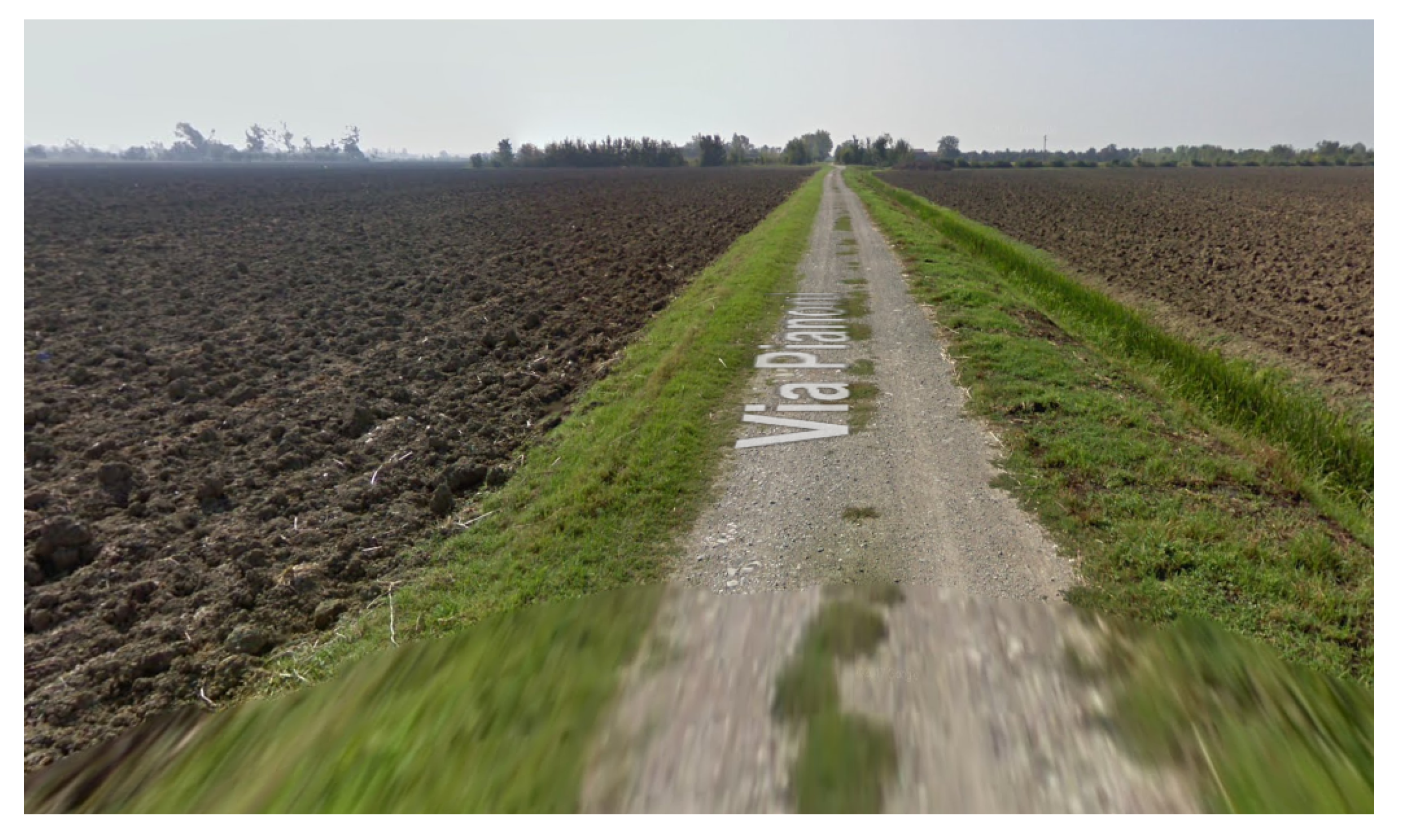
Other experiments have been performed so as to extensively test the algorithm: namely, two more semi-urban tests (i.e., combining urban environment with some highway roads), six additional circuit tests (Figure 9), and two more offroad tests (performed on paths very similar to that of Via Pianoni, see Figure 10). The driver has been required to drive some tests in an aggressive way and some others in a calm way: indeed, one’s perception of aggressiveness is subjective, and difference exists between different tests in which the same person is asked to drive in the same way. These results are collected in the barplot of Figure 21: the figure highlights a net separation between calm and aggressive tests. Furthermore, we can appreciate the differences among tests labeled in the same way. Finally, note that the offroad tests are overall evaluated with positive scores. This is concordant with the considerations done in Section 2.2.3: the aggressive driving features cannot be exaggerated in offroad conditions, thus motivating the importance given to the urban tests, which are indeed much more critical for the considered KPIs.

3.1. Comfort Index Validation through Seat Imu

Finally, in this paragraph we show how the computation of $CI$ through the deck-referenced accelerations is not critical in the comfort level assessment. In the urban and semi-urban experiments previously mentioned, the data coming from the seat IMU described in Section 2 are recorded, and $eVDV=C{I}_{raw}$ is computed according to the procedure detailed in Section 2.1.4. The results are reported in

Table 2. Comfort Index validation, comparison between the observed $eVDV$ at the seat and at the cabin deck.

Test	$\mathit{eVDV}\left[{\displaystyle \frac{\mathit{m}}{{\mathit{s}}^{1.75}}}\right]$
	Deck	Seat
Urban aggressive	$2.13$	$2.78$
Semi-urban aggressive	$1.91$	$2.52$
Semi-urban calm	$1.64$	$2.17$
Urban calm	$1.60$	$2.15$

: as one could expect, the numeric values for the two placements are slightly different. However, the same ranking among the four experiments is obtained, namely, with the urban aggressive test being the less comfortable and the urban calm test being the more comfortable. Eventually, by means of a suitable calibration procedure (Section 2.2.3), the seat $eVDV$ could be scaled so as to obtain a 0–100 scoring, and the tests would be evaluated in a similar way as for the deck IMU.

4. Conclusions

In this research, an algorithm for the real-time estimation of the driving style in agricultural tractors was developed. The algorithm estimates the three key components of the DS, namely, safety, economy, and comfort. The safety estimation module is based upon an experimentally identified safe driving region and evaluates the operator behavior, penalizing the accelerations outside of said region; the economy estimator is instead based upon a longitudinal dynamics model of the vehicle, integrated with an estimation of the road inclination angle so as to guarantee the functionality in a wider variety of conditions. Finally, the comfort assessment is based upon ISO-defined filtering and evaluation procedures. A calibration phase was performed by means of ad-hoc experiments, so as to map the indices onto a 0–100 scoring, which is immediately understandable by the driver and thus more effective. An extensive experimental campaign conducted on different terrain types completes the work, highlighting the effectiveness of the proposed system.

Future research efforts could be directed towards a more complete evaluation algorithm, possibly taking into account other signals or information not considered so far, e.g., the machine payload or the terrain characteristics.

References

- Corno, M.; Furioli, S.; Cesana, P.; Savaresi, S.M. Adaptive Ultrasound-Based Tractor Localization for Semi-Autonomous Vineyard Operations. Agronomy 2021, 11, 287. [Google Scholar] [CrossRef]
- Gupta, C.; Tewari, V.; Ashok Kumar, A.; Shrivastava, P. Automatic tractor slip-draft embedded control system. Comput. Electron. Agric. 2019, 165, 104947. [Google Scholar] [CrossRef]
- Romeo, L.; Petitti, A.; Marani, R.; Milella, A. Internet of Robotic Things in Smart Domains: Applications and Challenges. Sensors 2020, 20, 3355. [Google Scholar] [CrossRef] [PubMed]
- Jaarsma, C.F.; Vries, J.R.D. Agricultural Vehicles and Rural Road Safety: Tackling a Persistent Problem. Traffic Inj. Prev. 2014, 15, 94–101. [Google Scholar] [CrossRef] [PubMed]
- Antunes, S.M.; Cordeiro, C.; Teixeira, H.M. Analysis of fatal accidents with tractors in the Centre of Portugal: Ten years analysis. Forensic Sci. Int. 2018, 287, 74–80. [Google Scholar] [CrossRef]
- Manzoni, V.; Corti, A.; De Luca, P.; Savaresi, S.M. Driving style estimation via inertial measurements. In Proceedings of the 13th International IEEE Conference on Intelligent Transportation Systems, Funchal, Portugal, 19–22 September 2010; pp. 777–782. [Google Scholar]
- Ma, H.; Xie, H.; Huang, D.; Xiong, S. Effects of driving style on the fuel consumption of city buses under different road conditions and vehicle masses. Transp. Res. Part D Transp. Environ. 2015, 41, 205–216. [Google Scholar] [CrossRef]
- Brunetti, J.; D’Ambrogio, W.; Fregolent, A. Analysis of the Vibrations of Operators’ Seats in Agricultural Machinery Using Dynamic Substructuring. Appl. Sci. 2021, 11, 4749. [Google Scholar] [CrossRef]
- Kumar, A.; Mahajan, P.; Mohan, D.; Varghese, M. IT—Information Technology and the Human Interface: Tractor Vibration Severity and Driver Health: A Study from Rural India. J. Agric. Eng. Res. 2001, 80, 313–328. [Google Scholar] [CrossRef]
- Servadio, P.; Marsili, A.; Belfiore, N. Analysis of driving seat vibrations in high forward speed tractors. Biosyst. Eng. 2007, 97, 171–180. [Google Scholar] [CrossRef]
- Jachimczyk, B.; Dziak, D.; Czapla, J.; Damps, P.; Kulesza, W.J. IoT On-Board System for Driving Style Assessment. Sensors 2018, 18, 1233. [Google Scholar] [CrossRef] [Green Version]
- Shope, J.T. Influences on youthful driving behavior and their potential for guiding interventions to reduce crashes. Inj. Prev. 2006, 12, i9–i14. [Google Scholar] [CrossRef] [PubMed]
- Mayhew, D.R.; Simpson, H.M. The safety value of driver education an training. Inj. Prev. 2002, 8, ii3–ii8. [Google Scholar] [PubMed]
- Martinez, C.M.; Heucke, M.; Wang, F.Y.; Gao, B.; Cao, D. Driving Style Recognition for Intelligent Vehicle Control and Advanced Driver Assistance: A Survey. IEEE Trans. Intell. Transp. Syst. 2018, 19, 666–676. [Google Scholar] [CrossRef] [Green Version]
- Fugiglando, U.; Massaro, E.; Santi, P.; Milardo, S.; Abida, K.; Stahlmann, R.; Netter, F.; Ratti, C. Driving Behavior Analysis through CAN Bus Data in an Uncontrolled Environment. IEEE Trans. Intell. Transp. Syst. 2019, 20, 737–748. [Google Scholar] [CrossRef] [Green Version]
- Wang, W.; Xi, J.; Zhao, D. Driving Style Analysis Using Primitive Driving Patterns with Bayesian Nonparametric Approaches. IEEE Trans. Intell. Transp. Syst. 2019, 20, 2986–2998. [Google Scholar] [CrossRef] [Green Version]
- Constantinescu, Z.; Marinoiu, C.; Vladoiu, M. Driving Style Analysis Using Data Mining Techniques. Int. J. Comput. Commun. Control 2010, 5, 654–663. [Google Scholar] [CrossRef]
- Guo, Q.; Zhao, Z.; Shen, P.; Zhan, X.; Li, J. Adaptive optimal control based on driving style recognition for plug-in hybrid electric vehicle. Energy 2019, 186, 115824. [Google Scholar] [CrossRef]
- Bejani, M.M.; Ghatee, M. A context aware system for driving style evaluation by an ensemble learning on smartphone sensors data. Transp. Res. Part C Emerg. Technol. 2018, 89, 303–320. [Google Scholar] [CrossRef]
- Han, W.; Wang, W.; Li, X.; Xi, J. Statistical-based approach for driving style recognition using Bayesian probability with kernel density estimation. IET Intell. Transp. Syst. 2018, 13, 22–30. [Google Scholar] [CrossRef] [Green Version]
- Vaiana, R.; Iuele, T.; Astarita, V.; Caruso, M.V.; Tassitani, A.; Zaffino, C.; Giofré, V.P. Driving Behavior and Traffic Safety: An Acceleration-Based Safety Evaluation Procedure for Smartphones. Mod. Appl. Sci. 2014, 8, 88–96. [Google Scholar] [CrossRef]
- Savaresi, D.; Formentin, S.; Savaresi, S.M. Data-driven mass estimation in continuously variable transmission agricultural tractors. In Proceedings of the 2021 American Control Conference (ACC), New Orleans, LA, USA, 25–28 May 2021; pp. 1529–1534. [Google Scholar]
- Boniolo, I.; Savaresi, S.M. Estimate of the Lean Angle of Motorcycles—Design and Analysis of Systems for Measuring and Estimating the Attitude Parameters of Motorcycles; VDM Publishing: Saarbrücken, Germany, 2010. [Google Scholar]
- Savaresi, D.; Dettù, F.; Formentin, S.; Savaresi, S.M. On the drivability of DC brushless motors with faulty hall sensors during braking maneuvers. In Proceedings of the 2020 IEEE Conference on Control Technology and Applications (CCTA), Montreal, QC, Canada, 24–26 August 2020; pp. 219–224. [Google Scholar]
- Colombo, T.; Panzani, G.; Savaresi, S.M.; Paparo, P. Absolute driving style estimation for ground vehicles. In Proceedings of the 2017 IEEE Conference on Control Technology and Applications (CCTA), Maui, HI, USA, 27–30 August 2017; pp. 2196–2201. [Google Scholar] [CrossRef]
- ISO. ISO 2631-1:1997: Mechanical Vibration and Shock—Evaluation of Human Exposure to Whole-Body Vibration; ISO: Geneva, Switzerland, 1997. [Google Scholar]
- Sim, K.; Lee, H.; Yoon, J.W.; Choi, C.; Hwang, S.H. Effectiveness evaluation of hydro-pneumatic and semi-active cab suspension for the improvement of ride comfort of agricultural tractors. J. Terramech. 2017, 69, 23–32. [Google Scholar] [CrossRef]
- Spelta, C.; Savaresi, S.M.; Previdi, F.; Galli, F.; Tremolada, S. Modeling and identification of vertical dynamics of an agricultural machine. In Proceedings of the 2009 IEEE Control Applications, (CCA) Intelligent Control (ISIC), St. Petersburg, Russia, 8–10 July 2009; pp. 101–106. [Google Scholar]
Figure 1.
The tractor employed in this work, with a detail of the sensor mounting points. (a) Tractor; (b) trailer; (c) dashboard sensor; (d) deck sensor.
Figure 2.
Block scheme of the DS assessment algorithm.
Figure 3.
Ideal and real vehicle speed (and its derivative) in eco (upper plot) and non-eco tests (lower plot). (a) Eco driving test. (b) Non-eco driving test.
Figure 4.
Block scheme of the Eco Index estimation algorithm.
Figure 5.
Longitudinal and lateral accelerations: raw pre-processed signals (left plot) and driver-oriented filtering (right plot). (a) Raw signals. (b) Filtered signals.
Figure 6.
Experimentally identified safe region, for the deck IMU.
Figure 7.
Block schemes representation of the Safety Index estimation algorithm.
Figure 8.
Block schemes representation of the Comfort Index estimation algorithm.
Figure 9.
Circuit considered in the road calibration tests (Argo Terminal, Fabbrico, Italy).
Figure 10.
Gravel track considered in one of the offroad calibration tests (Via Pianoni, Fabbrico, Italy).
Figure 11.
Roll and pitch orientation angles in the circuit and offroad paths. (a) Circuit path. (b) Offroad path.
Figure 12.
Eco Index calibration procedure.
Figure 13.
Distribution of the filtered lateral accelerations in a safe driving test.
Figure 14.
Safety Index calibration procedure.
Figure 15.
Acceleration spectra comparison: deck versus dashboard sensor.
Figure 16.
Comfort Index calibration procedure.
Figure 17.
Path followed in the urban tests.
Figure 18.
Safety Index and g-g plots, for two urban driving tests, an aggressive one (upper plot), and a not-aggressive one (lower plot). (a) Aggressive driving. (b) Calm driving style.
Figure 19.
Eco Index and real/ideal speed profiles, for two urban driving tests, an aggressive one (upper plot), and a not-aggressive one (lower plot). (a) Aggressive driving. (b) Calm driving.
Figure 20.
Comfort Index and power spectral density of the frequency-weighted accelerations , for two urban driving tests, an aggressive one (upper plot), and a not-aggressive one (lower plot). (a) Aggressive driving. (b) Calm driving.
Figure 21.
Safety, Eco, and Comfort Indices evaluated for a variety of tests. The label AGG is used to denote aggressive driving tests, where as the label CALM is used to denote calm driving tests.