1. Introduction
According to data from the Pan-European Common Bird Monitoring Scheme (PECBMS) [
1], farmland birds have suffered a significant population decline of over 50% on average over the last 40 years. One of the main drivers of the sharp decline in bird populations has been agricultural intensification, which has led to global biodiversity loss [
1]. One of the most affected groups is steppe birds that depend on the habitats where agricultural activities occur, being very sensitive to the degradation of these environments.
The loss of fallow land has been linked to the decline of steppe bird populations in Spain, [
2], because fallow land (agricultural land left unsown to allow the recovery of soil nutrients) is vital, among other things, for the feeding and maintenance of the species. For this reason, traditional extensive fallow management is considered beneficial for improving biodiversity conservation, especially steppe birds, in agricultural environments.
Since 1960, the European Commission (EC) has aimed to provide a harmonized framework for agriculture through the CAP by defining European cooperation policies and managing support to enforce these rules. In addition, the EC has built a shared context for all its members by using the numerous regulations to achieve a coherent framework for the CAP development [
3] with the applicability of the latest technologies. Tarjuelo et al. [
4] propose a strategy to reconcile agriculture and biodiversity conservation, based on the recovery of fallow land through CAP, to guarantee and conserve the future of steppe birds.
Farmers were not allowed support until the 2014-2020 CAP period, provided they met three measures: maintaining permanent pasture, growing a minimum of three different crops and establishing landscape features considered essential for biodiversity on 5% of the farmland [
5].
The new CAP, therefore, aims to promote the recovery of fallow land and thus also promote the recovery of steppe birds, which have their feeding and breeding grounds in cereal crops. Modifying certain traditional cultivation practices can lead to improved feeding and breeding conditions for these species and thus contribute to improving their population and biodiversity. The Autonomous Community of the Region of Murcia (CARM) aid line for the protection of steppe birds aims to achieve this and sets out obligations associated with the aid to use medium or long-cycle cereal varieties (wheat, spelt, barley, rye, oats and triticale) for sowing and not to harvest before 15 July.
Regulation 1306/2013 [
6] is the most recent CAP financing, management, and monitoring law. It formed the basis for the beginning of the regulation of the uses of new technologies, especially remote sensing: Sentinels satellites, unmanned aerial vehicles (UAV), and georeferenced photographs (Regulation (EU) 2018/746 [
7]).
Remote sensing has been incorporated into the agricultural sector as a helpful tool for tracking and monitoring activities such as crop production, land use monitoring or environmental protection [
8,
9]. The last challenge is its incorporation as an essential tool in the CAP. The CAP wants to take advantage of the new Earth Observation (EO) philosophy the European Space Agency (ESA) is developing in the 21st Century. Copernicus Programme (CP), devised by ESA, aims to provide accurate, up-to-date and easily accessible information to improve environmental management and understand and mitigate the effects of climate change.
Some studies are concerned with analyzing the potential of Sentinel-1 (S1) data for assessing different soil, and cereal parameters, such as the one proposed by Bousbih et al. [
10]. Other works conclude that the synergistic use of radar and optical data for crop classification generates better information and thus increases classification accuracy compared to optical-only classification [
11].
The first remote sensing methodology used to study vegetation has been the opportunity to perform various operations with the bands of satellite images, where the result can be converted into a spectral index. The first and most used index is the Normalized Difference Vegetation Index (NDVI) [
12,
13]. The NDVI is an indicator of the greenness of the biomass [
14]. The NDVI has been used as: Tool for wheat yield estimation [
15], time series [
16], and prediction model [
17].
The Data Cube (DC) Concept is a data cube that describes a multi-dimensional array of values of n-dimensions. This concept was begun used with hyperspectral images in the 90s. The irregular time series cube (ITSC) is a data cube in which data are generated with varying time intervals per spectral index. The ITSC are created from optical images: Landsat [
18], MODIS [
19], Sentinel-2 (S2) and Sentinel-3 [
20] due to cloud cover. However, the use of S1 images has allowed to generation time series cube (TSC), a series of values of a quantity obtained at successive times, often with equal intervals between them [
21]. The use of the ITSC and TSC are ways to visualize and understand a cartographic time series quickly.
The use of the DC has increased due to the development of computing, the cloud infrastructures philosophy, and the Analysis-Ready Data (ARD) products. In compliance with operational standards established by the International Organization for Standardization (ISO) and the Open Geospatial Consortium (OGC), data cubes belong to the category of coverages. The OGC Community Practice has defined such a data cube as “established based on a Coverage with a specific grid system for geospatial data with at least one dimension of the spatial or temporal definition” [
22,
23]. The ARD is then fundamental to the EO data cube, which integrates this data into one logical array multi-temporal thematic analysis. The DC input on machine learning [
24,
25] allows for generating crop modeling [
26]. In this work, the inputs to the generated DCs were multitemporal S1 and S2 images and associated third-level products, such as polarization or vegetation indices, as well as digital elevation model or land use data.
This work aimed to develop a methodology to establish whether applicants for aid for the protection of steppe birds complied with the commitments established in this aid. To this end, following the principles of CAP monitoring, use was to be made of the enormous amount of data provided by the Copernicus Programme through the S1 and S2 ground monitoring missions. In addition, monitoring had to be carried out for all the plots assigned to the aid continuously over time. For each plot, a light traffic color had to be established, whereby red indicated that the commitment was not being fulfilled, green that it was, and yellow that it was impossible to make a clear judgment. Two methodologies were defined and developed in parallel, the results of which were compared to assess which offered the better solution. The first methodology presented a more traditional approach based on remote sensing and finding a biophysical index to obtain an optimal solution. The second methodology was based on Machine Learning and aimed to generate a model that would offer a correct solution with good metrics.
2. Study Area
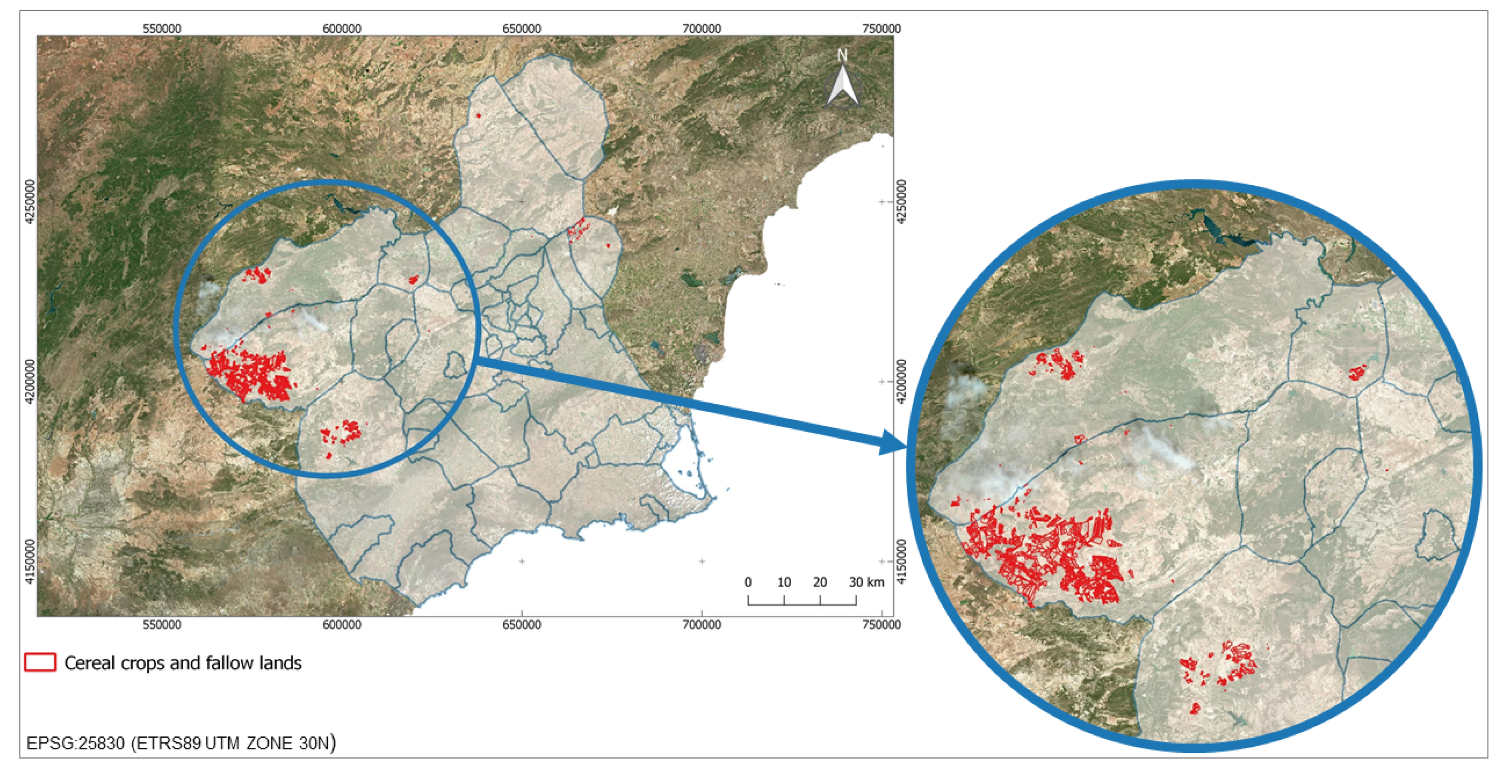
The study area corresponds to the areas where farmers have applied for aid in the CARM. The different plots are located in the zone of the southwest and plateau of Murcia Region. Cereal land cover (wheat, barley, oats) and fallow and plowed soils. The Murcia Region is characterized by warm temperatures almost all year round. According to the distribution of average temperatures in the region, they exceed 17 C in the Murcia city area, the Abanilla-Fortuna basin, and the coast reaching 20 C around Aguilas town. In the interior, it descends to 16 C, 14–16 C in the Altiplano, and 12 C in the Northwest.
Altitude is another factor that increases temperature variations on a local scale, reaching even lower values in the highest areas of Northwest Murcia. The annual thermal amplitudes are 12–13
C on the coast, 14–16
C in depressions and interior valleys to rise to 17
C in the Altiplano. The average rainfall of the basin can be estimated at 375 mm per year [
27], 472 mm at the head, and 317 mm at the bottom.
Figure 1 shows a map indicating the study area location of this work.
Finally, the height of the cereals cultivated in the study area does not exceed 50 cm at the point of greatest vegetative development, which is a crucial characteristic to take into account.
3. Materials
The materials used in this work come from various sources, such as vector and alphanumeric information from help applications, satellite images or data on agricultural land use, together with information on the terrain orography of the study area.
For the development of this work, a proprietary tool based on free software was implemented. This tool was implemented in the Python programming language. It used libraries such as rasterio or geopandas for GIS data processing, and for the functionality linked to Machine Learning, it used scikit-learn. A PostgreSQL database with the PostGIS spatial extension for data storage. The requests library and the Copernicus Open Access API Hub were combined to access the satellite image repository.
Finally, the tool was deployed by an in-house server with Windows 2016 Server as the operating system, 64 GB RAM, 4TB hard drive, and an NVIDIA RXT2080Ti graphics card.
3.1. Aid Declarations Data
The information related to the aid applications is included in the Aid Management application of the Regional Ministry of Water, Agriculture, Livestock, Fisheries, and Environment of the Region of Murcia.
The information we can find in this dataset is identifying the agricultural parcel requesting the aid, the code of the aid requested, and the enclosure’s geometry. The reference system of the vector data is ETRS89 (EPSG:25830).
For the campaign under study, 2019, included in the study area, 1466 applications were submitted, with 9690 hectares. Out of the total number of applications, a reduced number is selected to elaborate the ground-truth matrix, which will be used later for learning the model.
3.2. Remote Sensing Data
The satellite images used to carry out this work belong to ESA’s Copernicus Programme [
28] and, more specifically, to the missions focused on terrestrial monitoring, such as S1 and S2. While S1 provides radar images, S2 provides optical images.
The main instrument of S1 is a synthetic aperture radar (SAR) in C-band. The main advantage of this type of satellite is that it can provide images regardless of whether it is day or night and in any weather conditions. The reference system in which these images are provided initially is EPSG:4326. Relative orbits 8 (slices 24 and 25) and 103 (slices 2 and 3) provide coverage of the study area. The product used from the S1 was the Ground Range Detected (GRD).
We did not use the native images provided in the ESA repository for this work, but we carried out a processing [
29] for further analysis. This processing applies a series of standard corrections and consists of applying the following seven steps:
From the last item in the above list, we get the VV and VH polarized backscatter
0_VV and
0_VH, in decibels (dB) [
30,
31,
32,
33,
34] with a damping value of 1 and a kernel size of 7 × 7 to minimize radar speckle in the pictures.
The VV and VH channels are used for the characteristic matrix and the VV+VH and VV-VH dual polarizations.
S2 carries a Multispectral Instrument (MSI), defined as a high resolution, wide swath multispectral imaging system operating in 13 spectral bands at multiple spatial resolutions. The product type used is S2MSI2A, whose main features are level 2A processing, orthorectified and UTM geocoding, BOA, and multispectral reflectance [
35]. All elements of this time series had 0% cloud cover over the study area and were provided in the EPSG:32630 reference system. The S2 scene providing coverage for the study area is T30SWH.
All the bands offered in the S2 images were used to carry out this work. The
Table 1 shows detailed technical information about these bands:
Third-level products derived from S2 imagery were also used for this work. These products are the vegetation indices NDVI [
13], GNDVI [
36], SAVI [
37], and OSAVI [
31].
In addition, we also used images from a unmanned aerial vehicle (UAV).
3.3. External Data
The Geographic Information System of Agricultural Parcels, SIGPAC [
38], allows the geographic identification of the parcels declared by farmers and livestock farmers in any aid scheme related to the area cultivated or used by livestock. In addition to the above information, SIGPAC provides the declared land use for each declared agricultural enclosure. At a general level, the SIGPAC distinguishes 30 different agricultural land uses. For this work, we did not have information on the specific crop of each of the studies included in the study area but rather a typology in which they could be included.
The data on the orography of the terrain included in the study area is obtained through the digital elevation model (DEM) provided by the National Center for Geographic Information (CNIG) [
39]. The digital model used in this work has a grid pitch of 5 m and is presented in the ETRS89 geodetic reference system.
3.4. Field Data Campaign
The field campaigns were designed based on the information provided by the CARM. The plots were documented by survey in Survey123, filled with a Samsung Galaxy Ta2 Tablet, and photographed with Canon EOS 70D camera installed on a tripod. In a random way and based on the plot with the aid applications provided by the CARM, it was decided in which plots the field radiometry would be carried out with an Ocean Optics radiometer. Through these campaigns, a ground-truth matrix was created.
4. Methods
The work we are concerned with in this paper was approached through two different methodologies, the results of which will be confronted at the end of the paper. These methodologies were developed in parallel and aimed at determining whether aid declarants complied with their obligations.
The first methodology, BirdsEO, had a more traditional approach as it used earth observation techniques based on satellite imagery or derived products. The objective was to obtain an index derived from these satellite images to discern whether respondents complied with their obligations.
The second methodology, called BirdsML, presented a somewhat more contemporary approach, as it used Machine Learning techniques in combination with satellite imagery from Sentinel missions 1 and 2. The objective of this methodology was to obtain a Machine Learning-based model that would predict, based on probabilities, whether or not aid applicants were compliant.
The project has a duration of three years. It began on 1 July 2019. The planning was dynamic, and it changed with the evolution of the project. The activities schedule can be consulted in
Table A1.
4.1. BirdsEO
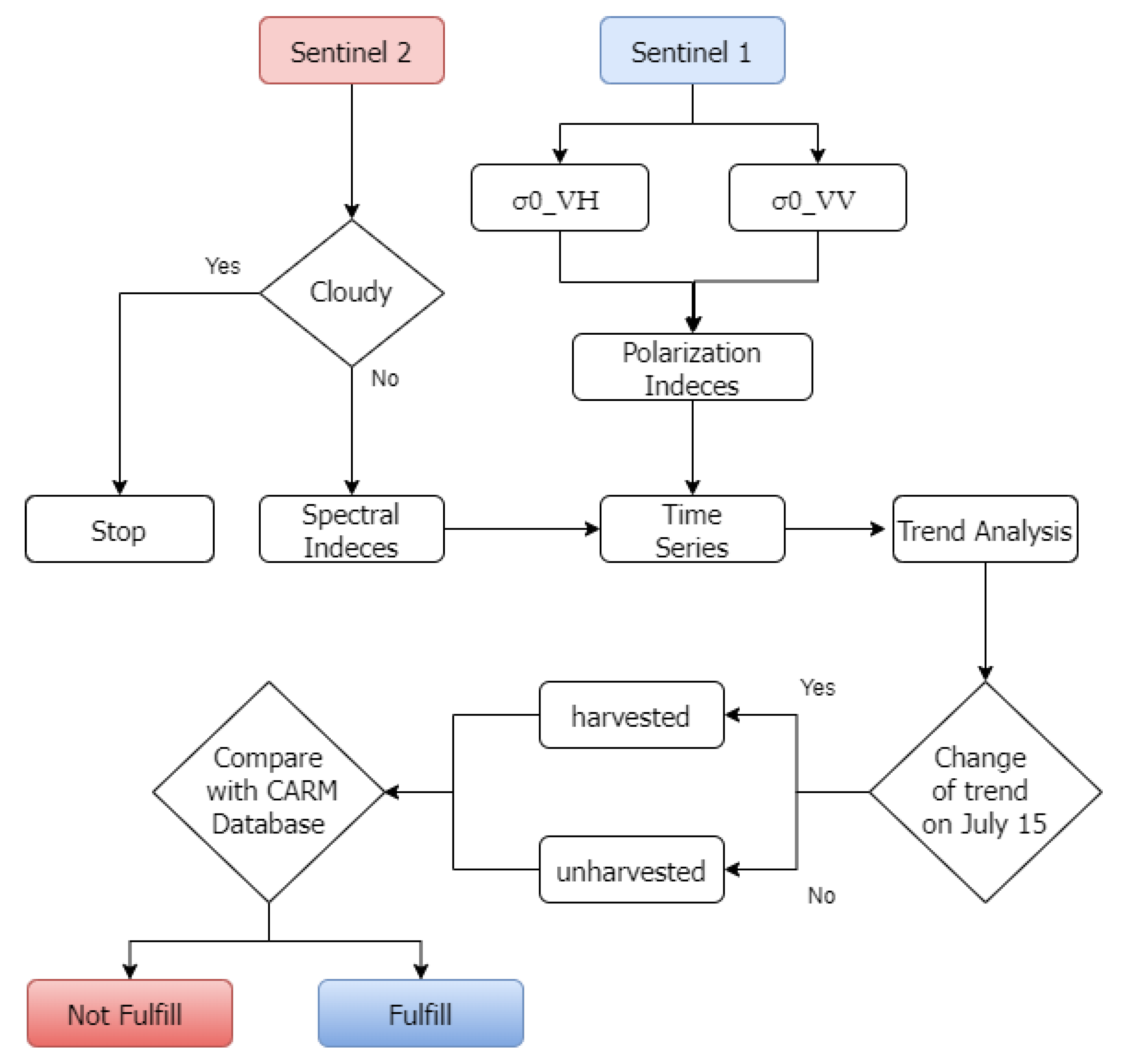
The project was planned as a decision tree, as shown in
Figure 2, which inputs were the images and outputs were the plots harvested before or after July 15. Decisions would be made based on thresholds of spectral and polarization indices. First, we work with the satellite images; for S2, we check the cloud cover and generate the spectral indices and, in the same way, for S1, we develop the derived products and their corresponding polarised indices. After this step, the previous results are incorporated into the time series. Then, a trend analysis of the time series is carried out to check that there is a drop in the indices as the plot is harvested [
17]. Finally, because the images can only identify which plots are harvested or not, it is necessary to identify which farmers have applied for aid; for this reason, it is needed to compare with the CARM database to know which applicants do or do not meet the aid requirements.
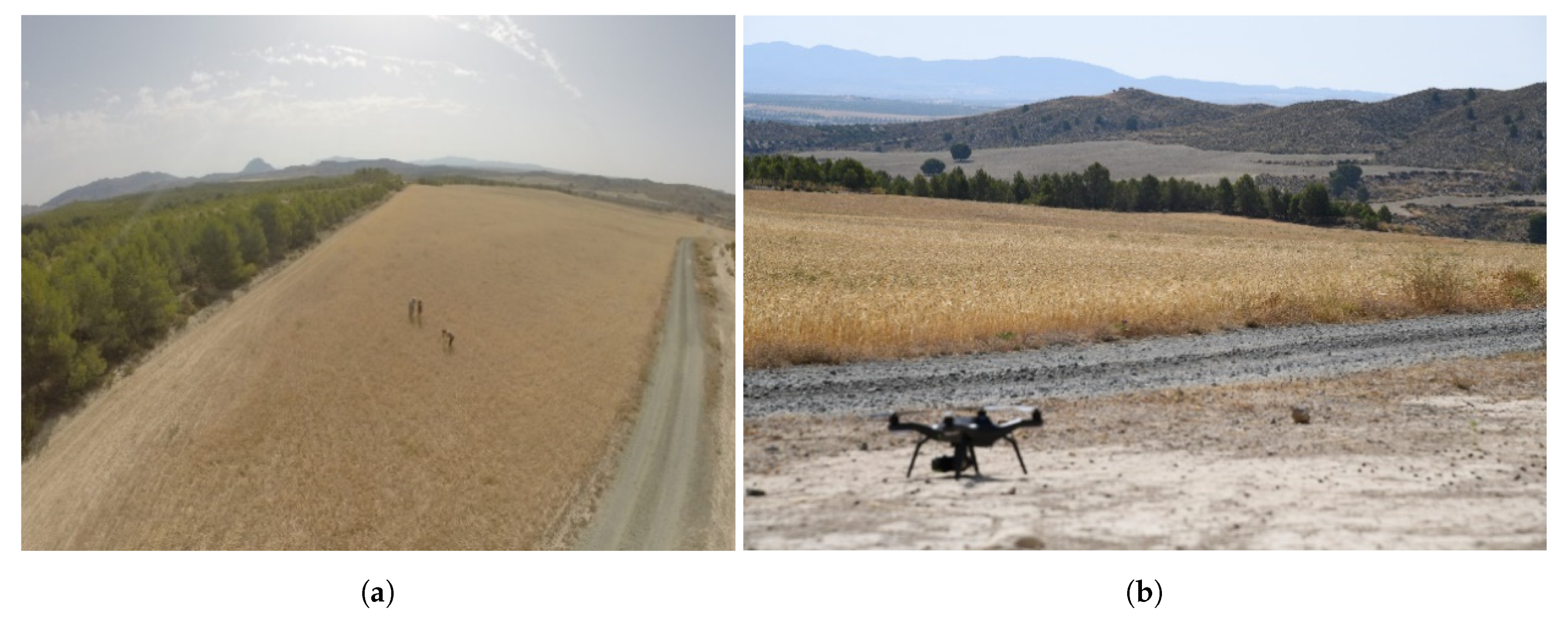
The first step was to make those responsible in the Ministry of Agriculture of the CARM and the farmers understand the problems with protecting steppe birds in the Region of Murcia and what needs to be covered. The field data campaigns were selected from aid requested GIS, and they have three different aims: radiometry campaign, UAV campaign (
Figure 3), and getting data about crop type and phenology using Survey123.
The radiometry campaigns aimed to know the surface’s spectral response through reflectance measures. The reflectance (
R(
)) was obtained according to:
Surface radiance (
(
)), surface white reference radiance (
(
)), and correction factor white (
(
)). The continuous spectra are transformed to discrete spectra according to UAV and S2 bands:
Spectral response functions of S2 and UAV bands (()), cover reflectance (R()), and cover reflectance of S2 and UAV bands ().
The UAV flights were simultaneous to the radiometry campaigns above the same crop areas. Acquired data were processed using Pix4Dmapper (Pix4D SA, Cheseaux—Lausanne, Switzerland), where image calibration, point cloud densification, and ortho-photomosaics (in WGS 84 UTM Zone 30 coordinate system) were calculated from each of the datasets [
40].
The following biophysical indices were generated using the red, green and blue bands of the S2 images: Normalized Green Red Difference Index (NGRDI) [
40,
41], Green Leaf Index (GLI) [
42], Red Green Blue Vegetation Index (RGBVI) [
43], Visible Atmospherically Resistant Index (VARI) [
44] and Triangular Greenness Index (TGI) [
45].
The Sentinels images were downloaded weekly from EarthExplorer ESA Hub Copernicus. The S2 images were converted to 10 m spatial resolution using ESA free software, the Sentinel Application Platform (SNAP) [
46].
Each image’s bands were resampled to 10 m using SNAP [
47] and calculated the following spectral indices. However, there is a wide variety of them [
44]: Normalized Difference Vegetation Index (NDVI), Green Difference Vegetation Index (GDVI), Green Normalized Difference Normalized Vegetation Index (GNDVI), Normalized difference near-infrared/shortwave infrared Normalized Burn Ratio (NBR) and Normalized Difference Infrared Index (NDII) [
48]. Other spectral indices are proposed based on inverse reflectance differences, such as Anthocyanin Reflectance Index (ARI) or Carotenoid Reflectance Index (CRI550) [
49]. However, most indices are based on reflectance in more than three bands. Some indices, such as the Soil Adjusted Vegetation Index (SAVI) [
50] and Chlorophyll Absorption Ratio Index (CARI) [
51], are based on a transformation technique to minimize the influence of soil brightness or the effects of non-photosynthetic materials, and they have very complex forms. In addition, integrated indexes such as the Transformed Chlorophyll Absorption Ratio (TCARI) and Optimized Soil Adjusted Vegetation Index (OSAVI) were taken into account for this work [
52]. The spectral index of each date was exported to ENVI format. In ENVI v4.8, irregular time series spectral indices cube (ITSIC) was generated.
The S1 images used in this project were Ground Range Detected (GRD) Interferometric Wide Swath (IW) products. The radar images were projected onto a standard 10-m grid in GRD output using SNAP-free software from the ESA.
The polarization indices were calculated [
30]: Polarization Ratio Index (PRI), Normalize Difference Polarization Index (NDPI), and Polarization Index (PI). Finally, it is exported to ENVI v4.8 format, and a time series polarisation index cube (TSPIC) was generated.
4.2. BirdsML
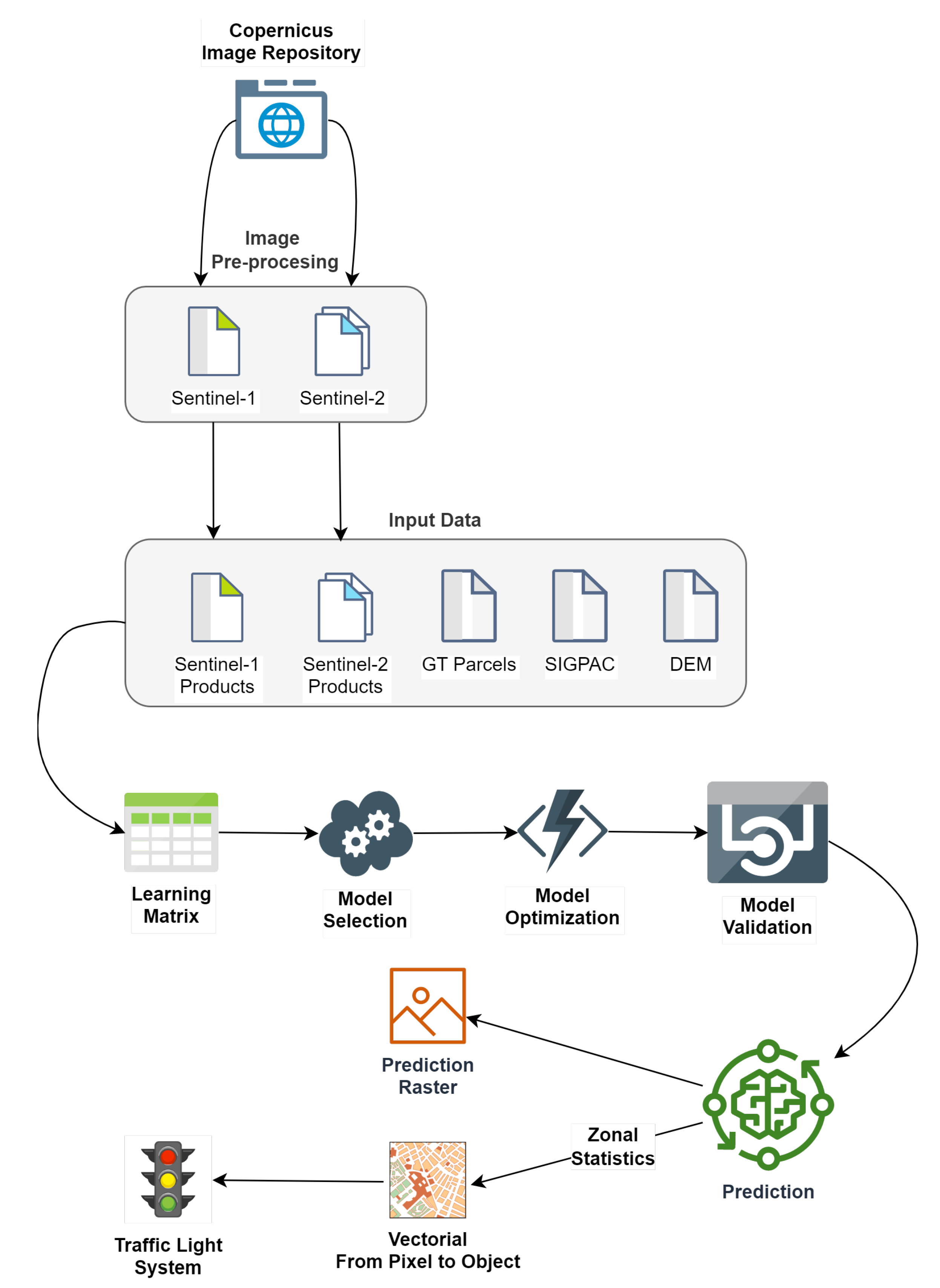
Figure 4 shows a summary of the workflow of the methodology defined to carry out this work:
In short, the objective of this work was to develop a methodology that, through satellite data and other data from different sources and the use of Machine Learning techniques, would make it possible to check whether the aid applicants complied with the obligations undertaken. Following the CAP monitoring process guidelines, the final result was based on a traffic light system, with red indicating that the commitment was not fulfilled, green that it was fulfilled and yellow that it is impossible to give a clear verdict.
4.2.1. Sentinel Repository
Using the Copernicus Hub API, a process was implemented that established a connection with the Hub and obtained the S1 and S2 images for a specific date after performing the appropriate queries.
This same process was in charge of preprocessing the Sentinel images. On the one hand, on the S1 images, applying the transformations indicated in that section. On the other hand, it generated the third-level products derived from the S2 images, indicated in the section with the same name.
Once the preprocessed Sentinel images were available, a cropping operation was applied to adjust them to the study area. Other reprojection operations were applied so that all the input data had the same reference system. In this case, the reference system selected was EPSG:32630.
4.2.2. Input Data
In addition to the preprocessed Sentinel images, the implemented methodology used information related to the ground-truth plot, agricultural land use according to SIGPAC, and the digital elevation model.
In this part, the implemented process performed tasks related to the standardization of the input data in order to make their combination possible. In this way, rasterization was applied to the true-land parcel. The agricultural use information performed a spatial cross-referencing with the true-land parcel and subsequent rasterization.
Once all the input data were in raster format, proceed with the resampling. They all had a spatial resolution of 10 m and, finally, with a reprojection to the EPSG:32630 reference system.
4.2.3. Ground-Truth Data
Theground-truth data used contained elements of two different classes. Class 1 indicates that the obligation to help was fulfilled, and class 99 indicates that it was not. The samples were generated through information obtained from field visits.
As a result, a sample of 43,096 pixels was obtained, which was distributed as shown in the
Table 2:
For the Fulfill class, utilizing field visits, a series of plots were selected that were going to be cultivated with medium or long-cycle cereals and that had not applied for the aid associated with the protection of steppe birds. In this way, it was possible to generate ground-truth information that would not subsequently have to be predicted by the model, thus avoiding, as far as possible, over-fitting and favoring better generalization by the model, which translates into more accurate predictions. They were incorporated into the ground-truth matrix as polygons.
For the Not Fulfill class, on S2 images, a series of polygons were digitized randomly over areas where no cereals of the type included in the aid obligations were grown. These polygons were located on areas with a similar appearance to the crops they intended to identify and on areas with a completely different appearance.
The spatial resolution of the ground truth matrix was the same as that of the input data (
Section 4.2.2) so that each pixel was 10 × 10 m in size.
Concerning the Sentinel images, as the objective was to infer whether the aid declarations had complied with the requested aid obligations as of 15 July 2019 crop year, the implemented process generated a time series composed of 8 images between March and July 2019.
At this point, to discern how each input data contributed to the model’s performance, the implemented process generated different learning matrices by combining these input data. In addition to the input data indicated in the previous section, the developed process incorporated, in the ground-truth matrix, features related to date and location. In this way, the following datasets were generated:
Table 3 specifies the features and the number of bands that made up each of the datasets generated:
As a method of selecting training and test items, the traditional percentage division, whereby a percentage, e.g., 80%, of the original dataset, goes to training and the rest to testing, was discarded. Instead, K-Fold cross-validation was used to adjust and validate the model [
53], with k = 5. This method, for K times, mixes the dataset randomly and then divides the dataset into K groups. One of the groups is taken as test data set, and the remaining as training data. With the division done, it fits a model on the training dataset and evaluates it with the test dataset. Once finished, the score of the selected metrics is recorded, and the model is discarded. The final performance of the proposed model will be the average of the K times the process has been run. Thus, we have a less optimistic estimate of the model’s performance.
Finally, data normalization operations and balancing of the ground-truth matrix [
54] were applied to ensure that the evaluated models competed on an equal footing.
4.2.4. Model Selection
The implemented process evaluated the performance of several Machine Learning classification models, including the classic KNN, Decision Tree (CART), Extra Trees (EXT), Random Forest (RF), Bagging (BG), or more novel XGBoost [
55] (XGB), and LightGBM [
56] (LGBM).
The dataset used for this part of the process was the one with the most features, labeled S2-S1-COOR-OTHER.
The approach for developing this work was to have simple models initially and then sophisticate the model with the best initial performance. For this initial step, it was decided to use the baseline of all the selected models to evaluate their performance. These baseline models were created with the minimum possible definition and using the indispensable parameters for their creation. The default definition established by the scikit-learn library was used for all of them. This section aimed to contextualize and understand the datasets’ characteristics and the possible potential of the selected models with the created datasets. K-Fold type cross-validation was used for the validation of the models, with k = 5, and the selected metrics were Accuracy (ACC),Kappa, Precision, Recall, F1, and Area under the ROC Curve (ROC-AUC Curve) [
57].
4.2.5. Model Optimization
Once the model with the best performance was selected, it was optimized. For this purpose, many hyperparameters with a wide range of possible values were selected. Again, cross-validation was used for the combination of values. The hyperparameters selected for optimization were the number of estimators, maximum number of features, maximum depth, number of elements per leaf, or class weight. The Grid Search method was used as an optimization method, which evaluates the model’s performance for every possible combination that can be given, and finally, the combination with the set of values that offers the best performance.
4.2.6. Model Validation
Again, cross-validation was the technique selected to validate the optimized model. The metrics generated were the same as those in the Model Selection section. In addition, the confusion matrix was generated, which, although not a metric in itself, is beneficial for understanding the model’s performance. Learning and model validation curves were also generated, along with a list of the importance of different features in making a prediction.
4.2.7. Prediction
In the final phase, the implemented process predicted the total surface of the study area at the pixel level. It generated a raster in which, for each pixel, the predicted class and the probabilities of belonging to the two existing classes were recorded.
On the other hand, to make a definitive judgment as to whether or not the declarant complied with the aid obligations, based on the traffic light system, it was necessary to move from a classification by pixel to a classification by an object, at the parcel level.
For this purpose, the algorithm obtained different zonal statistics between the raster resulting from the Machine Learning classification and the parcel with the aid declarations. At this point, generic statistics were stored, such as the mean, standard deviation, number of pixels or majority, and other custom-created ones, such as the number of pixels per class and the average probability of the prediction for each class.
Given the zonal statistics of the previous paragraph, to eliminate the influence of non-target items found at the boundaries of the plots, an adjustment was made to analyze the results obtained, excluding the pixels on the perimeter of the enclosure. Once these pixels were excluded, the same statistical information was generated as in the previous paragraph.
In short, this part of the methodology was used to generate many parameters to infer whether or not an applicant complied with the requested aid obligations, regardless of the metrics that can be extracted from the models.
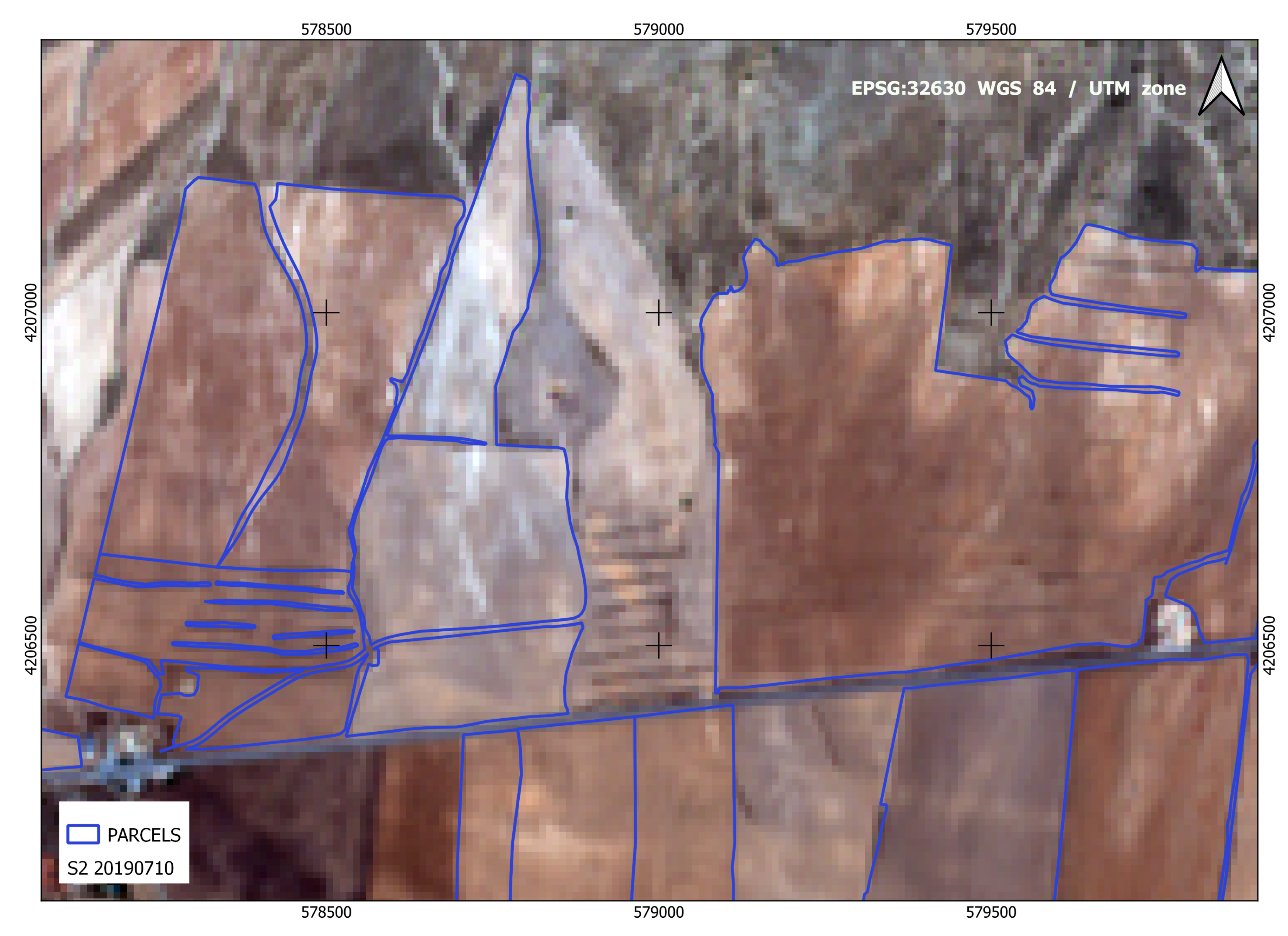
Figure 5 shows, for a given part of the study area, the land use on a date close to 15 July 2019, and the plots applied for steppe bird protection aid. The orthoimage corresponds to a true-color composition from the S2 image of 10 July 2019.
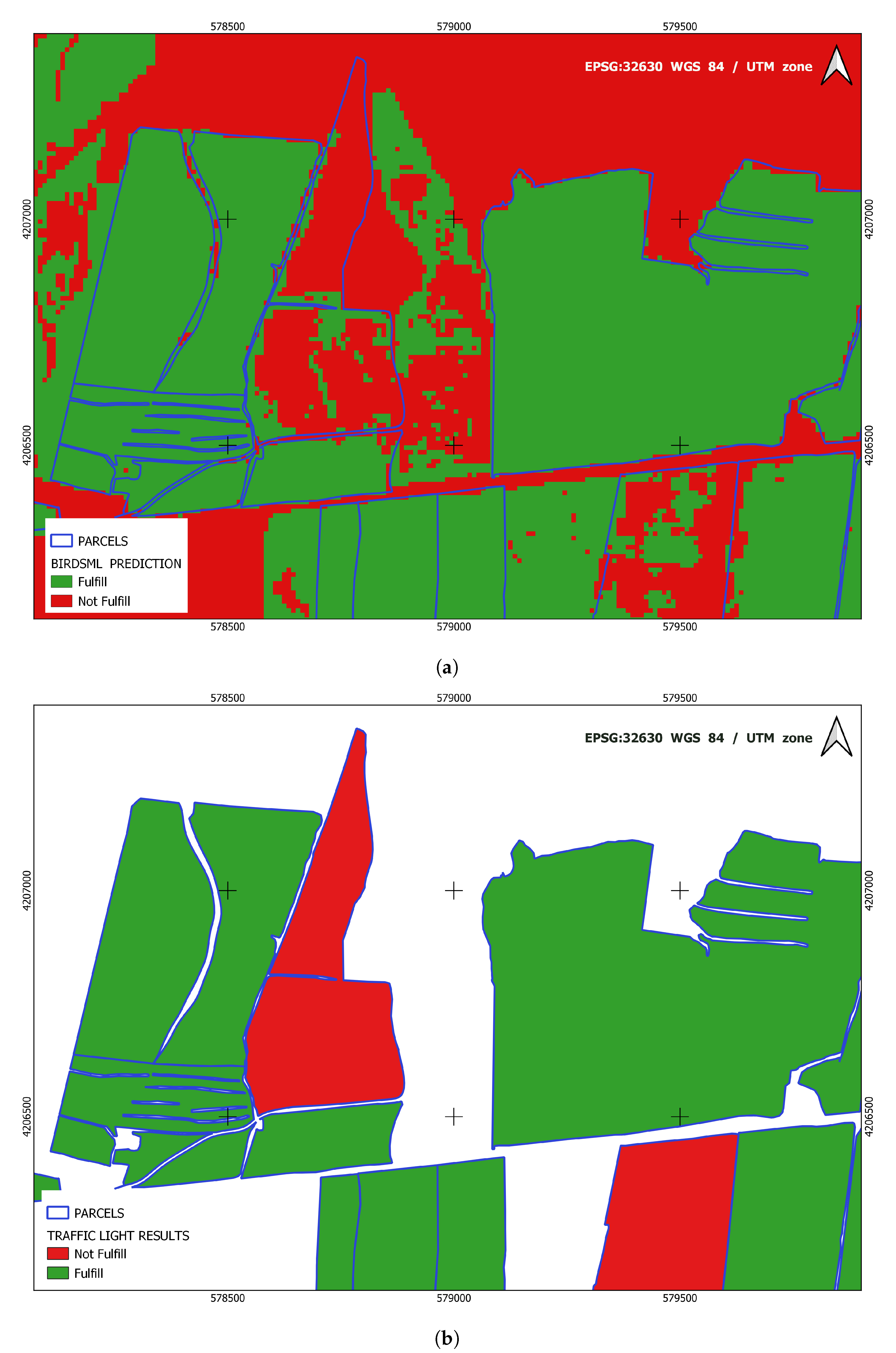
Figure 6a shows the prediction performed by BirdsML for the above area.
Figure 6b shows the results in the form of a traffic light once the classification at the object level is obtained from the classification per pixel for each of the plots. To arrive at this object-level classification, the pixels of the different classes are counted, excluding those on the perimeter of the plots. To minimize the aids awarded when the obligations are not met, a threshold of 70% is set for the parcel to be marked as fulfilled.
5. Results
5.1. BirdsEO
In the first stage, the field data allowed the construction of a spectral library. Thanks to using the ArcGIS Survey123 ESRI’s forms-based tool for creating, sharing and analyzing surveys [
58]. In this way, it has been possible to generate a library where, for each point, all the information acquired during the different campaigns is visualized and thus obtain a cube of irregular time series field data (ITSFDC). The ITSFDCs are converted to Google Earth files to be visualized and located quickly and easily on any platform and computer.
The high spatial resolution of UAVs, in this case, is not a reasonable solution since it requires a high number of flights and the processing of large amounts of files due to the large extension of the study area.
A hyperspectral image is when there is an image of one wavelength in each layer for a specific date. The ITSC was generated per each spectral index in several files because its size was too large and could not be parsed because the pilot plot was scattered east of CARM.
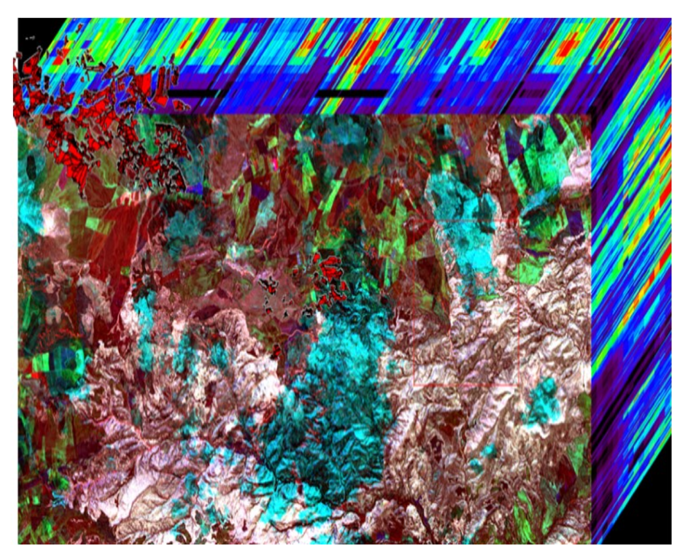
Figure 7 illustrates a 3D cube of a hyper-temporal image as each layer corresponds to a different date of the same variable.
Because the philosophy of the work is to study the trend and to see how the images evolve before and after 15 July, an image before this deadline and one immediately after it had to be available. In the trend analysis for a specific date, the information before and after this date cannot be missing. The image immediately before 15 July was discarded because it had cloud cover, as shown in
Figure 8. It was impossible to analyze what type of crop existed in each plot and its state of harvest.
The time series cubes 0_VV(dB) and 0_VH(dB), as well as the corresponding polarisation index cube (TSPIC), were generated. A suitable pixel was selected in each plot and generated its time series. The radar images obtained by the Sentinel 1A and 1B satellites have a periodicity or revisit for six days. In 2020, there is an image on 12 July and another on July 18 of the study area. The last visit to the field was made on July 16, ending the field campaign and understanding that the situation observed on that day would be the same as that observed by the satellite on 18 July.
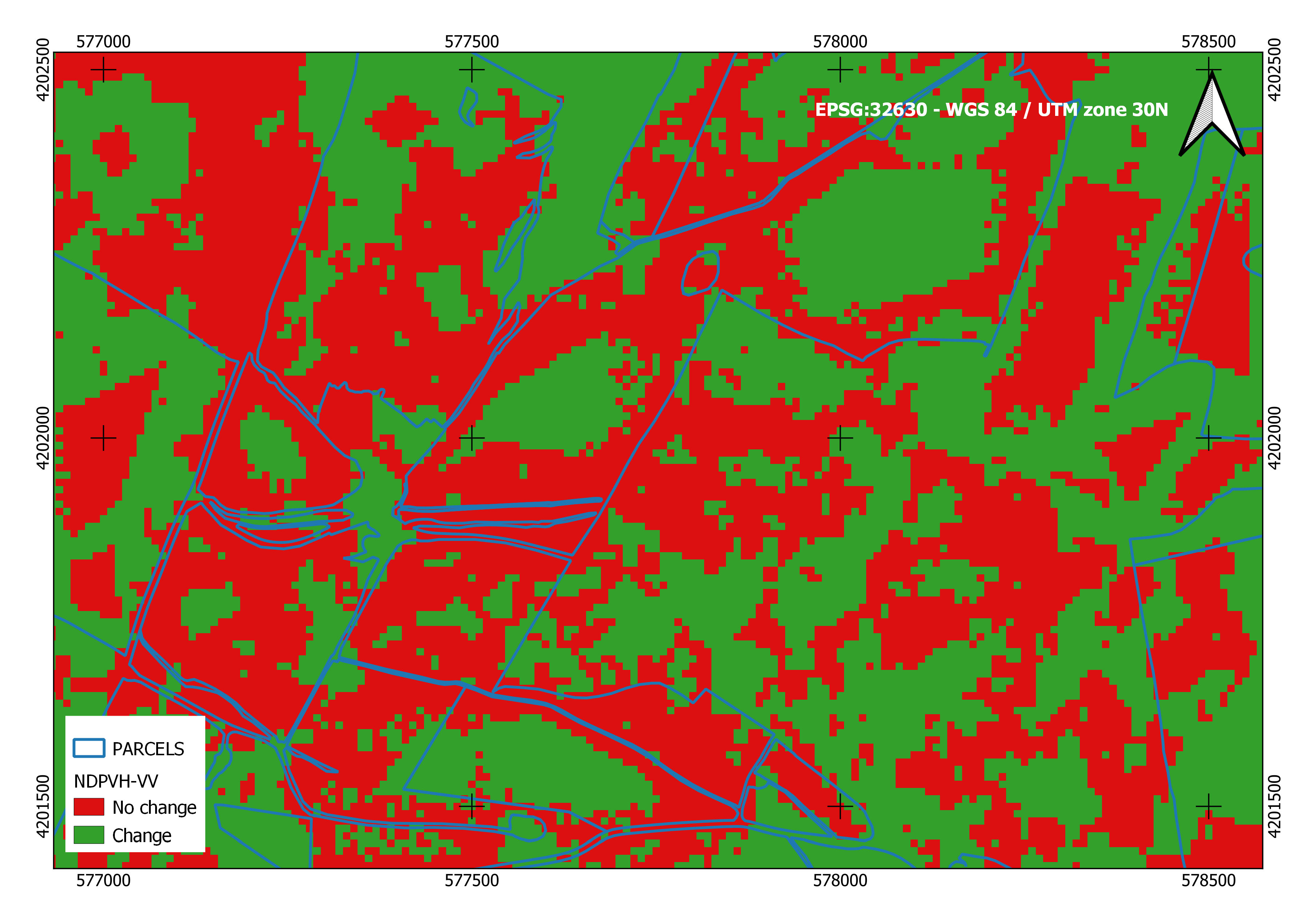
A first comparative analysis of the NDPVH-VV values of 12 and 18 July shows apparent differences between both dates. These differences are observed in a grey range map of the temporal difference map
(NDPVH-VV) (
Figure 9), that is, the difference between NDPVH-VV (After 15 July = 18 July) and NDPVH-VV (Before 15 July). July = 12 July). In the difference map
(NDPVH-VV), we obtain positive values for the areas that do not change and negative values for the areas that change, as observed in the time series of the areas in which the field monitoring has been carried out:
(NDPVH-VV) = NDPVH-VV(After 15 July)-NDPVH-VV (Before 15 July)
(NDPVH-VV) > 0 → No change (red) Not harvested
(NDPVH-VV) < 0 → Change (green) Harvested
Figure 9 shows that there are positive and negative values in the same plot. This is because the slope and plant height influence the radar response, so there are no negative pixels in plots with mostly positive pixels and vice versa.
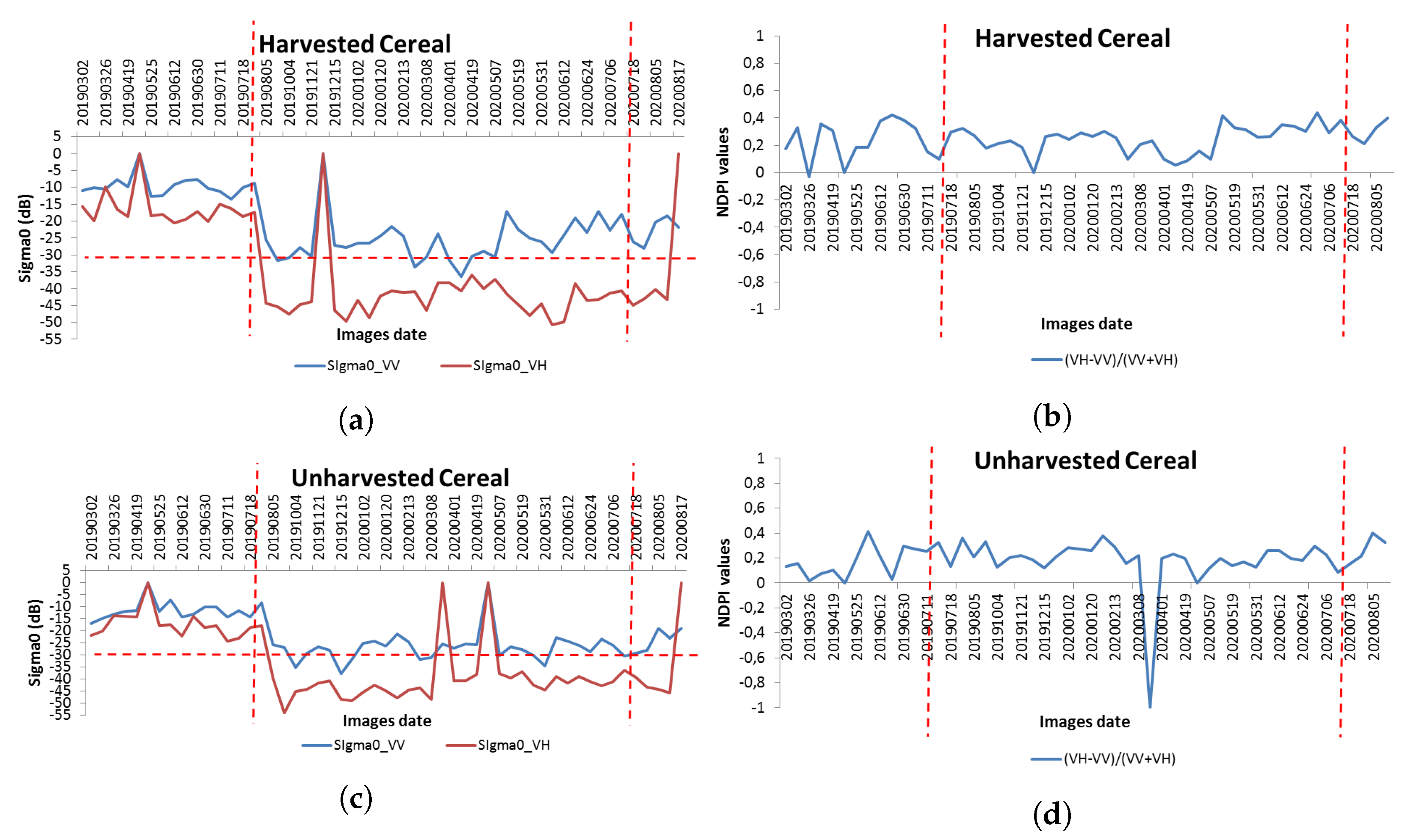
Figure 10 shows the temporal evolution of
0_VV of a harvested plot (a) and a non-harvested plot (c), together with the temporal evolution of the NDPI, subfigures b and d, where it can be seen that on the dates when harvesting takes place (before July 15) the slope tends to be ascending and then descending.
If we focus the analysis within the plots, we observe a corresponding heterogeneity of values of (NDPVH-VV). This heterogeneity is due to the radar signal and the Earth’s surface. The first factor is the terrain relief, and the second is the scattering mechanisms of the radar signal on vegetation.
The approach of developing a methodology that would allow an index to be obtained from traditional techniques using images in the radar and optical range presented several complications: in the optical range due to cloud cover and the radar range due to the slope of the terrain and the height of the crop. For these reasons, all results obtained by this methodology were considered inconclusive.
5.2. BirdsML
In this section, the metrics analyzed by each classifier and the results obtained by the selected model for each dataset generated will be discussed in detail.
5.2.1. Best Model Selection
Once the ground-truth matrix was generated, the first task of the implemented tool was to select the best performing Machine Learning model for the dataset with the most features (S2-S1-COOR-OTHER), with its normalized or standardized data, balanced and with the baseline definition of each of the models. The models selected for evaluation could be divided between the classics, such as KNN or Random Forest, and the newer ones, such as XGBoost or LightGBM.
The results and the standard deviation obtained for each of these selected models are shown in
Table 4:
To select the model that would pass to the optimization phase, we decided to give a higher value to the metrics Kappa, Recall, F1 and AUC-ROC Curve. It was decided to give less weight to the ACC metric score because we had an imbalanced dataset (
Table 2). When the distribution of the classes is highly skewed, it can become an unreliable measure. The same strategy was chosen concerning Precision since this metric focuses more on detecting the positive class. In this case, it penalized more the fact of not detecting a negative class since it translates into an economic allocation to an applicant who did not comply with the obligations associated with the aid.
The KNN, RF and LGBM models present very close results on these metrics. The standard deviation in
Table 4 is obtained from each of the iterations carried out in the K-Fold cross-validation. Thus, the higher the standard deviation, the more significant the difference in the K results obtained. Paying attention to this standard deviation, we observe lower values in the RF model, implying that the k results generated were more stable, presenting more minor differences between them. It was finally decided to select Random Forest.
5.2.2. Data Analysis
Once the best-performing model was selected, the process adjusted the model and validated it for each of the datasets generated after optimizing this model.
Table 5 shows the metrics obtained for each of the datasets generated:
After finding that the date-related features of the Sentinel images did not contribute positively to improved model performance, it was decided to remove them from successive datasets. From the table above, it can be seen that the best performing dataset was the one that incorporated all the features (S2-S1-COOR-OTHER).
5.2.3. Optimized Hyperparameters
The relationship of the values established for each of the hyperparameters that were taken into account in the optimization phase of the Random Forest model is shown below:
Number of trees in the forest (n_estimators): 800
The minimum number of samples required to split an internal node (min_samples_split): 35
The minimum number of samples required to be at a leaf node (min_samples_leaf): 60
The number of samples to draw to train each base estimator (max_samples): 0.9
The maximum depth of the tree (max_depth): 60
The function to measure the quality of a split (criterion): gini
Weights associated with classes (class_weight): balanced
5.2.4. Features Importance
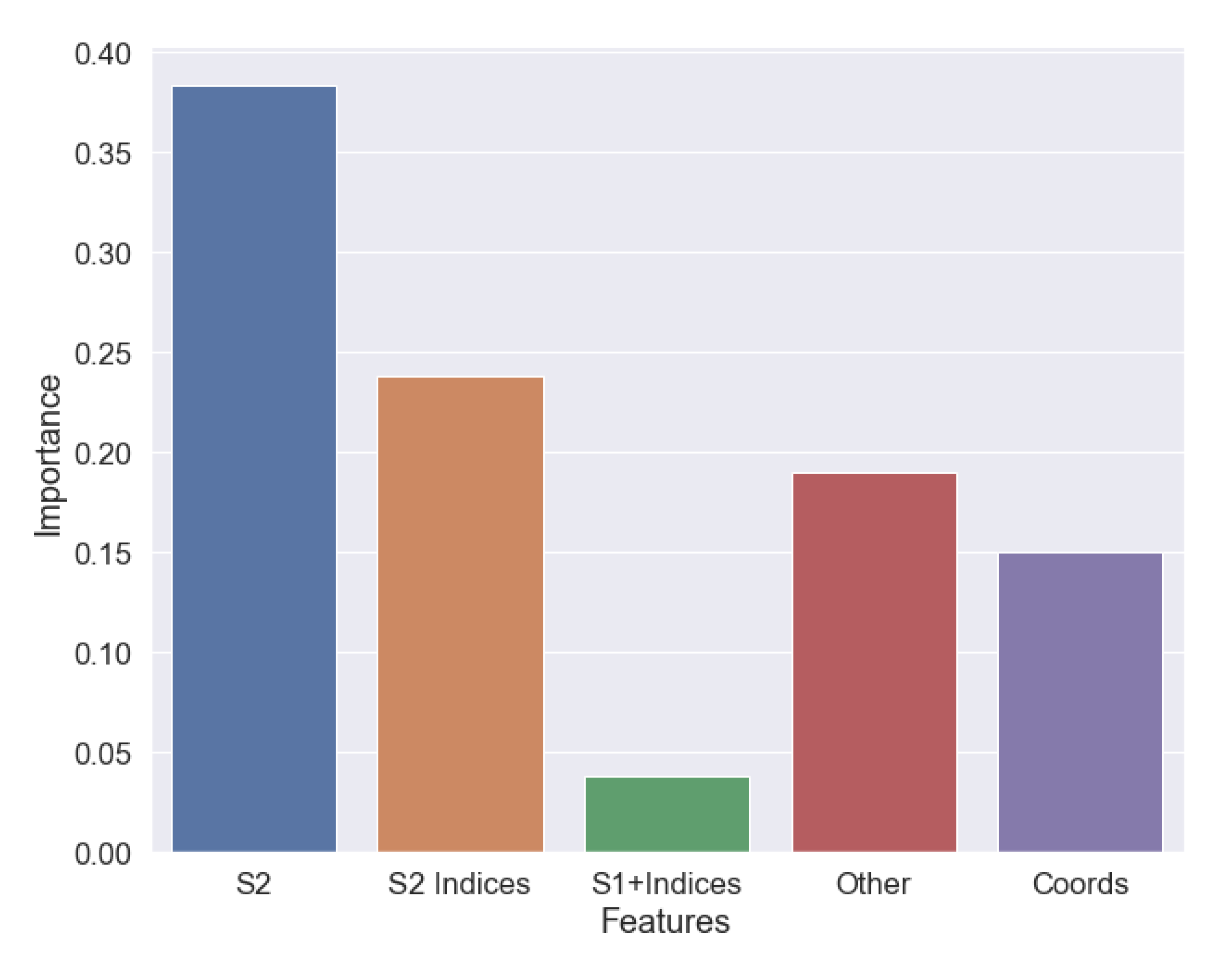
Figure 11 shows the importance of the characteristics in the final performance of the model, grouped by type. It can be seen that the S1 features were of little importance and that the S2 bands were the most important.
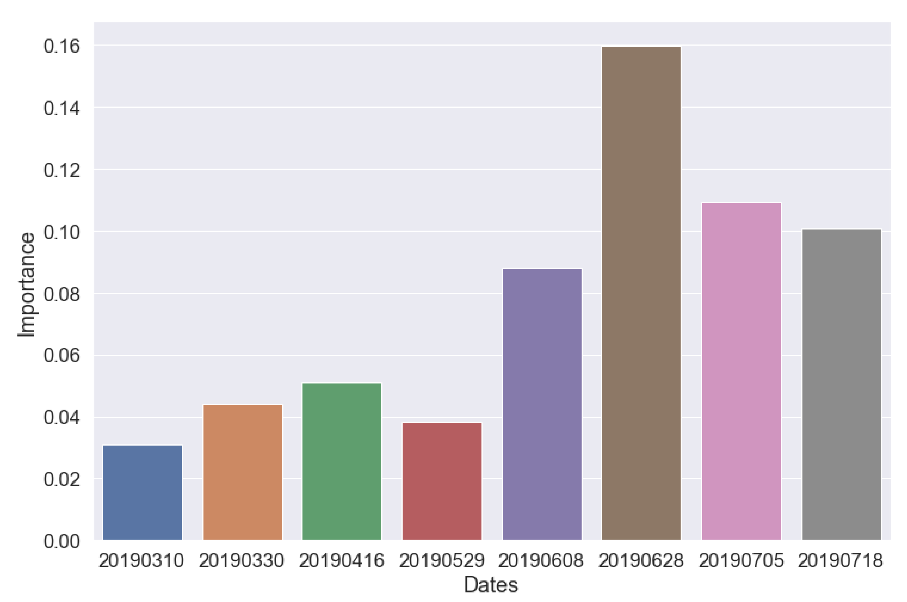
In
Figure 12, the relevance of each time series data in the generated model can be consulted. We can see how the initial dates had little impact on the final performance of the model.
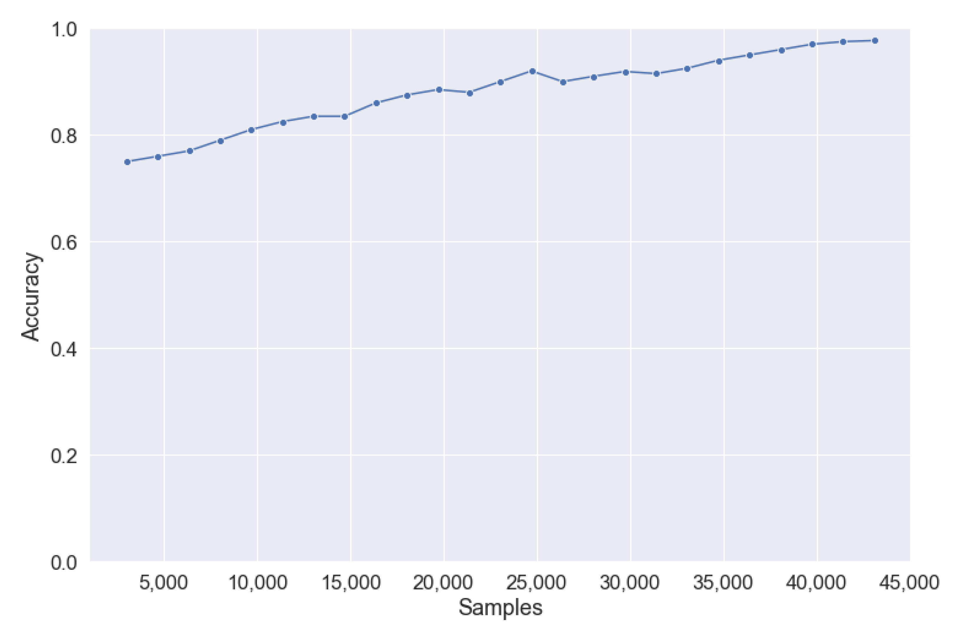
5.2.5. Learning Curve
Figure 13 shows the learning curve of the model generated in this work, in which the relationship between the number of samples and accuracy can be seen. It shows how a plateau was reached towards the end of the number of available samples.
6. Discussion
The objective of satellite image monitoring is to carry out a periodic and continuous control that verifies the status of an activity observed through a time series of images. This work has aimed to propose a methodology to automatically monitor the aid line for the protection of steppe birds promoted by the CAP, using Sentinel 1 and 2 missions and derived products that improve the decision-making process on granting aid. As part of the methodology, a traffic light map was developed to indicate which applications comply with the aid requirements (green) and which do not (red) [
24].
To achieve our objectives, we needed to use images from S1 and S2. Two methodologies with different approaches were proposed to choose the most suitable for the achievement of the proposed objective at the end of the process:
BirdsEO: proposes a strategy based on using more traditional remote sensing to combine different indices to see if the helpline conditions are met.
BirdsML: proposes combining ML algorithms with satellite imagery, mainly S1 and S2, and derived products (vegetation or polarised indices).
To achieve our goal, it was necessary to collect data for BirdsML from S2 without cloud cover; specifically, eight days were chosen. After selecting the images, different ML models were evaluated, RF was the one with the best metrics. Once the model was established, the model was optimized, finally obtaining values between 95–97% for all the monitored metrics. In the prediction phase, a pixel-level classification was obtained, then translated into a plot classification to get results like a traffic light. A threshold of 70% of predicted pixels was set with class 1 or Fulfill to establish which plot met the obligations. Furthermore, the BirdsEO methodology was inconclusive due to the crop typology, as the plant height did not allow results to be obtained using traditional remote sensing. The confusion created by satellite images to determine the plant’s height is due to the slope of the surface or the inclination of the plant caused by the wind. This problem is typical in radar images and S1 images too [
59,
60,
61] . Therefore the methodology finally proposed as a solution to the problem was BirdsML.
Different proposals in the literature address the issue of detecting crops such as cereals using ML models. Paper [
62] applies the use of time series on SAR S1 data, valid for the classification of several types of crops and determining that cereals have a different time signature than the rest of the crops. In paper [
63] they demonstrated that estimation of cover crop biomass is feasible using only VIs, as well as integrating optical remote sensing and SAR. Finally, paper [
64] presented a novel technique based on deep learning for crop type mapping, using NDVI time series for crop type mapping and compared with other advanced supervised learning techniques.
The BirdsML methodology can establish which applicants meet the conditions for this type of aid. These mechanisms represent progress in the digital transformation of public administrations, as it reduces the time spent on administrative tasks, improve efficiency in the management and granting of aid and generates savings in field trips or on-site controls. As weaknesses, we can highlight that the ground-truth dataset was unbalanced. For this reason, it would have been possible to develop further the application of techniques to balance it and check its repercussion on the model artificially. In addition, we could stop using traditional ML models and explore more carefully other more recent models such as LightGBM, XGBOOST, or even neural networks. The main idea is to improve the methodology during future campaigns by strengthening its weak points.
7. Conclusions
This work aimed to generate a methodology to discern whether applicants for aid for the protection of steppe birds complied with their commitments. These commitments include sowing medium or long-cycle cereal varieties and not harvesting before 15 July.
Two methodologies have been proposed to achieve the objective, one with a more traditional approach based on remote sensing (BirdsEO) and the other using Machine Learning (BirdsML). The first one used satellite images from the S1 and S2 missions to try to obtain an index as a solution. The second was based on combining data from different sources, such as time series of satellite images with their associated products, land uses and the aid applicant plots. This data was processed by applying Machine Learning techniques to judge whether an applicant was complying with the required obligations. In this way, we would end up with two results, and the final solution could be either of the two methodologies or a combination of both.
About the so-called BirdsEO methodology, certain impediments were encountered, mainly related to the land’s slope and the crop’s height. Therefore, the results were inconclusive, as they did not allow us to discern whether any medium or long-cycle cereal varieties were grown on the plots that applied for assistance.
In BirdsML, up to 14 different datasets were generated, and seven different Machine Learning classifiers were evaluated. The classifier that presented the most optimal results on the dataset with the highest number of features and the baseline definition was Random Forest, with 97% in metrics such as accuracy, recall and ROC-AUC Curve, and 95% in precision and recall. The LightGBM model also gave excellent results. As for the datasets generated, the one with the best metrics had the most significant number of features, called S2-S1-COOR-OTHER, which had a total of 156 independent variables, including a time series of satellite images S1 and S2, from 8 different dates.
At a more detailed level, it was found that the S1 data did not provide good metrics. On the other hand, contrary to what one might initially think, incorporating date-related features for each time series element into the Sentinel images did not help the model generalize better. Incorporating information related to the geographic location of the data offered a slight improvement in the model metrics.
Focusing on the importance of the features grouped by typology, it was observed that S2 data, grouping images and derived vegetation indices, summed about 70%, and S1 data (images + indices) only 4%. Characteristics related to land use and geographic location evenly distributed the remaining percentage.
Regarding the S2 time series dates, it was observed that the initial dates, when the crop is less developed, have little relevance to the model’s predictions.
Finally, we observed that a plateau phase was reached in the model learning curve towards the end of the maximum number of available samples, but it was not observed.
Among the improvements of this line of research is introducing the concept of feature engineering, whereby a compromise between dimensionality reduction of the ground-truth matrix and model performance would be sought, or whereby new relevant features such as agroclimatic information would be introduced [
65]. Another option could be working more deeply with the LightGBM model or neural networks.
Author Contributions
Conceptualization, F.J.L.-A., Z.H.-G., J.A.D.-G. and M.E.; methodology, F.J.L.-A., Z.H.-G., J.A.D.-G., J.A.L.-M. and M.E.; software, F.J.L.-A. and J.A.L.-M.; validation, Z.H.-G., J.A.D.-G., M.S.-A., J.A.C.-R. and M.E.; formal analysis, F.J.L.-A., Z.H.-G., J.A.D.-G. and M.E.; investigation, F.J.L.-A., Z.H.-G., J.A.D.-G. and M.E.; resources, Z.H.-G., J.F.A.-J., M.S.-A. and J.A.C.-R.; writing–original draft preparation, F.J.L.-A., J.F.A.-J., J.A.L.-M. and J.A.D.-G.; writing–review and editing, F.J.L.-A., J.A.L.-M., J.A.D.-G. and M.E.; visualization, J.F.A.-J., M.S.-A. and J.A.C.-R.; supervision, F.J.L.-A., Z.H.-G., J.A.L.-M. and M.E.; project administration, Z.H.-G. and M.S.-A.; funding acquisition, M.E. All authors have read and agreed to the published version of the manuscript.
Funding
This research was funded by the European Regional Development Fund (ERDF), through project FEDER 14-20-25 “Impulso a la economía circular en la agricultura y la gestión del agua mediante el uso avanzado de nuevas tecnologías-iagua”.
Data Availability Statement
Data sharing not applicable.
Acknowledgments
The authors thank the European Space Agency, the European Commission, and the Copernicus Programme.
Conflicts of Interest
The authors declare no conflict of interest.
Appendix A
The workflow followed during this project is shown in
Table A1.
Table A1.
Activity schedule.
Table A1.
Activity schedule.
| Activity | Methodology | Activity Period |
|---|
| State of Art | BirdsEO, BirdsML | July-2019 & September-2019 |
| Radiometry Campaigns | BirdsEO | July-2019 & September-2019 |
| UAV Campaigns | BirdsEO | July-2019 & September-2019 |
| Survey123 Campaigns | BirdsEO, BirdsML | July-2019 & September-2019 |
| S1&S2 Download | BirdsEO, BirdsML | July-2019 & September-2019 |
| S1&S2 Indices Generation | BirdsEO, BirdsML | July-2019 & September-2019 |
| S1&S2 Indices Analysis | BirdsEO, BirdsML | July-2019 & September-2019 |
| Machine Learning | BirdsML | January-2020 & December-2021 |
| Paper and Report | BirdsEO, BirdsML | January-2022 & June-2022 |
References
- PanEuropean Common Bird Monitoring Scheme. Available online: https://pecbms.info/ (accessed on 12 November 2021).
- Traba, J.; Morales, M.B. The decline of farmland birds in Spain is strongly associated to the loss of fallowland. Sci. Rep. 2019, 9, 9473. [Google Scholar] [CrossRef]
- Matthews, A. The European Union’s common agricultural policy and developing countries: The struggle for coherence. Eur. Integr. 2008, 30, 381–399. [Google Scholar] [CrossRef]
- Tarjuelo, R.; Margalida, A.; Mougeot, F. Changing the fallow paradigm: A win–win strategy for the post-2020 Common Agricultural Policy to halt farmland bird declines. J. Appl. Ecol. 2020, 57, 642–649. [Google Scholar] [CrossRef]
- Regulation 1307/2013. Available online: https://eur-lex.europa.eu/legal-content/EN/TXT/PDF/?uri=CELEX:32013R1307 (accessed on 28 October 2021).
- Regulation 1306/2013. Available online: https://eur-lex.europa.eu/legal-content/EN/TXT/PDF/?uri=CELEX:32013R1306&from=en (accessed on 21 October 2021).
- Regulation 2018/746. Available online: https://eur-lex.europa.eu/legal-content/EN/TXT/PDF/?uri=CELEX:32018R0746&from=EN (accessed on 2 April 2021).
- Wójtowicz, M.; Wójtowicz, A.; Piekarczyk, J. Application of remote sensing methods in agriculture. Commun. Biometry Crop. Sci. 2016, 11, 31–50. [Google Scholar]
- Shanmugapriya, P.; Rathika, S.; Ramesh, T.; Janaki, P. Applications of remote sensing in agriculture—A Review. Int. J. Curr. Microbiol. Appl. Sci. 2019, 8, 2270–2283. [Google Scholar] [CrossRef]
- Bousbih, S.; Zribi, M.; Lili-Chabaane, Z.; Baghdadi, N.; El Hajj, M.; Gao, Q.; Mougenot, B. Potential of Sentinel-1 radar data for the assessment of soil and cereal cover parameters. Sensors 2017, 17, 2617. [Google Scholar] [CrossRef] [Green Version]
- Van Tricht, K.; Gobin, A.; Gilliams, S.; Piccard, I. Synergistic use of radar Sentinel-1 and optical Sentinel-2 imagery for crop mapping: A case study for Belgium. Remote Sens. 2018, 10, 1642. [Google Scholar] [CrossRef] [Green Version]
- Rouse, J.; Haas, R.; Schell, J.; Deering, D. Monitoring vegetation systems in the great plains with ERTS proceeding. In Third Earth Reserves Technology Satellite Symposium; NASA: Greenbelt, MD, USA, 1974; SP-351; Volume 30103017. [Google Scholar]
- Tucker, C.J. Red and photographic infrared linear combinations for monitoring vegetation. Remote Sens. Environ. 1979, 8, 127–150. [Google Scholar] [CrossRef] [Green Version]
- Copernicus Global Land Service. Available online: https://land.copernicus.eu/global/products/ndvi (accessed on 4 May 2021).
- Sultana, S.R.; Ali, A.; Ahmad, A.; Mubeen, M.; Zia-Ul-Haq, M.; Ahmad, S.; Ercisli, S.; Jaafar, H.Z. Normalized difference vegetation index as a tool for wheat yield estimation: A case study from Faisalabad, Pakistan. Sci. World J. 2014, 2014, 725326. [Google Scholar] [CrossRef] [Green Version]
- Chao Rodríguez, Y.; El Anjoumi, A.; Domínguez Gómez, J.; Rodríguez Pérez, D.; Rico, E. Using Landsat image time series to study a small water body in Northern Spain. Environ. Monit. Assess. 2014, 186, 3511–3522. [Google Scholar] [CrossRef]
- Domínguez, J.A.; Kumhálová, J.; Novák, P. Winter oilseed rape and winter wheat growth prediction using remote sensing methods. Plant Soil Environ. 2015, 61, 410–416. [Google Scholar]
- Echavarría-Caballero, C.; Domínguez-Gómez, J.A.; González-García, C.; García-García, M.J. Water quality spatial-temporal analysis of gravel pit ponds in the southeast regional park Madrid (Spain) from 1984 to 2009. Geocarto Int. 2022. Available online: https://0-www-tandfonline-com.brum.beds.ac.uk/doi/epub/10.1080/10106049.2022.2037736?needAccess=true (accessed on 6 April 2022). [CrossRef]
- Wardlow, B.D.; Egbert, S.L.; Kastens, J.H. Analysis of time-series MODIS 250 m vegetation index data for crop classification in the US Central Great Plains. Remote Sens. Environ. 2007, 108, 290–310. [Google Scholar] [CrossRef] [Green Version]
- Shrestha, A.B. Enhancing Temporal Series of Sentinel-2 and Sentinel-3 Data Products: From Classical Regression to Deep Learning Approach. Ph.D. Thesis, Universidade NOVA de Lisboa, Lisbon, Portugal, 2021. [Google Scholar]
- Wagner, W.; Bauer-Marschallinger, B.; Navacchi, C.; Reuß, F.; Cao, S.; Reimer, C.; Schramm, M.; Briese, C. A Sentinel-1 backscatter datacube for global land monitoring applications. Remote Sens. 2021, 13, 4622. [Google Scholar] [CrossRef]
- Open Data Cube. Available online: https://www.opendatacube.org/overview (accessed on 21 May 2021).
- Data Application of the Month: Earth Observation Data Cubes. Available online: https://www.un-spider.org/links-and-resources/daotm-data-cubes (accessed on 15 January 2022).
- López-Andreu, F.J.; Erena, M.; Dominguez-Gómez, J.A.; López-Morales, J.A. Sentinel-2 images and machine learning as tool for monitoring of the common agricultural policy: Calasparra rice as a case study. Agronomy 2021, 11, 621. [Google Scholar] [CrossRef]
- López-Andreu, F.J.; López-Morales, J.A.; Erena, M.; Skarmeta, A.F.; Martínez, J.A. Monitoring System for the Management of the Common Agricultural Policy Using Machine Learning and Remote Sensing. Electronics 2022, 11, 325. [Google Scholar] [CrossRef]
- Tenreiro, T.R.; García-Vila, M.; Gómez, J.A.; Jiménez-Berni, J.A.; Fereres, E. Using NDVI for the assessment of canopy cover in agricultural crops within modelling research. Comput. Electron. Agric. 2021, 182, 106038. [Google Scholar] [CrossRef]
- García, M.J.V. Atlas Global de la Región de Murcia/Coordinación Científica, Asunción Romero Díaz; Coordinación Cartográfica, Francisco Alonso Sarría: Reseña Bibliográfica; Universidad de Murcia: Murcia, Spain, 2008; Volume 24, Available online: https://digitum.um.es/digitum/handle/10201/11948 (accessed on 5 May 2022).
- European Space Agency. Available online: https://www.esa.int (accessed on 5 May 2022).
- Filipponi, F. Sentinel-1 GRD preprocessing workflow. Multidiscip. Digit. Publ. Inst. Proc. 2019, 18, 11. [Google Scholar]
- Daughtry, C.S.; Walthall, C.; Kim, M.; De Colstoun, E.B.; McMurtrey Iii, J. Estimating corn leaf chlorophyll concentration from leaf and canopy reflectance. Remote Sens. Environ. 2000, 74, 229–239. [Google Scholar] [CrossRef]
- Rondeaux, G.; Steven, M.; Baret, F. Optimization of soil-adjusted vegetation indices. Remote Sens. Environ. 1996, 55, 95–107. [Google Scholar] [CrossRef]
- Lee, J.S. Speckle analysis and smoothing of synthetic aperture radar images. Comput. Graph. Image Process. 1981, 17, 24–32. [Google Scholar] [CrossRef]
- Lee, J.S.; Grunes, M.R.; De Grandi, G. Polarimetric SAR speckle filtering and its implication for classification. IEEE Trans. Geosci. Remote Sens. 1999, 37, 2363–2373. [Google Scholar]
- Lee, J.S.; Wen, J.H.; Ainsworth, T.L.; Chen, K.S.; Chen, A.J. Improved sigma filter for speckle filtering of SAR imagery. IEEE Trans. Geosci. Remote Sens. 2008, 47, 202–213. [Google Scholar]
- e Santos, D.A.; Martinez, J.; Harmel, T.; Borges, H.; Roig, H. Evaluation of Sentinel-2/Msi Imagery Products Level-2a Obtained by Three Different Atmospheric Corrections for Monitoring Suspended Sediments Concentration in Madeira River, Brazil. In Proceedings of the IEEE Latin American GRSS & ISPRS Remote Sensing Conference (LAGIRS), Santiago, Chile, 22–26 March 2020; pp. 207–212. [Google Scholar]
- Gitelson, A.A.; Kaufman, Y.J.; Merzlyak, M.N. Use of a green channel in remote sensing of global vegetation from EOS-MODIS. Remote Sens. Environ. 1996, 58, 289–298. [Google Scholar] [CrossRef]
- Huete, A.R. A soil-adjusted vegetation index (SAVI). Remote Sens. Environ. 1988, 25, 295–309. [Google Scholar] [CrossRef]
- SIGPAC. Available online: https://sigpac.mapa.gob.es/fega/visor/ (accessed on 6 May 2022).
- CNIG. Available online: https://centrodedescargas.cnig.es/CentroDescargas/index.jsp (accessed on 6 May 2022).
- Li, Y.; Chen, J.; Ma, Q.; Zhang, H.K.; Liu, J. Evaluation of Sentinel-2A surface reflectance derived using Sen2Cor in North America. IEEE J. Sel. Top. Appl. Earth Obs. Remote Sens. 2018, 11, 1997–2021. [Google Scholar] [CrossRef]
- Tsouros, D.C.; Bibi, S.; Sarigiannidis, P.G. A review on UAV-based applications for precision agriculture. Information 2019, 10, 349. [Google Scholar] [CrossRef] [Green Version]
- Hunt, E.R.; Cavigelli, M.; Daughtry, C.S.; Mcmurtrey, J.E.; Walthall, C.L. Evaluation of digital photography from model aircraft for remote sensing of crop biomass and nitrogen status. Precis. Agric. 2005, 6, 359–378. [Google Scholar] [CrossRef]
- Gobron, N.; Pinty, B.; Verstraete, M.M.; Widlowski, J.L. Advanced vegetation indices optimized for up-coming sensors: Design, performance, and applications. IEEE Trans. Geosci. Remote Sens. 2000, 38, 2489–2505. [Google Scholar]
- Hunt, E.R., Jr.; Doraiswamy, P.C.; McMurtrey, J.E.; Daughtry, C.S.; Perry, E.M.; Akhmedov, B. A visible band index for remote sensing leaf chlorophyll content at the canopy scale. Int. J. Appl. Earth Obs. Geoinf. 2013, 21, 103–112. [Google Scholar] [CrossRef] [Green Version]
- Bendig, J.; Yu, K.; Aasen, H.; Bolten, A.; Bennertz, S.; Broscheit, J.; Gnyp, M.L.; Bareth, G. Combining UAV-based plant height from crop surface models, visible, and near infrared vegetation indices for biomass monitoring in barley. Int. J. Appl. Earth Obs. Geoinf. 2015, 39, 79–87. [Google Scholar] [CrossRef]
- Gitelson, A.A.; Kaufman, Y.J.; Stark, R.; Rundquist, D. Novel algorithms for remote estimation of vegetation fraction. Remote Sens. Environ. 2002, 80, 76–87. [Google Scholar] [CrossRef] [Green Version]
- SNAP. Available online: https://step.esa.int/main/download/snap-download/ (accessed on 15 October 2021).
- Kobayashi, N.; Tani, H.; Wang, X.; Sonobe, R. Crop classification using spectral indices derived from Sentinel-2A imagery. J. Inf. Telecommun. 2020, 4, 67–90. [Google Scholar] [CrossRef]
- Zarco-Tejada, P.J.; Miller, J.R.; Noland, T.L.; Mohammed, G.H.; Sampson, P.H. Scaling-up and model inversion methods with narrowband optical indices for chlorophyll content estimation in closed forest canopies with hyperspectral data. IEEE Trans. Geosci. Remote Sens. 2001, 39, 1491–1507. [Google Scholar] [CrossRef] [Green Version]
- Gitelson, A.A.; Chivkunova, O.B.; Merzlyak, M.N. Nondestructive estimation of anthocyanins and chlorophylls in anthocyanic leaves. Am. J. Bot. 2009, 96, 1861–1868. [Google Scholar] [CrossRef]
- Gitelson, A.A.; Merzlyak, M.N.; Chivkunova, O.B. Optical properties and nondestructive estimation of anthocyanin content in plant leaves. Photochem. Photobiol. 2001, 74, 38–45. [Google Scholar] [CrossRef]
- Wu, C.; Niu, Z.; Tang, Q.; Huang, W. Estimating chlorophyll content from hyperspectral vegetation indices: Modeling and validation. Agric. For. Meteorol. 2008, 148, 1230–1241. [Google Scholar] [CrossRef]
- Ramezan, C.A.; Warner, T.A.; Maxwell, A.E. Evaluation of sampling and cross-validation tuning strategies for regional-scale machine learning classification. Remote Sens. 2019, 11, 185. [Google Scholar] [CrossRef] [Green Version]
- Kaur, H.; Pannu, H.S.; Malhi, A.K. A systematic review on imbalanced data challenges in machine learning: Applications and solutions. ACM Comput. Surv. (CSUR) 2019, 52, 1–36. [Google Scholar] [CrossRef] [Green Version]
- Chen, T.; He, T.; Benesty, M.; Khotilovich, V.; Tang, Y.; Cho, H.; Chen, K. Xgboost: Extreme Gradient Boosting; R Package Version 0.4-2; 2015; Volume 1, pp. 1–4. Available online: https://cran.microsoft.com/snapshot/2017-12-11/web/packages/xgboost/vignettes/xgboost.pdf (accessed on 19 September 2021).
- Ke, G.; Meng, Q.; Finley, T.; Wang, T.; Chen, W.; Ma, W.; Ye, Q.; Liu, T.Y. Lightgbm: A highly efficient gradient boosting decision tree. Adv. Neural Inf. Process. Syst. 2017, 30, 3147–3155. [Google Scholar]
- Carvalho, D.V.; Pereira, E.M.; Cardoso, J.S. Machine learning interpretability: A survey on methods and metrics. Electronics 2019, 8, 832. [Google Scholar] [CrossRef] [Green Version]
- ArcGIS Survey123. Available online: https://survey123.arcgis.com/ (accessed on 19 September 2021).
- Abdikan, S.; Sekertekin, A.; Ustunern, M.; Sanli, F.B.; Nasirzadehdizaji, R. Backscatter analysis using multi-temporal Sentinel-1 SAR data for crop growth of maize in Konya Basin, Turkey. Int. Arch. Photogramm. Remote Sens. Spat. Inf. Sci 2018, 42, 9–13. [Google Scholar] [CrossRef] [Green Version]
- Dirgahayu, D.; Parsa, I.M. Detection Phase Growth of Paddy Crop Using SAR Sentinel-1 Data. In Proceedings of the IOP Conference Series: Earth and Environmental Science, Moscow, Russia, 27 May–6 June 2019; Volume 280, p. 012020. [Google Scholar]
- Schiavon, E.; Taramelli, A.; Tornato, A.; Pierangeli, F. Monitoring environmental and climate goals for European agriculture: User perspectives on the optimization of the Copernicus evolution offer. J. Environ. Manag. 2021, 296, 113121. [Google Scholar] [CrossRef]
- Arias, M.; Campo-Bescós, M.Á.; Álvarez-Mozos, J. Crop classification based on temporal signatures of Sentinel-1 observations over Navarre province, Spain. Remote Sens. 2020, 12, 278. [Google Scholar] [CrossRef] [Green Version]
- Jennewein, J.S.; Lamb, B.T.; Hively, W.D.; Thieme, A.; Thapa, R.; Goldsmith, A.; Mirsky, S.B. Integration of Satellite-Based Optical and Synthetic Aperture Radar Imagery to Estimate Winter Cover Crop Performance in Cereal Grasses. Remote Sens. 2022, 14, 2077. [Google Scholar] [CrossRef]
- Seydi, S.T.; Amani, M.; Ghorbanian, A. A Dual Attention Convolutional Neural Network for Crop Classification Using Time-Series Sentinel-2 Imagery. Remote Sens. 2022, 14, 498. [Google Scholar] [CrossRef]
- Erena, M.; López, J.; García, P.; Caro, M.; Belda, F.; Palenzuela, J.; Toledano, F.; Torralba, P.; González-Barbera, G.; García-Pintado, J. Estimación de precipitación combinada radar-pluviómetros y publicación mediante servicios OGC. XV CNTIG. CSIC 2012, 1, 412–419. [Google Scholar]
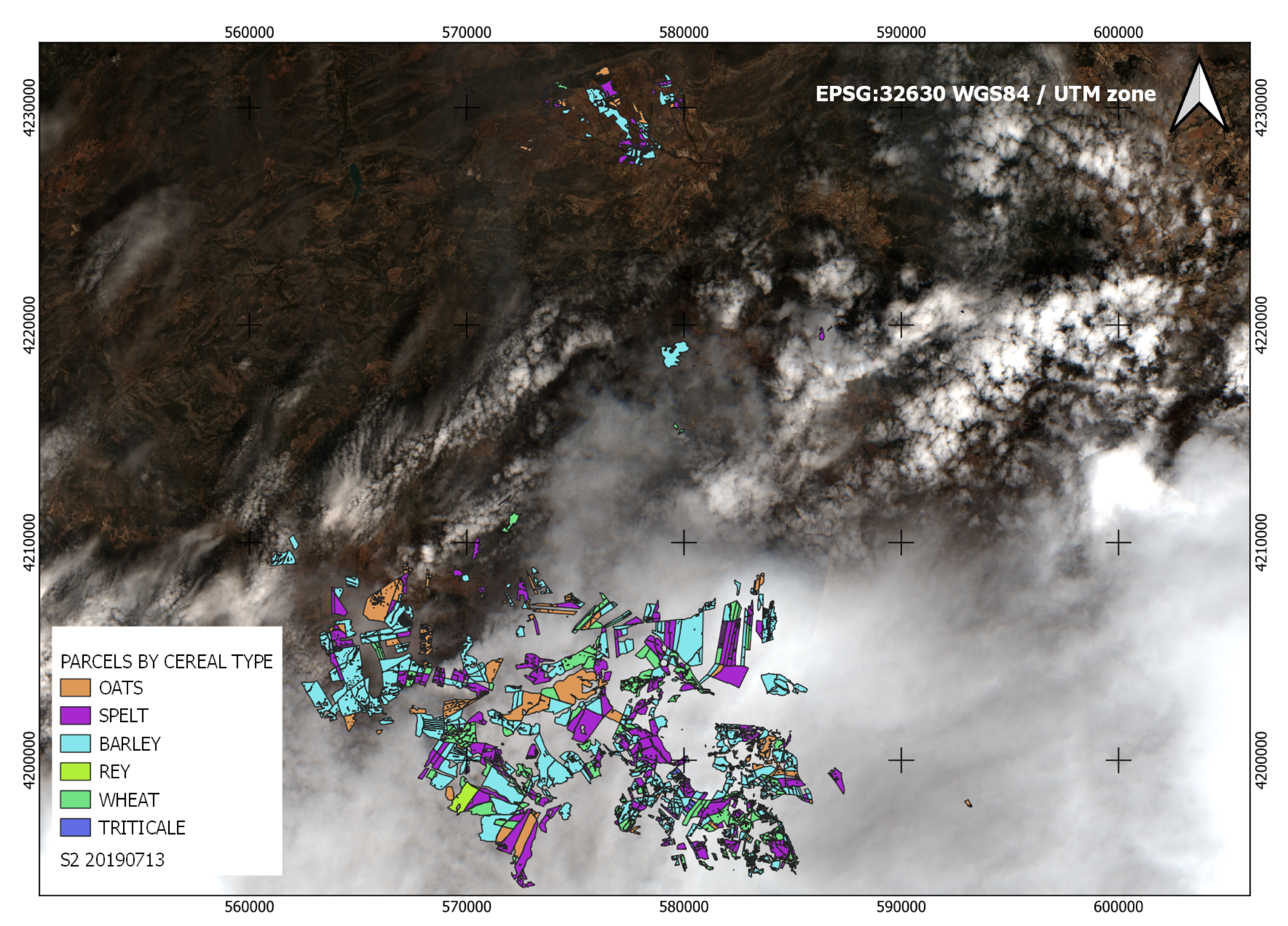
Figure 1.
Study area in the Autonomous Community of the Region of Murcia.
Figure 1.
Study area in the Autonomous Community of the Region of Murcia.
Figure 2.
Planning according to decision tree.
Figure 2.
Planning according to decision tree.
Figure 3.
Field data campaigns. (a) Radiometry. (b) UAV.
Figure 3.
Field data campaigns. (a) Radiometry. (b) UAV.
Figure 4.
BirdsML methodology scheme.
Figure 4.
BirdsML methodology scheme.
Figure 5.
BirdsML methodology scheme.
Figure 5.
BirdsML methodology scheme.
Figure 6.
From pixel-level to object-level classification. (a) BirdsML prediction. (b) Results as traffic light system.
Figure 6.
From pixel-level to object-level classification. (a) BirdsML prediction. (b) Results as traffic light system.
Figure 7.
Example of the ITSSC file (in red the pilot areas).
Figure 7.
Example of the ITSSC file (in red the pilot areas).
Figure 8.
Example of the cloud cover with the pilot areas on 13 July 2019, the first image after the deadline (15 July).
Figure 8.
Example of the cloud cover with the pilot areas on 13 July 2019, the first image after the deadline (15 July).
Figure 9.
Map of (NDPVH-VV) as a function of the change threshold.
Figure 9.
Map of (NDPVH-VV) as a function of the change threshold.
Figure 10.
Time series of various covers. (a,b) Harvested Cereal. (c,d) Unharvested Cereal.
Figure 10.
Time series of various covers. (a,b) Harvested Cereal. (c,d) Unharvested Cereal.
Figure 11.
Importance of characteristics grouped by typology.
Figure 11.
Importance of characteristics grouped by typology.
Figure 12.
Relevance of time series dates.
Figure 12.
Relevance of time series dates.
Figure 13.
Learning curve of the model.
Figure 13.
Learning curve of the model.
Table 1.
Characteristics of S2 bands used.
Table 1.
Characteristics of S2 bands used.
| Band | Resolution (m) | Wavelength (nm) | Description |
|---|
| B1 | 60 | 0.443 | Aerosol |
| B2 | 10 | 0.490 | Blue |
| B3 | 10 | 0.560 | Green |
| B4 | 10 | 0.665 | Red |
| B5 | 20 | 0.705 | Red edge 1 |
| B6 | 20 | 0.740 | Red edge 2 |
| B7 | 20 | 0.783 | Red edge 3 |
| B8 | 10 | 0.842 | Near infrared |
| B9 | 60 | 0.945 | Water vapor |
| B10 | 60 | 1.375 | Cirrus |
| B11 | 20 | 1.610 | SWIR 1 |
| B12 | 20 | 2.190 | SWIR 2 |
Table 2.
Distribution among classes of the ground-truth data.
Table 2.
Distribution among classes of the ground-truth data.
| Class | Pixels | Percentage |
|---|
| Fulfill (1) | 34,304 | 80 |
| Not Fulfill (99) | 8792 | 20 |
Table 3.
Features of the generated datasets.
Table 3.
Features of the generated datasets.
| Dataset | S2 + Indices | S1 + Indices | Date | Coords. | SIGPAC | DEM | Features |
|---|
| S2 | ✓ | | | | | | 120 |
| S2-COOR | ✓ | | | ✓ | | | 122 |
| S2-DATE | ✓ | | ✓ | | | | 125 |
| S2-OTHER | ✓ | | | | ✓ | ✓ | 122 |
| S2-COOR-OTHER | ✓ | | | ✓ | ✓ | ✓ | 124 |
| S1 | | ✓ | | | | | 32 |
| S1-COOR | | ✓ | | ✓ | | | 34 |
| S1-DATE | | ✓ | ✓ | | | | 37 |
| S1-OTHER | | | | | | | 34 |
| S1-COOR-OTHER | | ✓ | | ✓ | ✓ | ✓ | 36 |
| S2-S1 | ✓ | ✓ | | | | | 152 |
| S2-S1-COOR | ✓ | ✓ | | ✓ | | | 154 |
| S2-S1-OTHER | ✓ | ✓ | | | ✓ | ✓ | 154 |
| S2-S1-COOR-OTHER | ✓ | ✓ | | ✓ | ✓ | ✓ | 156 |
Table 4.
Metrics obtained during the model selection phase.
Table 4.
Metrics obtained during the model selection phase.
| Model | Metrics (%) |
|---|
| ACC | Kappa | Precision | Recall | F1 | AUC-ROC Curve |
|---|
| KNN | 96.75 ± 10.39 | 93.37 ± 19.26 | 93.31 ± 17.43 | 93.89 ± 4.36 | 95.23 ± 13.54 | 95.55 ± 8.19 |
| CART | 93.44 ± 15.12 | 85.58 ± 25.66 | 88.97 ± 20.66 | 93.95 ± 16.75 | 88.99 ± 19.15 | 93.63 ± 12.43 |
| EXT | 96.36 ± 11.31 | 91.58 ± 22.42 | 94.47 ± 17.61 | 93.99 ± 12.85 | 93.70 ± 16.04 | 95.48 ± 11.48 |
| BG | 92.75 ± 15.13 | 83.87 ± 25.95 | 87.12 ± 21.51 | 93.60 ± 16.85 | 87.70 ± 19.36 | 93.08 ± 12.45 |
| RF | 97.40 ± 5.52 | 93.14 ± 11.10 | 94.98 ± 9.27 | 95.31 ± 6.51 | 94.75 ± 6.49 | 96.62 ± 5.70 |
| XGB | 96.63 ± 7.33 | 90.72 ± 19.47 | 93.67 ± 16.13 | 94.93 ± 15.55 | 92.63 ± 15.69 | 96.00 ± 8.98 |
| LGBM | 96.75 ± 5.45 | 92.64 ± 14.81 | 93.71 ± 13.65 | 95.06 ± 10.11 | 94.06 ± 11.35 | 96.12 ± 6.92 |
Table 5.
Metrics obtained by Random Forest for each of the generated datasets.
Table 5.
Metrics obtained by Random Forest for each of the generated datasets.
| Dataset | Metrics (%) |
|---|
| ACC | Kappa | Precision | Recall | F1 | ROC-AUC Curve |
|---|
| S2 | 95.28 ± 8.97 | 86.34 ± 24.49 | 90.02 ± 20.33 | 89.63 ± 19.13 | 89.32 ± 18.78 | 93.18 ± 12.47 |
| S2-COOR | 96.92 ± 8.13 | 91.49 ± 22.33 | 93.67 ± 19.17 | 93.91 ± 15.76 | 93.44 ± 17.17 | 95.80 ± 10.69 |
| S2-DATE | 94.06 ± 8.99 | 81.26 ± 26.05 | 91.32 ± 20.32 | 81.58 ± 23.03 | 84.80 ± 20.66 | 89.42 ± 13.75 |
| S2-OTHER | 95.12 ± 11.19 | 89.40 ± 21.05 | 90.83 ± 20.14 | 96.59 ± 6.03 | 92.24 ± 14.85 | 95.66 ± 8.42 |
| S2-COOR-OTHER | 97.84 ± 6.14 | 94.46 ± 14.44 | 95.04 ± 13.74 | 97.33 ± 6.43 | 95.81 ± 10.64 | 97.65 ± 6.05 |
| S1 | 82.61 ± 8.46 | 26.73 ± 34.52 | 63.34 ± 35.36 | 26.11 ± 30.88 | 32.46 ± 32.44 | 61.59 ± 16.37 |
| S1-COOR | 92.85 ± 9.89 | 80.67 ± 24.82 | 88.14 ± 21.44 | 89.36 ± 22.30 | 84.62 ± 20.08 | 91.5 ± 11.69 |
| S1-DATE | 90.53 ± 9.97 | 16.73 ± 35.21 | 64.52 ± 36.11 | 18.38 ± 33.69 | 27.12 ± 37.28 | 57.64 ± 18.73 |
| S1-OTHER | 91.82 ± 12.59 | 82.40 ± 24.52 | 83.05 ± 24.56 | 97.03 ± 5.39 | 87.19 ± 17.41 | 93.76 ± 8.43 |
| S1-COOR-OTHER | 96.19 ± 7.48 | 89.87 ± 19.30 | 92.18 ± 17.18 | 96.05 ± 15.07 | 92.05 ± 15.47 | 96.13 ± 8.45 |
| S2-S1 | 94.92 ± 9.33 | 84.81 ± 24.04 | 92.43 ± 19.48 | 85.38 ± 17.23 | 87.87 ± 18.24 | 91.37 ± 11.77 |
| S2-S1-COOR | 96.43 ± 8.25 | 90.38 ± 21.21 | 93.70 ± 18.71 | 92.88 ± 14.59 | 92.60 ± 16.05 | 95.11 ± 9.96 |
| S2-S1-OTHER | 95.10 ± 11.27 | 89.44 ± 21.17 | 94.79 ± 20.17 | 97.33 ± 5.75 | 95.67 ± 14.92 | 97.61 ± 8.44 |
| S2-S1-COOR-OTHER | 97.77 ± 3.09 | 94.29 ± 7.26 | 94.79 ± 6.90 | 97.33 ± 3.25 | 95.67 ± 5.35 | 97.61 ± 3.04 |
| Publisher’s Note: MDPI stays neutral with regard to jurisdictional claims in published maps and institutional affiliations. |
© 2022 by the authors. Licensee MDPI, Basel, Switzerland. This article is an open access article distributed under the terms and conditions of the Creative Commons Attribution (CC BY) license (https://creativecommons.org/licenses/by/4.0/).

 ,
, 


