
Development of a Crop Spectral Reflectance Sensor
by
 , ,
, ,
Naisen Liu
1,2,3,*,† ,
,
Wenyu Zhang
4,5,6,7,†,
Fuxia Liu
1,2,3,
Meina Zhang
4,5,6,7,
Chenggong Du
1,2,3,
Chuanliang Sun
4,5,6,
Jing Cao
4,5,6,
Shuwen Ji
1,2,3 and
Hui Sun
1,2,3 1
Jiangsu Collaborative Innovation Center of Regional Modern Agriculture & Environmental Protection, Huaiyin Normal University, Huai’an 223300, China
2
Jiangsu Key Laboratory for Eco-Agricultural Biotechnology around Hongze Lake, Huaiyin Normal University, Huai’an 223300, China
3
Jiangsu Engineering Research Center for Cyanophytes Forecast and Ecological Restoration of Hongze Lake, Huaiyin Normal University, Huai’an 223300, China
4
IGRB-IAI Joint Laboratory of Germplasm Resources Innovation & Information Utilization, Jiangsu Academy of Agricultural Sciences, Nanjing 210014, China
5
YuanQi-IAI Joint Laboratory for Agricultural Digital Twin, Jiangsu Academy of Agricultural Sciences, Nanjing 210014, China
6
Institute of Agricultural Information, Jiangsu Academy of Agricultural Sciences, Nanjing 210014, China
7
School of Agricultural Engineering, Jiangsu University, Zhenjiang 212013, China
*
Author to whom correspondence should be addressed.
†
These authors contributed equally to this work.
Agronomy 2022, 12(9), 2139; https://0-doi-org.brum.beds.ac.uk/10.3390/agronomy12092139
Submission received: 23 July 2022
/
Revised: 5 September 2022
/
Accepted: 5 September 2022
/
Published: 8 September 2022
(This article belongs to the Special Issue Frontier Studies in Crop Growth Monitoring, Diagnosis and Precision Operation)
Abstract
:In this study, a low-cost, self-balancing crop spectral reflectance sensor (CSRS) was designed for real-time, nondestructive monitoring of the spectral reflectance and vegetation index of crops such as tomato and rapeseed. The sensor had a field of view of 30°, and a narrow-band filter was used for light splitting. The filter’s full width at half-maximum was 10 nm, and the spectral bands were 710 nm and 870 nm. The sensor was powered by a battery and used WiFi for communication. Its software was based on the Contiki operating system. To make the sensor work in different light intensity conditions, the photoelectric conversion automatic gain circuit had a total of 255 combinations of amplification. The gimbal of the sensor was mainly composed of an inner ring and an outer ring. Under the gravity of the sensor, the central axis of the sensor remained vertical, such that the up-facing and down-facing photosensitive units stayed in the horizontal position. The mechanical components of the sensor were designed symmetrically to facilitate equal mass distribution and to meet the needs of automatic balancing. Based on the optical signal transmission process of the sensor and the dark-current characteristics of the photodetector, a calibration method was theoretically deduced, which improved the accuracy and stability of the sensor under different ambient light intensities. The calibration method is also applicable for the calibration of other crop growth information sensors. Next, the standard reflectance gray scale was taken as the measurement variable to test the accuracy of the sensor, and the results showed that the root mean square error of the reflectance measured by the sensor at 710 nm and 870 nm was 1.10% and 1.27%, respectively; the mean absolute error was 0.95% and 0.89%, respectively; the relative error was below 4% and 3%, respectively; and the coefficient of variation was between 1.0% and 2.5%. The reflectance data measured by the sensor under different ambient light intensities suggested that the absolute error of the sensor was within ±0.5%, and the coefficients of variation at the two spectral bands were 1.04% and 0.39%, respectively. With tomato and rapeseed as the monitoring targets, the proposed CSRS and a commercial spectroradiometer were used to measure at the same time. The results showed that the reflectance measured by the two devices was very close, and there was a linear relationship between the normalized difference vegetation index of the CSRS and that of the commercial spectroradiometer. The coefficient of determination (R2) for tomato and rapeseed were 0.9540 and 0.9110, respectively.
1. Introduction
Crop growth information is of great importance for crop growth regulation in agricultural production, and the result of regulation directly affects the yield or quality of crops [1,2,3,4]. Therefore, crop growth information is essential for precision agriculture/smart farming. Since the 20th century, remote sensing has been used to monitor and obtain agricultural information [5], such as yield or biomass [6,7,8,9,10], chlorophyll content [11], leaf nitrogen content [12], and leaf area index [13,14,15]. By measuring the reflectance spectrum of a crop canopy, we can obtain biological growth information nondestructively in real time, and this method has the advantages of high resolution and accuracy [16]. Zhu et al. reported that 810 nm and 870 nm were two single common spectral wavebands indicating leaf nitrogen accumulation (LNA) in wheat, and the ratio vegetation index (RVI) at 810 nm and 660 nm had higher accuracy [17]. Based on the spectral reflectance at 423, 703, and 924 nm, Wang et al. constructed a three-band vegetation index to estimate the leaf nitrogen concentration (LNC) of rice and wheat. The coefficient of determination (R2) of the model was greater than 0.85 [18]. Cao et al. constructed the normalized difference spectral index (NDSI) based on spectral information at 730 nm and 940 nm and the modified normalized difference spectral index (mNDSI) based on spectral information at 730, 940, and 950 nm. Then, NDSI and mNDSI were used to predict the leaf area index (LAI), and the influence of spectral saturation on the prediction was reduced [19].
To construct a spectrum-based crop-growth-information-monitoring/inversion model, general-purpose spectroscopic instruments are often used to collect crop spectral information. For example, the FieldSpec FR spectroradiometer (Analytical Spectral Devices Inc., Boulder, CO, USA) is a hyperspectrometer with a spectral range of 350–2500 nm and a spectral resolution of 1 nm. Due to its ability to obtain rich spectral information, it has been widely applied in various studies [20,21,22,23,24]. In addition, the Multispectral Radiometers (MSR) series developed by Cropscan (Rochester, MN, USA) cover both visible light and near-infrared and can obtain the reflectance spectrum of crop canopy [25,26,27,28]. Specifically, MSR16R has 16 wave bands, which can be selected from 116 bands in the range of 460–1700 nm. MSR87 has eight bands, and the central wavelengths are 460, 510, 560, 610, 660, 710, 760, and 810 nm. MSR5 has five bands, and the central wavelengths are 485, 560, 660, 830, and 1650 nm. FieldSpec FR and MSR use sunlight as the light source, and thus are passive devices. In contrast, devices equipped with their own light sources are referred to as active devices. Crop Circle ACS-470 (Holland Scientific, Inc., Lincoln, NE, USA) is an active device with three optical channels. The available bands are 450, 550, 650, 670, 730, and 760 nm, and it is able to obtain various spectral vegetation indices of crops [29,30]. Crop spectral information collected using the above devices has the characteristics of multiple spectral bands and abundant information; however, a major disadvantage of such devices is that they are usually very expensive, and some devices are large in size, which has hindered their application in agricultural production. In order to promote the application of rapid nondestructive technology for crop growth information monitoring based on spectrum information, compact sensors and devices have been developed. Greenseeker (Trimble Navigation Limited, Sunnyvale, CA, USA) has a light source system with red (656 nm) and near-infrared (774 nm) wavelengths and can directly output the normalized difference vegetation index (NDVI), which can be used for nutrient management of crops [31,32]. SPAD-502 (Minolta Camera Co., Osaka, Japan) has a light emitting diode (LED) light source. By measuring the transmittance of leaves at 650 and 940 nm, it outputs the chlorophyll content or greenness of leaves, which can be used to guide nitrogen fertilizer application [33,34]. Cui et al. developed an optical sensor to monitor the chlorophyll content of crop leaves by collecting the reflectance spectrum of the canopy. The wavelengths of the sensor were 610 and 1220 nm [35]. Ni et al. designed an apparatus for crop growth monitoring and diagnosis (CGMD), which measures the spectral reflectance of acrop canopy and then outputs crop growth information, such as LNC, LNA, leaf dry weight, and LAI. The spectral bands of the CGMD are 720 and 810 nm [16]. Wang et al. designed a portable reflectance spectrometer, which can calculate the NDVI of winter wheat [36]. Nie et al. developed a portable plant nutrition test instrument, which provides crop growth information such as chlorophyll content and nitrogen content based on the transmittance spectra of leaves at 650 and 940 nm [37]. Yao et al. developed an active light source apparatus for crop growth with wavelengths of 730 nm and 810 nm [38]. Lin et al. developed a rice grain moisture sensor based on reflectance spectroscopy with a 1450 nm LED light source [39]. In summary, some of the above instruments are expensive, making them suitable only for scientific research and not realistic for application in agricultural production. Moreover, although some devices and sensors are suitable for agricultural application, the types of applicable crops are limited. The characteristics of some sensors are listed in Table 1.
In order to ensure the accuracy of the measurement of plant spectral information, practitioners must ensure that the sensor surface that receives sunlight is in a horizontal position [40]. Currently, this is carried out by manually adjusting the sensor posture based on the position of the bubble in the spirit level; the bubble in the spirit level needs to be in the center, but the manual operation is time-consuming and inefficient. Gilliot et al. used ultra-high-resolution unmanned aerial vehicle (UAV) images with centimeter global navigation satellite system (GNSS) positioning for plant scale crop monitoring. The GNSS external antenna was installed on the top of a pole, and for accurate positioning, the pole needed to be in a vertical state. The authors found that although the pole was equipped with a spirit level, it was not always easy to maintain exact verticality [41]. When a UAV is used as the vehicle, sensors are mounted on the gimbal, which can quickly and automatically adjust the attitude. Li et al. mounted RapidSCAN CS-45 (Holland Scientific Inc., Lincoln, NE, USA) on a customized gimbal under a UAV for monitoring the rice leaf nitrogen status [42]. Liu et al. integrated a UAV-LIDAR system for the remote sensing of CO2 concentrations in smart agriculture, and a gimbal including motors and circuits was developed to mount the sensor [43]. At present, there is a lack of gimbals suitable for mounting sensors on handheld portable devices, as the gimbal used on UAVs is bulky and unsuitable for use on portable devices.
It can be concluded that the main shortcomings of sensors that are not suitable for agricultural use are either their lack of an automatic balance function, large size, or high price. Therefore, the objective of this study was to design a low-cost, portable, auto-balancing optical sensor for monitoring crop spectral reflectance based on the bands we found to be sensitive to tomato and rapeseed growth indices. The sensor is suitable for a large number of applications in precision agriculture. The sensor can automatically maintain balance during field measurement and thus improve measurement efficiency. By measuring the reflectance spectrum of a crop canopy, the sensor outputs reflectance data and vegetation indices such as NDVI, RVI, and DVI.
2. Principle of the Sensor
The reflectance spectrum of crops is affected by the nutrient levels of crops such as nitrogen content, physical and chemical parameters such as chlorophyll content, and growth information such as biomass and LAI. Hence, crop growth information can be deduced by measuring the spectral reflectance.
Generally, reflectance is defined as the ratio between the reflected energy from an incident energy on an object. Crop canopy reflectance can be expressed as
where is the reflectance; is the incident energy on the crop canopy per unit area and unit time; and is the reflected energy per unit area and unit time. The detector on the upper surface of the sensor receives the incident light to the canopy, and the irradiance of the detector can be used to replace in Equation (1). The detector on the lower surface of the sensor receives the reflected light from the canopy, and the irradiance of the detector can be converted to the radiant emittance of the canopy , which can then replace in Equation (1). Then, Equation (1) can be rewritten as
For a diffuse reflective surface, when the incident irradiance is fixed, the reflective brightness is a constant at any angle, and such a reflective surface is called a Lambertian surface. The crop canopy is close to a Lambertian surface, and the spectral information of the crop canopy is equivalent to the irradiance generated by a Lambertian light source on the surface of a sensor. The irradiance H generated by the point light source is
where I is the radiation intensity of the point light source; r is the distance between the light source and the illuminated surface element; and is the angle between the normal line of the illuminated surface element and r.
The area of the small-area light source is ; its radiance is L; the area of the irradiated surface is ; and the distance between and is . The angle between the normal line of and is , and the angle between the normal line of and is . Because is very small, the radiation intensity I of the small source can be expressed as
Combining Equations (3) and (4), the irradiance H on generated by the small-area light source can be obtained:
From Equation (5), the irradiance H generated by the Lambertian source on the detector surface can be further deduced:
where M is the radiation emittance of the radiation source, which is the radiation emittance of the crop canopy in this study, and is the half field of view of the sensor. M can be expressed as
3. Design of the Sensor
The sensor is composed of mechanical components, an optical system, a hardware circuit, power supply, and a gimbal, as shown in Figure 1. The gimbal keeps the sensor upright such that the upper and lower surfaces of the sensor are always level. The sensor uses WiFi to receive commands and send data. The size of the sensor is 71 × 71 × 99 mm.
3.1. Mechanical Design
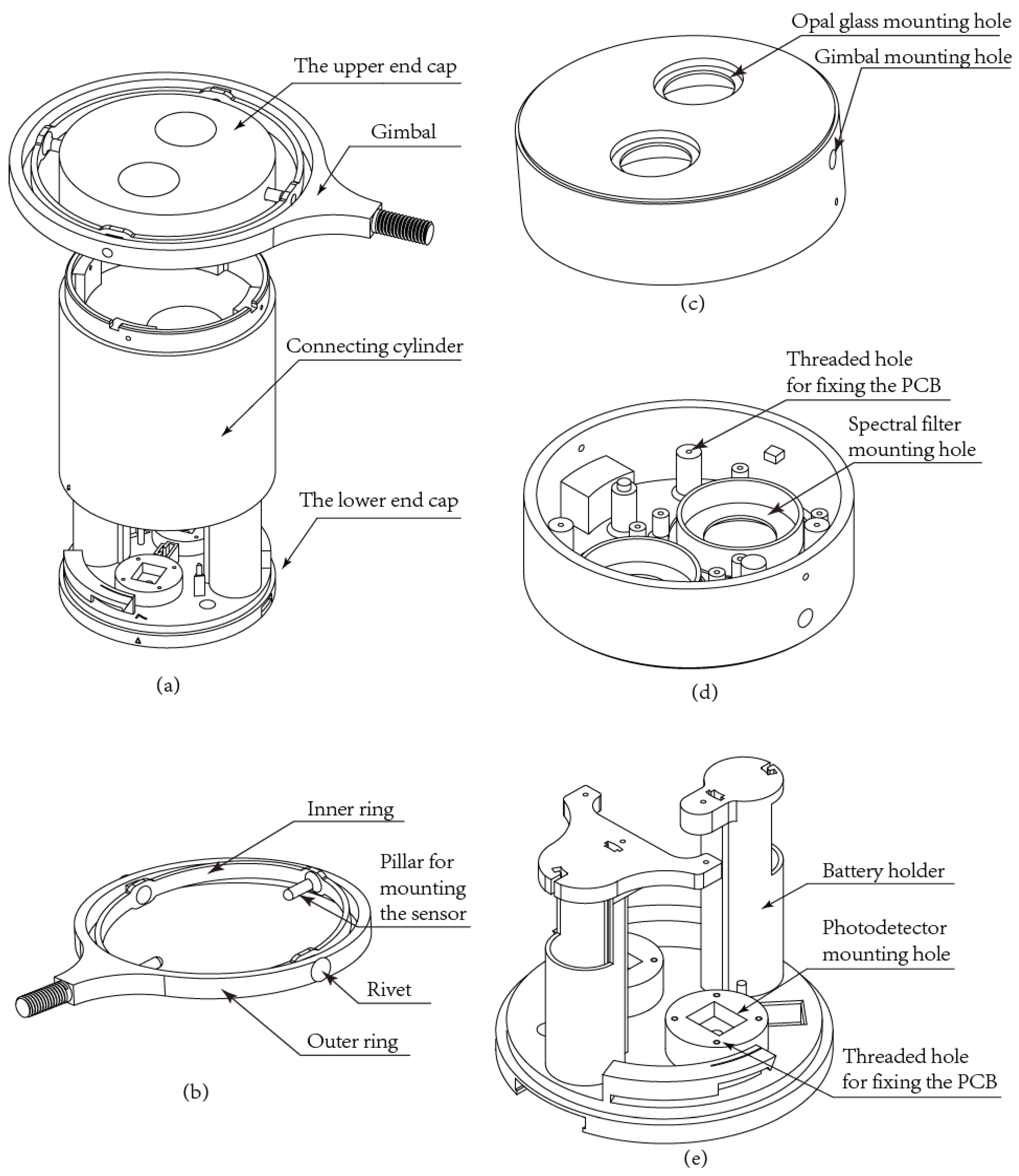
The mechanical components provide support to the optical elements and circuits of the sensor and ensure the operation of the optical path. The mechanical components can be divided into four parts: the upper end cap, the lower end cap, the connecting cylinder, and the gimbal, as shown in Figure 2.
For crop growth information sensors that use direct sunlight as the light source, the upper surface receiving sunlight and the lower surface receiving reflected light from crops are required to be in a horizontal position during operation; otherwise, the measurement accuracy will be affected. The manual method is time-consuming and inefficient. In this study, a gimbal (Figure 2a) that can be mounted on the sensor was designed. The gimbal consists of two rings. The inner ring has a pilar for mounting the sensor. Under the gravity of the sensor, the sensor is able to swing freely to achieve the purpose of automatic balancing.
The upper end cap and the lower end cap are both symmetrical to ensure even distribution of the mass and to facilitate the function of the gimbal. In the upper end cap, there are mounting holes for the opal glass of the cosine corrector, mounting holes for the spectral filter, two gimbal-mounting holes, and pillars for fixing the printed circuit board (PCB), as shown in Figure 2b,c. The height of the PCB-mounting pillars should be appropriate to ensure that after the PCB is installed, the upper surface of the photodetector on the PCB is just next to the filter, and the upper surface of the filter is close to the opal glass. The diameter of the opal glass mounting hole should be much larger than the upper surface of the photodetector to prevent the shadow of the mounting edge of the opal glass entering the photodetector when the sun altitude is low.
The lower end cap is used to house the filters and the batteries. The upper part of the end cap has mounting holes for the photodetector. The diameter and depth of the mounting holes determine the field of view of the sensor. There are threaded holes for fixing the PCB, as shown in Figure 2d. Considering the field application of the sensor, it is more convenient and efficient to use replaceable batteries. The sensor can be operated with two rechargeable 14,500 lithium batteries connected in parallel or two 1.5 V AA batteries connected in series.
3.2. Optical Sensing Unit
The monitoring of different crops or different growth indicators may require spectral information in different bands. For example, RVI at 870 and 660 nm can obtain the LNA of rice and wheat [17]. The NDVI at 730 and 875 nm corresponds to the LAI of wheat [3]. The three-band vegetation index at 924, 703, and 423 nm can estimate the LNC of rice and wheat [18]. The spectral information at 550 and 531 nm can monitor water stress in tomato plants [44]. Therefore, filters with appropriate wavelength bands can be selected according to the types of crops and indicators to be monitored. Our research results indicate that the reflectance spectra at 710 nm and 870 nm are related to the growth information of rapeseed and tomato, and in order to monitor these two crops, we set the spectral bands of the sensor to 710 and 870 nm. The sensor measures the spectral reflectance of the crop canopy at the wavelengths of 710 nm and 870 nm. The optical system of the sensor includes an up-facing unit and a down-facing unit. The up-facing unit receives the incident sunlight on the crop canopy, and the down-facing unit receives the light reflected by the canopy. Each optical channel has a band-pass filter corresponding to the wavelengths. The filter models are FB710-10 and FB870-10 (Thorlabs Inc., Newton, NJ, USA), and the full width at half-maximum (FWHM) is 10 nm. The surface of the filter is smooth glass, and the sunlight is parallel light. When the solar elevation angle is different, the incident angle of the light is different, resulting in the ratio of the sunlight passing through the filter (transmitted energy/incident energy of light at a specific wavelength) to be different. The larger the solar elevation angle, the smaller is the incident angle, the more energy is transmitted, and vice versa. On the contrary, the crop canopy is approximately a Lambertian surface, and the reflected light is diffuse reflection. The energy of the diffuse reflective light passing through the filter is not affected by the solar elevation angle. Thus, the influence of the solar elevation angle on the down-facing unit and up-facing unit is different, which affects the accuracy of the reflectance measurement of the sensor. In order to eliminate the influence of the solar elevation angle on the measurement accuracy, the up-facing unit is equipped with a cosine corrector close to the outer side of the filter. The cosine corrector is an opal glass with rough surfaces on both sides. According to the diameter d of the photosensitive surface of the photodetector, the field of view of the sensor can be determined by setting the length h of the optical channel of the down-facing unit, as shown in Equation (8) and Figure 3. A schematic diagram of the optical sensing unit is shown in Figure 4. The field of view determines the size of the area in which the spectral information of the crop canopy is collected. If the field of view is too small and the crop growth information of the canopy is not consistent, the reflectance measured by the sensor could be less representative, resulting in a large sampling error. Thus, increasing the field of view can improve the accuracy of the measurement. However, at the seedling stage of the crop, before the canopy is big enough to cover the soil between rows, a large field of view may cause the sensor to collect the reflectance spectrum of the canopy and the soil at the same time, leading to inaccurate measurement results. Hence, the field of view needs to be determined properly. Currently, the field of view is often set at about 30°.
The photodetector is responsible for converting the optical signal into an electrical signal. In order to improve the signal-to-noise ratio (SNR) of the sensor, it should have high spectral responsivity to the two wavelengths of the sensor. The photodetector used in this study was an OPT101 (Texas Instruments, Dallas, TX, USA) photodiode. The spectral responsivity at 710 nm and 870 nm was between 0.5 and 0.6 A/W (Figure 5). The dimensions of the photosensitive surface were 2.29 mm × 2.29 mm. The photodiode operated in the photoconductive mode for excellent linearity and low dark current. After the OPT101 was soldered on the PCB, the PCB was covered with black foam to prevent external light from entering the light path.
3.3. Hardware Circuit Design
The sensor works alone and does not form a network with other sensors. The sensor uses WiFi to communicate with a mobile phone or a computer, and is installed with data acquisition software. When the WiFi module receives the acquisition instruction, the sensor collects the light intensity information by adjusting the gain of the photodetector and then converts it into a voltage signal. The analog-to-digital (AD) converter module converts the analog signal into a digital signal. Then, the digital signal is processed to obtain the reflectivity, and the vegetation indices NDVI, RVI, and DVI are further calculated from the reflectivity. The hardware circuit was designed to collect light signals, calculate the reflectance and vegetation index, and communicate with other devices through the wireless module. After the microcontroller unit (MCU) receives the data acquisition command through WiFi, it starts to sequentially collect the output voltage of the OPT101 at the 710 nm up-facing, 710 nm down-facing, 870 nm up-facing, and 870 nm down-facing optical channels. If the voltage is too small, the gain is adjusted to increase the output voltage of the OPT101. If the voltage is saturated, the gain is decreased. The MCU then sends the calculated reflectance and vegetation index to the WiFi module, as shown in Figure 6. The MCU is a 16-bit MSP430G2553 (Texas Instruments, Dallas, TX, USA) microcontroller, which has 1.8–3.6 V low supply voltage, ultra-low power consumption, five power-saving modes, ultra-fast wake-up from standby mode in less than 1 μs, 16-bit reduced instruction set computer architecture, 62.5 ns instruction cycle time, and multiple on-chip peripherals. The power chip is a buck–boost converter TPS63001 (Texas Instruments, Dallas, TX, USA) with a conversion efficiency of up to 96% and an input voltage range of 1.8–5.5 V. The maximum output current is 1200 mA at 3.3 V in the step-down mode, and the maximum output current in the boost mode is 800 mA at 3.3 V. The wireless transmission module is an ESP-12S (Ai-Thinker Technology Co., Shenzhen, China). The ESP-12S communicates with the MCU through a serial port.
The photodiode OPT101 has a single supply, and it is integrated with an operational amplifier, which can realize current-to-voltage (I–V) conversion and output voltage from Pin 5. The OPT101 can use the internal integrated 1 MΩ feedback resistor connecting Pin 4 and Pin 5 or an external feedback resistor between Pin 2 and Pin 5 to obtain different gains (Figure 7). The sensor designed in this study can be used year-round. Since the ambient light intensity varies substantially in different seasons, it is necessary to dynamically adjust the gain of the OPT101 to obtain an appropriate voltage and improve the SNR. In this study, a T-type feedback network was used, and resistors with resistance of tens of kΩ to several hundreds of kΩ were used to obtain amplification above 1 M, thereby avoiding the use of a resistor above 1 MΩ and improving the stability of the circuit (Figure 8). R1, R2, R3, and R4 are precision resistors, and their resistance values are all 39 kΩ. The T-type feedback network uses a TPL0102 (Texas Instruments, Dallas, TX, USA) to adjust the gain of the circuit, which is shown in Equation (9). The TPL0102 is a 256-tap, two-channel digital potentiometer, which has an end-to-end resistance of 100 kΩ, with an I2C communication interface. The AD converter is a 16-bit ADS1118 (Texas Instruments, Dallas, TX, USA) with four single-ended or two differential inputs, an integrated temperature sensor, and an SPI communication interface. ADS1118 consists of an ΔΣ ADC core with eight options for samples per second (SPS); 128 SPS was selected for the sensor. The general-purpose input/output (GPIOs) of the MCU were configured to communicate with ESP-12S, TPL0102, and ADS1118.
where G is the amplification (M); R is the resistance of the TPL0102 (kΩ); and is the sum of the resistance values of the remaining components of the gain circuit.
3.4. Software Design
The software system was designed to collect spectral information and communicate with the WiFi module. In order to ensure stability and low power consumption of the software system as well as the convenience and flexibility of the sensor, the software was developed in the Contiki operating system. Contiki is a lightweight and flexible embedded operating system that was developed at the Swedish Institute of Computer Science [45]. It is event-driven, supports multi-threading, and has minimal requirements for ROM and RAM. Thus, Contiki is very suitable for application in resource-constrained sensors. It has been successfully ported on a variety of MCUs, such as the MSP430 and Atmel AVR. The process code of the Contiki software system is shown in Figure 9. In the software system, when the process is in the state of waiting for an event, the CPU will be released for use by other processes. Only when the event occurs will the process continue to run. When the event processing is completed, the process will re-enter the idle state and release the CPU.
The software system in this study includes processes with a very high frequency of use, such as Initialization, Receives_Serial_Message, Connection, Collecting_Data, and Trans_Message_to_WiFi, as well as processes with a low frequency of use, such as Sampling_Times and Calibration (Figure 10).
- (1)
- The Initialization process is set to AUTOSTART_PROCESSES, which will run automatically when the system is turned on. In the Initialization process, the communication configuration between the MCU and ESP-12S, TPL0102, ADS1118, and other chips as well as the system operation parameters are initialized. After configuring the serial communication parameters with the ESP-12S, the MCU will set the ESP-12S as the TCP Service. If the initialization of the ESP-12S is successful, other processes will be started during the Initialization process, and the started processes will all be in the idle state waiting for events. After initialization is completed, the Initialization process ends automatically. The pseudo code is shown in Algorithm 1.
| Algorithm 1: The pseudo code of the Initialization process |
|
- (2)
- Receives_Serial_Message process. The Contiki operating system broadcasts the WiFi messages received by the serial port through the Serial_Line_Event_Message event. The Receives_Serial_Message process waits for this event and parses the message after receiving the message from the serial port. The parsed content includes the instructions, connection prompts for other devices to connect to WiFi, and WiFi responses when the MCU sends instructions or information to the WiFi module. The instructions mainly include data acquisition, dark-current acquisition, sensor calibration, and number of sampling times. After parsing is completed, the corresponding processes are notified through events. The pseudo code is shown in Algorithm 2.
| Algorithm 2: The pseudo code of the Receives_Serial_Message process |
|
- (3)
- The Connection process waits for the event of other devices connecting to the WiFi module. When the event occurs, the Connection process will send the event to the Trans_Message_to_WiFi process, and the Trans_Message_to_WiFi process will send the sensor ID to the WiFi module. Therefore, other devices that are successfully connected to the sensor will always receive the sensor number. The pseudo code is shown in Algorithm 3.
| Algorithm 3: The pseudo code of the Connection process |
|
- (4)
- The Sampling_Times process waits for the event to set the number of sampling times. Once the event occurs, the received number of times are saved to the flash storage, and the corresponding variable in the program is updated. Then, the event is sent to the Trans_Message_to_WiFi process, which then sends a response to the WiFi module to notify the user. The default number of sampling times for the sensor is 10. The pseudo code is shown in Algorithm 4.
| Algorithm 4: The pseudo code of the Sampling_Times process |
|
- (5)
- The Calibration process waits for the calibration event of the sensor. Once the event occurs, the process saves the received calibration data to the flash storage and then sends the event to the Trans_Message_to_WiFi process. The Trans_Message_to_WiFi process sends a response message to the WiFi module to notify the user that the calibration data have been stored. The pseudo code is shown in Algorithm 5.
| Algorithm 5: The pseudo code of the Calibration process |
|
- (6)
- The Collecting_Data process waits for the data acquisition event. The event includes the COLLECTION command or the DARK command. The DARK command is only used to obtain the dark-current data of the four optical channels of the sensor when the sensor is calibrated. If it is the COLLECTION command, the Collecting_Data process will adjust the gain of the 710 nm and 870 nm OPT101, collect the voltage, and calculate the reflectance and vegetation index. The gain of the OPT101 of the up-facing unit and down-facing unit of the same optical channel is the same. If it is the DARK command, the resistance of the TPL0102 is switched in turn to adjust the gain of the OPT101, and the voltage under different gains is collected. After the COLLECTION command or DARK command is executed, the Collecting_Data process sends the event to the Trans_Message_to_WiFi process, which then sends data to the WiFi module. The pseudo code is shown in Algorithm 6.
| Algorithm 6: The pseudo code of the Calibration process |
|
- (7)
- The Trans_Message_to_WiFi process is responsible for sending response messages or the collected data to the WiFi module. The information that other processes need to send to the WiFi module are all processed by the Trans_Message_to_WiFi process. The pseudo code is shown in Algorithm 7.
| Algorithm 7: The pseudo code of the Trans_Message_to_WiFi process |
|
The sensor communicates externally only through the WiFi module. When the WiFi module receives the instruction information wirelessly, it sends the received information to the serial port of the MCU. The Receives_Serial_Message process deals with the instruction first, and then executes it by the corresponding process. The main commands used to control the sensor are “COLLECTION,” “DARK,” and “Calibration.” The “COLLECTION” command is used when collecting the reflectance and vegetation index, and data collected by the sensor are sent to the WiFi module by the serial port of the MCU. The “DARK” command is used to collect sensor dark-current data. The “Calibration” command is used to calibrate the sensor, and its command format is “Calibration a b,” where “a” and “b” are the calibration coefficients of reflectance at 710 nm and 870 nm, respectively.
4. Calibration and Performance Evaluation of the Sensor
4.1. Calibration
The photodetector generates a photocurrent under illumination; the current is transformed and amplified by the I–V converter circuit to output a voltage; and the magnitude of the output voltage represents the intensity of the illumination. However, one of the inherent characteristics of the photodetector is the dark current, that is, the photocurrent generated in complete darkness. Therefore, the output voltage of the photodetector under a light source consists of the photocurrent and the dark current. The voltage can be calculated using Equation (10):
where is the voltage generated by the direct sunlight and scattered light incident on the sensor; is the output voltage of the sensor; and is the voltage generated by the dark current.
There is a cosine corrector opal glass on the upper surface of the sensor. The irradiance generated by the direct sunlight and scattered light incident on the upper surface of the sensor is (). The relationship between irradiance and voltage is shown in Equation (11):
where (%) is the transmittance of the opal glass; () denotes the ability of the photodetector to convert the light signal to an electrical signal; and () is the photosensitive area of the photodetector. By transforming Equation (11), is obtained:
The output voltage of the sensor when illuminated by the diffuse reflective light of the crop canopy is calculated using Equation (13):
where is the output voltage of the sensor, and is the voltage generated by the dark current.
The relationship between the voltage and the irradiance () generated on the lower surface of the sensor by the diffuse light from the crop canopy is shown in Equation (14):
where () is the photosensitive area of the photodetector. By transforming Equation (14), is obtained:
Based on Equations (7) and (15), the radiant emittance of the crop canopy () is obtained:
where is the half field of view of the sensor, and in this study = . The reflectance of the sensor can be obtained based on Equations (2), (12) and (16):
In reality, the optical components and circuit components are not exactly the same even when they have the same parameters, which will affect the output of the sensor. Moreover, even a slight change in the installation position of the optical components may affect the optical signal. Therefore, it is necessary to use the coefficient to fine-tune . The value of is close to 1; so, the reflectance of the sensor is:
4.2. Calibration Parameters
To calibrate the reflectance of the sensor using Equation (18), we need the voltage generated by the dark current, the transmittance of the cosine corrector, the half field of view of the sensor and . The half field of view of the sensor designed in this study is 15°, and the measured transmittance of the cosine corrector is 47.5%.
At room temperature, the sensor was placed in a dark room. By switching the resistance of the TPL0102 and adjusting the amplification of the four OPT101 components at 710 nm and 870 nm optical channels, the output voltage, that is, the voltage generated by the dark current under different amplification, was measured. The measurement was repeated 40 times, and the relationship between the dark current and the amplification was fitted for each optical channel, as shown in Figure 11. The amplification was calculated according to Equation (9), and the of the sensor used for calibration was 0.1 kΩ. The smaller the resistance value of the TPL0102, the greater the amplification of the OPT101. By switching the resistors from No. 1 to No. 10, the amplification rapidly decreased from 3182 K to 550 K in a nonlinear manner. As the resistor number increased, the decrease in amplification gradually slowed. Hence, the following TPL0102 resistors were selected when measuring the dark current of the sensor: 1–20, 40, 60, 80, 100, 120, 140, and 160, and the range of amplification was 3182–102 K.
At noon on sunny days, 20%, 40%, and 99% standard reflectance gray-scale targets were measured by the sensor, and the output voltage of the sensor was recorded. The measurements were repeated 50 times. During the measurement, the sensor automatically switched the resistance of the TPL0102 to obtain different amplification. The dark current was calculated based on the fitting equations in Figure 11. According to the data of each measurement, can be calculated using Equation (19). Equation (19) can be converted from Equation (18). By taking the average of , can be obtained. The values for the 710 nm and 870 nm channels are calculated separately.
where is the reflectance of the standard reflectance gray-scale target.
From the measurement data, the values for the 710 nm and 870 nm optical channels were 0.97787 and 0.89673, respectively.
4.3. Performance Evaluation of the Sensor
4.3.1. Accuracy Evaluation of the Sensor Using Standard Reflectance Gray-Scale Targets
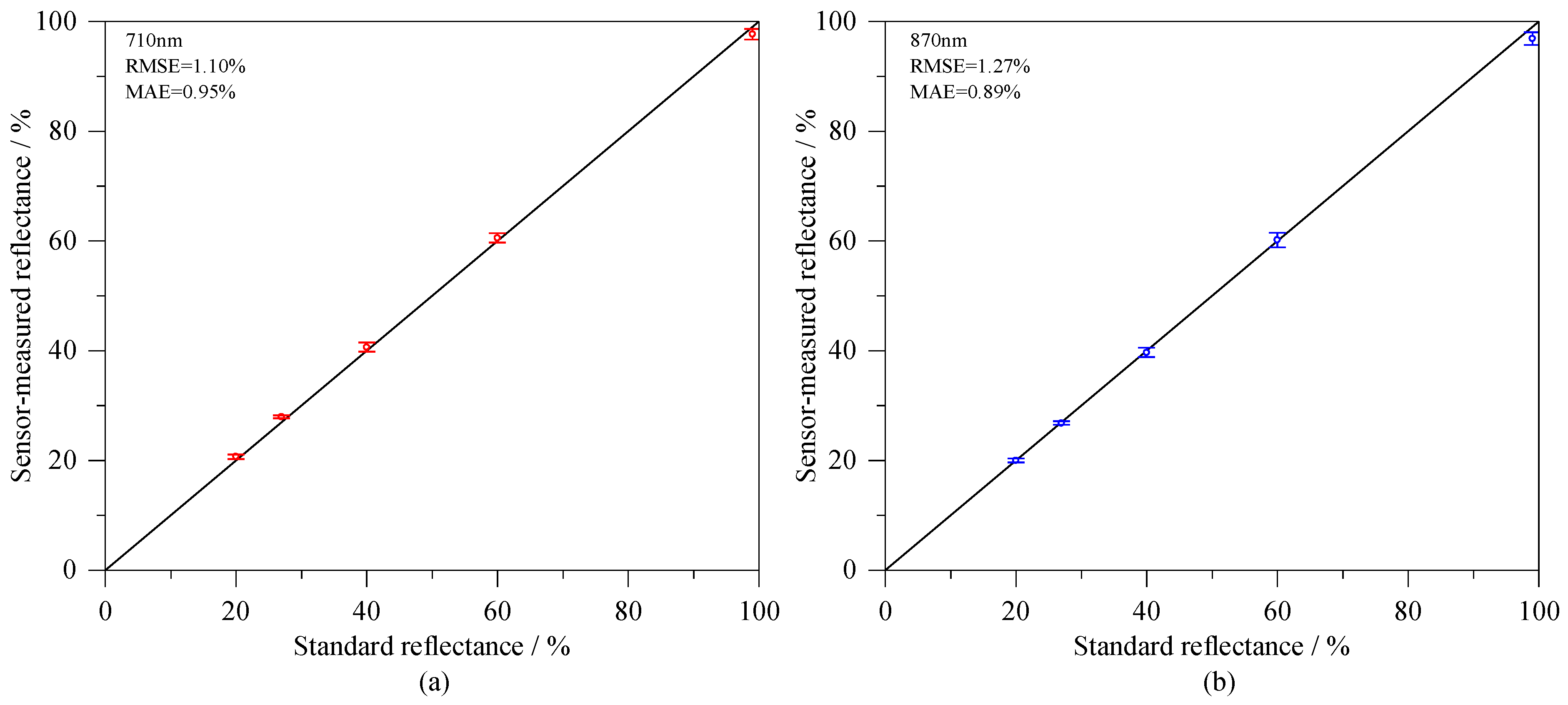
At noon on sunny days, the sensor was used to measure the reflectance of the 20%, 27%, 40%, 60%, and 99% standard reflectance gray-scale targets, and the measurement was repeated five times. The area of gray scale was 255 × 255 mm, the sensor was located just above the gray scale, and the lower surface of the sensor was 200 mm away from the gray scale. Because the sensor’s field of view was 30°, the sensor’s sensing area on the gray scale was a circle with a diameter of about 107 mm. The circular area was completely within the gray scale. The accuracy of the reflectance measured by the sensor was evaluated using the 1:1 graph, root mean square error (RMSE), mean absolute error (MAE), relative error (RE), and coefficient of variation (CV). A 1:1 plot of the measured versus standard reflectance is shown in Figure 12. It can be seen that the reflectance measured by the sensor was very close to the standard reflectance of the gray-scale target, indicating the high accuracy of the sensor. The RMSE at 710 nm and 870 nm bands was 1.10% and 1.27%, respectively, and the MAE was 0.95% and 0.89%, respectively. Figure 13 and Figure 14 show the RE and CV of the reflectance of each standard reflectance gray-scale target measured by the sensor. The RE at 710 nm and 870 nm was within 4% and 3%, respectively, and the CV was between 1% and 2.5%.
4.3.2. Accuracy and Stability of the Sensor under Different Light Intensities
The sunlight intensity at noon gradually increases from spring to summer. On 8 March, 29 March, 21 April, 2 May, 24 May, 5 June, and 17 June 2022, which were sunny and windless days, the reflectance of the 27% standard reflectance gray-scale target was measured at noon to test the accuracy and stability of the measurement under different light intensities. The experiment was conducted at Huaiyin Normal University, Huaian City, Jiangsu Province, China. Each day, five measurement trials were conducted, and the average reflectance was calculated. The results are shown in Figure 15. It can be seen that under different light intensities, the reflectance measured by the sensor had high accuracy. The absolute error was within ±0.5%. The CV of the reflectance at 710 nm and 870 nm was 1.04% and 0.39%, respectively, indicating good stability of the sensor under different light intensities.
4.3.3. Reflectance of Tomato and Rapeseed
With tomato and rapeseed as the measurement objects, the canopy reflectance was measured by the CSRS and ASD spectrometer at 10 farmland plots. During the experiment, the growth periods of tomato and rapeseed were the fruiting period and budding period, respectively, and robust plants were selected for measurement. The CSRS was 40 cm directly above the plant, and the sensed area was a circle with a diameter of about 21.4 cm. The field of view of the ASD was 25°, and to ensure that the perceived area was consistent, we placed the probe of the ASD 48.3 cm above the plant. Because the FWHM of the narrowband filter of the CSRS was 10 nm, in order to ensure comparability of the reflectance measured by the two devices, the reflectance measured by the ASD was processed as follows: the average reflectance at 705–715 nm measured by the ASD was taken as the reflectance at 710 nm, and the average at 865–875 nm was taken as the reflectance at 870 nm. The measurement results are shown in Figure 16. It can be seen that for both tomato and rapeseed, the reflectance measured by the CSRS at 710 nm or 870 nm was close to that of the ASD spectrometer. When tomato was the measurement target, there was a good linear relationship between the NDVI of the CSRS and that of the ASD, and the R2 was 0.9540. When rapeseed was the measurement target, a similar linear relationship was found, and the R2 was 0.9110, as shown in Figure 17.
4.3.4. Automatic Balancing Performance
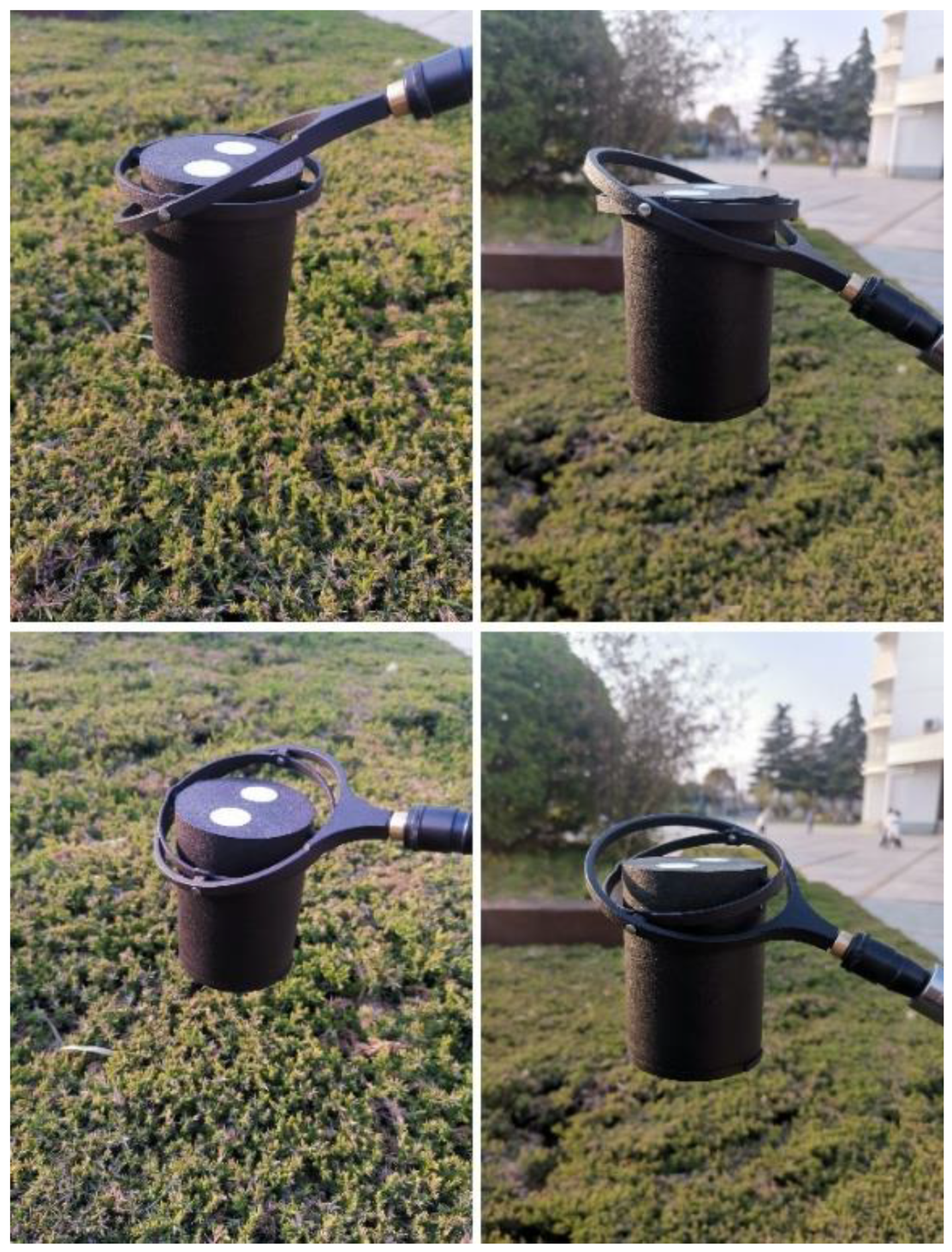
The sensor could be fixed onto a long pole through the screw on the gimbal, which facilitated field measurements. When the height of the measurement object was different, the pitch angle of the pole was different. The automatic balancing function ensured that the central axis of the sensor was always vertical, which improved the efficiency and accuracy of the measurement. Figure 18 shows that the sensor was automatically balanced when the long pole was in different pitch and roll angle positions, indicating that the sensor had a good automatic-balancing performance. In practical applications, the sensor needs to be at a certain height above the plants, which can be achieved by adjusting the inclination of the pole. During the adjustment process, the sensor automatically maintained the balance.
5. Conclusions
- (1)
- In this study, a crop spectral reflectance sensor with automatic posture adjustment was developed. Unlike the current sensors, the balance function was first implemented on a portable sensor, which saves time in sensor balance adjustment and improves work efficiency. The gimbal size is small and requires no power supply to work. It is composed of an inner ring and an outer ring. Under the gravity of the sensor, the gimbal is able to swing freely, such that the central axis is kept in the vertical direction, thereby realizing automatic balancing and improving the efficiency and accuracy of the sensor. The mechanical components of the sensor are arranged symmetrically, such that the mass distribution is balanced to meet the needs of automatic balancing. The field of view of the sensor is 30°; the spectral bands are 710 nm and 870 nm; and the outputs are the reflectance and vegetation index. The sensor is battery-powered and communicates via WiFi. Software was developed for the sensor and the Contiki operating system was used. The photoelectric conversion circuit has 255 combinations of amplifications, ranging from 550 K to 3182 K. Thus, the sensor can work under both strong and weak light intensities.
- (2)
- The paper brings innovation to the research area of sensor calibration methods. Based on the optical signal transmission process and the dark current of the photodetector, the calibration method of the reflectance was theoretically derived, which improved the accuracy of the sensor under different light intensities. The calibration method has good generalizability and can be applied for calibration of other CGISs in the field of smart agriculture. The sensor was then used to measure the reflectance of the 20%, 27%, 40%, 60%, and 99% standard reflectance gray-scale targets. The RMSE of the 710 nm and 870 nm bands was 1.10% and 1.27%, respectively, and the MAE was 0.95% and 0.89%, respectively. The RE was less than 4% and 3%, respectively, and the CV was between 1% and 2.5%. With the 27% standard reflectance gray-scale target as the measurement object, the absolute error of the reflectance measured under different light intensities was within ±0.5%, and the CV at 710 nm and 870 nm was 1.04% and 0.39%, respectively.
- (3)
- With tomato and rapeseed as the measurement objects, the CSRS and ASD spectrometer were used to measure the reflectance of the canopy. The reflectance measured by the CSRS was close to that measured by the ASD spectrometer, and there was a linear relationship between the NDVI of the CSRS and that of the ASD spectrometer. The R2 values for tomato and rapeseed were 0.9540 and 0.9110, respectively. The sensor can also be used in greenhouses, but a skeleton in the greenhouse, such as a galvanized steel pipe, can block the sunlight, which can cause shadows on the crops. Thus, the monitoring area and the upper surface of the sensor should be free of shadows to ensure measurement accuracy.
The technical characteristics of the developed sensor are shown in Table 2.
6. Prospects for Further Research
- (1)
- Now, commercial sensors generally work between 10:00 and 14:00 on sunny days. The circuit of the sensor in this study had a total of 255 kinds of gains, which improved the adaptability of the sensor to strong and weak light intensities of the environment. In the future, we will further study the accuracy of the sensor’s measurement in sunny and cloudy weather, examine the accuracy and stability of the sensor during all-day measurements under these weather conditions, and try to encourage the sensor to work in a variety of weather conditions. On this basis, we will further study the correlation between the vegetation index output by the sensor and the crop growth information.
- (2)
- The gimbal of the sensor in this study had better sensitivity, which could keep the balance of the sensor at all times, and it was suitable for use in conditions with a breeze or without wind. However, when the wind was strong, the gimbal kept swinging, resulting in constant changes in the crop canopy area sensed by the sensor. In further work, we will design a gimbal with a small damping device, so that the sensor can quickly stop when it starts to swing.
- (3)
- The sensor we developed measured the reflectance spectrum of crops, providing reflectance and vegetation indices such as NDVI, RVI, and DVI. When data are saved after the sensor is in use, we will analyze the digitization footprint.
Author Contributions
Conceptualization, N.L., W.Z. and F.L.; methodology, N.L., W.Z. and F.L.; software, N.L. and W.Z.; validation, F.L., M.Z., C.D., C.S. and S.J.; formal analysis, N.L., W.Z., F.L. and J.C.; investigation, N.L., M.Z., C.S., S.J. and H.S.; resources, C.D. and M.Z.; data curation, N.L. and S.J.; writing—original draft preparation, N.L., W.Z. and F.L.; writing—review and editing, N.L. and W.Z.; visualization, N.L., F.L., W.Z. and J.C.; supervision, N.L.; project administration, N.L.; funding acquisition, N.L., W.Z. and C.D. All authors have read and agreed to the published version of the manuscript.
Funding
This work was partially supported by the Natural Science Research Project of Jiangsu Higher Education Institution (18KJA180002, 19KJB170001), National Natural Science Foundation of China (42001296, 31871522), Jiangsu Agricultural Science and Technology Innovation Fund (CX(20)3070); Natural Science Foundation of Jiangsu Province (BK20200277); the Jiangsu Province Key Research and Development Program under Grant BE2020409 (Modern Agriculture); and the Jiangsu Practical Innovation Project for College Students (202110323002, 202110323050H).
Data Availability Statement
The data presented in this study are available from the corresponding author upon reasonable request.
Conflicts of Interest
The authors declare no conflict of interest.
References
- Zhang, J.Y.; Liu, X.; Liang, Y.; Cao, Q.; Tian, Y.C.; Zhu, Y.; Cao, W.X.; Liu, X.J. Using a Portable Active Sensor to Monitor Growth Parameters and Predict Grain Yield of Winter Wheat. Sensors 2019, 19, 1108. [Google Scholar] [CrossRef] [PubMed]
- Sishodia, R.P.; Ray, R.L.; Singh, S.K. Applications of Remote Sensing in Precision Agriculture: A Review. Remote Sens. 2020, 12, 3136. [Google Scholar] [CrossRef]
- Li, H.M.; Lin, W.P.; Pang, F.R.; Jiang, X.P.; Cao, W.X.; Zhu, Y.; Ni, J. Monitoring wheat growth using a portable three-band instrument for crop growth monitoring and diagnosis. Sensors 2020, 20, 2894. [Google Scholar] [CrossRef]
- Gemtos, T.; Fountas, S.; Tagarakis, A.; Liakos, V. Precision Agriculture Application in Fruit Crops: Experience in Handpicked Fruits. Proc. Technol. 2013, 8, 324–332. [Google Scholar] [CrossRef]
- Myers, V.I.; Allen, W.A. Electrooptical Remote Sensing Methods as Nondestructive Testing and Measuring Techniques in Agriculture. Appl. Optics 1968, 7, 1819–1838. [Google Scholar] [CrossRef]
- Bauer, M.E. The Role of Remote Sensing in Determining the Distribution and Yield of Crops. In Advances in Agronomy; Brady, N.C., Ed.; Academic Press: New York, NY, USA, 1975; Volume 27, pp. 271–304. [Google Scholar]
- Shibuyama, M.; Munakata, K. A Spectroradiometer for Field Use: IV. Radiometric prediction of grain yields for ripening rice plants. Jpn. J. Crop Sci. 1986, 55, 53–59. [Google Scholar] [CrossRef]
- Shibuyama, M.; Munakata, K. A Spectroradiometer for Field Use: III. A comparison of some vegetation indices for predicting luxuriant paddy rice biomass. Jpn. J. Crop Sci. 1986, 55, 47–52. [Google Scholar] [CrossRef]
- Shibuyama, M.; Munakata, K. A Spectroradiometer for Field Use: II. Biomass estimates for paddy rice using 1, 100 and 1, 200 nm reflectance. Jpn. J. Crop Sci. 1986, 55, 28–34. [Google Scholar] [CrossRef]
- Wiegand, C.; Shibayama, M.; Yamagata, Y.; Akiyama, T. Spectral observations for estimating the growth and yield of rice. Jpn. J. Crop Sci. 1989, 58, 673–683. [Google Scholar] [CrossRef]
- Shibuyama, M.; Akiyama, T. A spectroradiometer for field use: VI. Radiometric estimation for chlorophyll index of rice canopy. Jpn. J. Crop Sci. 1986, 55, 433–438. [Google Scholar] [CrossRef] [Green Version]
- Shibuyama, M.; Akiyama, T. A Spectroradiometer for Field Use: VII. Radiometric estimation of nitrogen levels in field rice canopies. Jpn. J. Crop Sci. 1986, 55, 439–445. [Google Scholar] [CrossRef]
- Marvin, E.B.; Craig, S.T.D.; Larry, L.B.; Edward, T.K.; Forrest, G.H. Field Spectroscopy of Agricultural Crops. IEEE Trans. Geosci. Remote Sens. 1986, GE-24, 65–75. [Google Scholar]
- Goel, N.S.; Thompson, R.L. Inversion of vegetation canopy reflectance models for estimating agronomic variables. V. Estimation of leaf area index and average leaf angle using measured canopy reflectances. Remote Sens. Environ. 1984, 16, 69–85. [Google Scholar] [CrossRef]
- Shibayama, M.; Akiyama, T. Seasonal visible, near-infrared and mid-infrared spectra of rice canopies in relation to LAI and above-ground dry phytomass. Remote Sens. Environ. 1989, 27, 119–127. [Google Scholar] [CrossRef]
- Ni, J.; Zhang, J.C.; Wu, R.S.; Pang, F.R.; Zhu, Y. Development of an Apparatus for Crop-Growth Monitoring and Diagnosis. Sensors 2018, 18, 3129. [Google Scholar] [CrossRef] [PubMed]
- Zhu, Y.; Yao, X.; Tian, Y.C.; Liu, X.J.; Cao, W.X. Analysis of common canopy vegetation indices for indicating leaf nitrogen accumulations in wheat and rice. Int. J. Appl. Earth Obs. 2008, 10, 1–10. [Google Scholar] [CrossRef]
- Wang, W.; Yao, X.; Yao, X.F.; Tian, Y.C.; Liu, X.J.; Ni, J.; Cao, W.X.; Zhu, Y. Estimating leaf nitrogen concentration with three-band vegetation indices in rice and wheat. Field Crop. Res. 2012, 129, 90–98. [Google Scholar] [CrossRef]
- Cao, Z.S.; Cheng, T.; Ma, X.; Tian, Y.C.; Zhu, Y.; Yao, X.; Chen, Q.; Liu, S.Y.; Guo, Z.Y.; Zhen, Q.M.; et al. A new three-band spectral index for mitigating the saturation in the estimation of leaf area index in wheat. Int. J. Remote Sens. 2017, 38, 3865–3885. [Google Scholar] [CrossRef]
- Tang, Y.L.; Wang, R.C.; Huang, J.F. Relations between red edge characteristics and agronomic parameters of crops. Pedosphere 2004, 14, 467–474. [Google Scholar]
- Pradhan, S.; Bandyopadhyay, K.K.; Sahoo, R.N.; Sehgal, V.K.; Singh, R.; Gupta, V.K.; Joshi, D.K. Predicting Wheat Grain and Biomass Yield Using Canopy Reflectance of Booting Stage. J. Indian Soc. Remote Sens. 2014, 42, 711–718. [Google Scholar] [CrossRef]
- Sun, J.; Shi, S.; Gong, W.; Yang, J.; Du, L.; Song, S.L.; Chen, B.W.; Zhang, Z.B. Evaluation of hyperspectral LiDAR for monitoring rice leaf nitrogen by comparison with multispectral LiDAR and passive spectrometer. Sci. Rep. 2017, 7, 40362. [Google Scholar] [CrossRef] [PubMed]
- Zhang, Y.; Qin, Q.M.; Ren, H.Z.; Sun, Y.H.; Li, M.Z.; Zhang, T.Y.; Ren, S.L. Optimal Hyperspectral Characteristics Determination for Winter Wheat Yield Prediction. Remote Sens. 2018, 10, 2015. [Google Scholar] [CrossRef] [Green Version]
- Pradhan, S.; Sehgal, V.K.; Bandyopadhyay, K.K.; Sahoo, R.N.; Panigrahi, P.; Parihar, C.M.; Jat, S.L. Comparison of Vegetation Indices from Two Ground Based Sensors. J. Indian Soc. Remote Sens. 2018, 46, 321–326. [Google Scholar] [CrossRef]
- Gianquinto, G.; Orsini, F.; Fecondini, M.; Mezzetti, M.; Sambo, P.; Bona, S. A methodological approach for defining spectral indices for assessing tomato nitrogen status and yield. Eur. J. Agron. 2011, 35, 135–143. [Google Scholar] [CrossRef]
- Zhu, Y.; Zhou, D.Q.; Yao, X.; Tian, Y.C.; Cao, W.X. Quantitative relationships of leaf nitrogen status to canopy spectral reflectance in rice. Aust. J. Agr. Res. 2007, 58, 1077–1085. [Google Scholar] [CrossRef]
- Padilla, F.M.; Gallardo, M.; Pena-Fleitas, M.T.; de Souza, R.; Thompson, R.B. Proximal Optical Sensors for Nitrogen Management of Vegetable Crops: A Review. Sensors 2018, 18, 2083. [Google Scholar] [CrossRef] [PubMed]
- Ghazali, M.F.; Wikantika, K.; Aryantha, I.N.; Maulani, R.R.; Yayusman, L.F.; Sumantri, D.I. Integration of Spectral Measurement and UAV for Paddy Leaves Chlorophyll Content Estimation. Sci. Agric. Bohem. 2020, 51, 86–97. [Google Scholar] [CrossRef]
- Cao, Q.; Miao, Y.X.; Shen, J.N.; Yuan, F.; Cheng, S.S.; Cui, Z.L. Evaluating Two Crop Circle Active Canopy Sensors for In-Season Diagnosis of Winter Wheat Nitrogen Status. Agronomy 2018, 8, 201. [Google Scholar] [CrossRef]
- Padilla, F.M.; de Souza, R.; Peña-Fleitas, M.T.; Grasso, R.; Gallardo, M.; Thompson, R.B. Influence of time of day on measurement with chlorophyll meters and canopy reflectance sensors of different crop N status. Precis. Agric. 2019, 20, 1087–1106. [Google Scholar] [CrossRef]
- Ali, A.M.; Ibrahim, S.M.; Bijay-Singh. Wheat grain yield and nitrogen uptake prediction using atLeaf and GreenSeeker portable optical sensors at jointing growth stage. Inf. Process. Agric. 2020, 7, 375–383. [Google Scholar] [CrossRef]
- Ram, H.; Kaur, H.; Sikka, R. Need-based nitrogen management of wheat through use of green seeker and leaf color chart for enhancing grain yield and quality. J. Plant Nutr. 2022, 45, 1–17. [Google Scholar] [CrossRef]
- Debaeke, P.; Rouet, P.; Justes, E. Relationship between the normalized SPAD index and the nitrogen nutrition index: Application to durum wheat. J. Plant Nutr. 2006, 29, 75–92. [Google Scholar] [CrossRef]
- Fernandes, F.M.; Soratto, R.P.; Fernandes, A.M.; Souza, E. Chlorophyll meter-based leaf nitrogen status to manage nitrogen in tropical potato production. Agron. J. 2021, 113, 1733–1746. [Google Scholar] [CrossRef]
- Cui, D.; Li, M.Z.; Zhang, Q. Development of an optical sensor for crop leaf chlorophyll content detection. Comput. Electron. Agr. 2009, 69, 171–176. [Google Scholar] [CrossRef]
- Wang, X.; Zhao, C.J.; Zhou, H.C.; Liu, L.Y.; Wang, J.H.; Xue, X.Z.; Meng, Z.J. Development and experiment of portable NDVI instrument for estimating growth condition of winter wheat. Trans. Chin. Soc. Agric. Eng. 2004, 20, 95–98. [Google Scholar]
- Nie, P.C.; Wu, D.; Yang, Y.; Zhao, K.; He, Y. Development of a portable plant nutrition test instrument based on spectroscopic technique. Afr. J. Microbiol. Res. 2012, 6, 1958–1965. [Google Scholar]
- Yao, L.L.; Wu, R.S.; Wu, S.; Jiang, X.P.; Zhu, Y.; Cao, W.X.; Ni, J. Design and Testing of an Active Light Source Apparatus for Crop Growth Monitoring and Diagnosis. IEEE Access 2020, 8, 206474–206490. [Google Scholar] [CrossRef]
- Lin, L.; He, Y.; Xiao, Z.T.; Zhao, K.; Dong, T.; Nie, P.C. Rapid-Detection Sensor for Rice Grain Moisture Based on NIR Spectroscopy. Appl. Sci. 2019, 9, 1654. [Google Scholar] [CrossRef]
- Tan, C.W.; Wang, D.L.; Zhou, J.; Du, Y.; Luo, M.; Zhang, Y.J.; Guo, W.S. Remotely assessing fraction of photosynthetically active radiation (FPAR) for wheat canopies based on hyperspectral vegetation indexes. Front. Plant Sci. 2018, 9, 776. [Google Scholar] [CrossRef]
- Gilliot, J.; Hadjar, D.; Michelin, J. Potential of Ultra-High-Resolution UAV Images with Centimeter GNSS Positioning for Plant Scale Crop Monitoring. Remote Sens. 2022, 14, 2391. [Google Scholar] [CrossRef]
- Li, S.Y.; Ding, X.Z.; Kuang, Q.L.; Ata-Ul-Karim, S.T.; Cheng, T.; Liu, X.J.; Tan, Y.C.; Zhu, Y.; Cao, W.X.; Cao, Q. Potential of UAV-Based Active Sensing for Monitoring Rice Leaf Nitrogen Status. Front. Plant Sci. 2018, 9, 1834. [Google Scholar] [CrossRef] [PubMed]
- Fahey, T.; Gardi, A.; Sabatini, R. Integration of a UAV-LIDAR System for Remote Sensing of CO2 concentrations in Smart Agriculture. In Proceedings of the 2021 IEEE/AIAA 40th Digital Avionics Systems Conference (DASC), San Antonio, TX, USA, 3–7 October 2021; pp. 1–8. [Google Scholar]
- Ihuoma, S.O.; Madramootoo, C.A. Sensitivity of spectral vegetation indices for monitoring water stress in tomato plants. Comput. Electron. Agr. 2019, 163, 104860. [Google Scholar] [CrossRef]
- Dunkels, A.; Gronvall, B.; Voigt, T. Contiki-a lightweight and flexible operating system for tiny networked sensors. In Proceedings of the 29th Annual IEEE Conference on Local Computer Networks, Tampa, FL, USA, 16–18 November 2004; pp. 455–462. [Google Scholar]
Figure 1.
Appearance of the sensor.

Figure 2.
Structural diagram of the sensor. (a) Exploded diagram; (b) Gimbal; (c) The upper end cap (top view); (d) The upper end cap (bottom view); (e) The lower end cap.
Figure 2.
Structural diagram of the sensor. (a) Exploded diagram; (b) Gimbal; (c) The upper end cap (top view); (d) The upper end cap (bottom view); (e) The lower end cap.

Figure 3.
Schematic diagram of the sensor field of view.

Figure 4.
Schematic of the optical sensing unit.

Figure 5.
(a) OPT101; (b) The spectral responsivity. (Reproduced from Texas Instruments’ datasheet of the OPT101).
Figure 5.
(a) OPT101; (b) The spectral responsivity. (Reproduced from Texas Instruments’ datasheet of the OPT101).

Figure 6.
Overall design of the hardware circuit.

Figure 7.
Gain settings of the OPT101. (a) Using an internal 1 MΩ feedback resistor by connecting Pin 5 and Pin 4; (b) Using an external feedback resistor connecting Pin 5 and Pin 2.
Figure 7.
Gain settings of the OPT101. (a) Using an internal 1 MΩ feedback resistor by connecting Pin 5 and Pin 4; (b) Using an external feedback resistor connecting Pin 5 and Pin 2.

Figure 8.
Diagram of the OPT101 gain adjustment circuit.

Figure 9.
An example of the Contiki process.

Figure 10.
Processes of the software system.

Figure 11.
Dark currents and fitting equations under different amplifications for each optical channel. (a) 710 nm up-facing optical channel; (b) 710 nm down-facing optical channel; (c) 870 nm up-facing optical channel; (d) 870 nm down-facing optical channel.
Figure 11.
Dark currents and fitting equations under different amplifications for each optical channel. (a) 710 nm up-facing optical channel; (b) 710 nm down-facing optical channel; (c) 870 nm up-facing optical channel; (d) 870 nm down-facing optical channel.

Figure 12.
Sensor-measured reflectance vs. standard reflectance. (a) 710 nm; (b) 870 nm.

Figure 13.
Relative error of the reflectance measured by the sensor. (a) 710 nm; (b) 870 nm.

Figure 14.
Coefficient of variation of the reflectance measured by the sensor. (a) 710 nm; (b) 870 nm.
Figure 14.
Coefficient of variation of the reflectance measured by the sensor. (a) 710 nm; (b) 870 nm.

Figure 15.
Reflectance of the 27% standard reflectance gray-scale target measured by the sensor on different dates. (a) 710 nm; (b) 870 nm.
Figure 15.
Reflectance of the 27% standard reflectance gray-scale target measured by the sensor on different dates. (a) 710 nm; (b) 870 nm.

Figure 16.
Crop canopy reflectance measured by the CSRS and ASD spectrometer. (a) Tomato; (b) Rapeseed.
Figure 16.
Crop canopy reflectance measured by the CSRS and ASD spectrometer. (a) Tomato; (b) Rapeseed.

Figure 17.
Fitting curve of the NDVI measured by the CSRS and ASD spectrometer. (a) Tomato; (b) Rapeseed.
Figure 17.
Fitting curve of the NDVI measured by the CSRS and ASD spectrometer. (a) Tomato; (b) Rapeseed.

Figure 18.
Automatic balancing of the sensor.


Table 1.
The characteristics of selected sensors.
| Sensor/Spectrometer | Active/Passive Light Source | Bands | Size | Automatic Balancing | Portable | Application Field |
|---|---|---|---|---|---|---|
| FieldSpec FR spectroradiometer | Passive | 350–2500 nm | 127 × 368 × 292 mm | No | No | Scientific research |
| MSR16 | Passive | 16 bands, 460–1700 nm | 80 × 80 × 100 mm | No | No | Scientific research |
| MSR87 | Passive | 460, 510, 610, 660, 710, 760 and 810 nm | 80 × 80 × 100 mm | No | Yes | Scientific research |
| MSR5 | Passive | 485, 560, 660, 830 and 1650 nm | 80 × 80 × 100 mm | No | Yes | Scientific research |
| Crop Circle ACS-470 | Active | 450, 550, 650, 670, 730, and 760 nm | 201 × 89 × 48 mm | No | Yes | Scientific research |
| GreenSeeker crop sensing system | Active | 656 and 774 nm | 277 × 86 × 150 mm | No | Yes | Scientific research/agricultural application |
| GreenSeeker handheld crop sensor | Active | 660 and 780 nm | 90 × 270 mm | No | Yes | Scientific research/agricultural application |
| SPAD-502 | Active | 650 and 940 nm | 78 × 164 × 49 mm | NA | Yes | Scientific research |
| Optical sensor to monitor the chlorophyll content [35] | Passive | 610 and 1220 nm | 105 × 54 × 124 mm | No | Yes | Scientific research/agricultural application |
| CGMD [16] | Passive | 720 and 810 nm | 44 × 44 × 52 mm | No | Yes | Scientific research/agricultural application |
| Plant nutrition test instrument [37] | Active | 650 and 940 nm | about is a palm size | No | Yes | Agricultural application |
Table 2.
The characteristics of the developed sensor.
| Active/Passive Light Source | Bands | Size | Automatic Balancing | Portable | Application Field |
|---|---|---|---|---|---|
| Passive | 710 and 870 nm | 71 × 71 × 99 mm | Yes | Yes | Scientific research/agricultural application |
Publisher’s Note: MDPI stays neutral with regard to jurisdictional claims in published maps and institutional affiliations. |
© 2022 by the authors. Licensee MDPI, Basel, Switzerland. This article is an open access article distributed under the terms and conditions of the Creative Commons Attribution (CC BY) license (https://creativecommons.org/licenses/by/4.0/).
Share and Cite
MDPI and ACS Style
Liu, N.; Zhang, W.; Liu, F.; Zhang, M.; Du, C.; Sun, C.; Cao, J.; Ji, S.; Sun, H. Development of a Crop Spectral Reflectance Sensor. Agronomy 2022, 12, 2139. https://0-doi-org.brum.beds.ac.uk/10.3390/agronomy12092139
AMA Style
Liu N, Zhang W, Liu F, Zhang M, Du C, Sun C, Cao J, Ji S, Sun H. Development of a Crop Spectral Reflectance Sensor. Agronomy. 2022; 12(9):2139. https://0-doi-org.brum.beds.ac.uk/10.3390/agronomy12092139
Chicago/Turabian StyleLiu, Naisen, Wenyu Zhang, Fuxia Liu, Meina Zhang, Chenggong Du, Chuanliang Sun, Jing Cao, Shuwen Ji, and Hui Sun. 2022. "Development of a Crop Spectral Reflectance Sensor" Agronomy 12, no. 9: 2139. https://0-doi-org.brum.beds.ac.uk/10.3390/agronomy12092139
Note that from the first issue of 2016, this journal uses article numbers instead of page numbers. See further details here.