
A Remote-Sensing-Assisted Estimation of Water Use in Rice Paddy Fields: A Study on Lis Valley, Portugal


1
Instituto de Desarrollo Regional, UCLM Universidad de Castilla-La Mancha, 02071 Albacete, Spain
2
IPC Instituto Politécnico de Coimbra, Escola Superior Agrária de Coimbra, 3045-093 Coimbra, Portugal
*
Author to whom correspondence should be addressed.
Agronomy 2023, 13(5), 1357; https://0-doi-org.brum.beds.ac.uk/10.3390/agronomy13051357
Submission received: 6 April 2023
/
Revised: 3 May 2023
/
Accepted: 9 May 2023
/
Published: 12 May 2023
(This article belongs to the Special Issue Water Saving in Irrigated Agriculture)
Abstract
:Rice culture is one of the most important crops in the world, being the most consumed cereal grain (755 million tons in 2020). Since rice is usually produced under flooding conditions and water performs several essential functions for the crop, estimating its water needs is essential. Remote sensing techniques have shown effectiveness in estimating and monitoring the water use in crop fields. An estimation from satellite data is a challenge, but could be very useful, in order to spatialize local estimates and operationalize production models. This study intended to derive an approach to estimate the actual crop evapotranspiration (ETa) in rice paddies from a temporal series of satellite images. The experimental data were obtained in the Lis Valley Irrigation District (central coast of Portugal), during the 2019 to 2021 rice growing seasons. The average seasonal ETa (FAO56) resulted 586 ± 23 mm and the water productivity (WP) was 0.47 ± 0.03 kg m−3. Good correlations were found between the crop coefficients (Kc) proposed by FAO and the NDVI evolution in the control rice fields, with R2 ranging between 0.71 and 0.82 for stages II+III (development + middle) and between 0.76 and 0.82 for stage IV (late). The results from the derived RS-assisted method were compared to the ETa values obtained from the surface energy balance model METRIC, showing an average estimation error of ±0.8 mm d−1, with a negligible bias. The findings in this work are promising and show the potential of the RS-assisted method for monitoring ETa and water productivity, capturing the local and seasonal variability in rice growing, and then predicting the rice yield, being a useful and free tool available to farmers.
1. Introduction
Rice is often recognized as the most important human food crop, as it is responsible for feeding more than half of the human population, being the most consumed cereal grain [1]. Its leading producer is China, whose average annual production was 210 million tons between 2011 and 2020. In the last decade, the production of rice has grown nearly 61 million tons, from 694 million to 755 million tons, while its harvested area has increased by 2 million ha [2]. In Portugal, rice is mainly grown in the lower valleys of the rivers Sorraia, Tejo, Sado, and Mondego, but also in other regions on a smaller scale, such as the Lis Valley Irrigation District (LVID). The national cultivated rice area exceeded 30,000 ha in 2021, with a production of nearly 173,000 tons [3]. A large amount of the rice produced in Portugal is oblong grain, called carolino (Oryza sativa L. ssp. indica), but agulha rice (Oryza sativa L. ssp. japonica) is also produced, with a characteristically elongated grain.
Water has a fundamental role in rice culture: (i) it allows the satisfaction of physiological needs (the growth and development of the crop); (ii) it acts as a thermal regulator—it is the most evident and important thermal protection in the initial phase of the cycle and flowering; (iii) it assists in weed control; (iv) it facilitates the availability of nutrients; and (v) it promotes the leaching of salts [4,5,6]. Traditional irrigation is performed by a continuous flooding method in level basins, which is very demanding for water in comparison with most methods applied to other crops. Overall, rice crop needs about 1100–1500 mm of water [7,8] during the growing period, which is considered high when compared to other grain crops. The reason for this is that other components of water use besides evapotranspiration (water evaporation plus plant transpiration) are taken into account, such as percolation (the vertical movement of water in the soil beyond the root zone), lateral flow losses, and surface drainage. When only evapotranspiration is considered, the rice’s water use efficiency is comparable to that of other cereals [9,10].
According to the methodology suggested by the Food and Agricultural Organization of the United Nations (FAO), crop water requirements are commonly calculated by multiplying the reference evapotranspiration (ETo) by the crop coefficient (Kc) to estimate the actual evapotranspiration (ETa) of a particular crop [11]. At field scale, ETa is important for planning efficient irrigation systems, being an integral part of field management decision support tools. Additionally, the estimation of ETa allows for an understanding of the hydrological cycle, which is directly affected by global climate change [12]. Some studies have focused on the determination of Kc using the ET measured from crops with experimental methods. Specifically, for rice, published studies include lysimeters [13], Bowen ratio energy balance [14], and eddy covariance [15]. These alternative methods can be used over relatively small areas but are difficult to extrapolate in time and space given heterogeneous land surfaces [16] and crop, soil, and weather variations [17]. Due to these limitations, several remote sensing (RS)-based models and algorithms have been developed to quantify the ETa in rice, complementing the agrometeorological data observed on the ground and providing more detailed spatial information. Most of them are based on the surface energy balance, e.g., the Simplified Surface Energy Balance Index (S-SEBI) [18], Surface Energy Balance Algorithm for Land (SEBAL) [19], and Mapping Evapotranspiration at High Spatial Resolution with Internalized Calibration (METRIC) [20]; other models couple biophysical parameters and energy balance, e.g., the Breathing Earth System Simulator (BESS) [21], while others combine carbon and vapor fluxes through the response of the canopy conductance to the photosynthesis rate (PML-V2) [22], or integrate earth observations (i.e., the MODIS surface reflectance, albedo, and daily ground surface climate datasets) and numerical algorithms to calculate the ETa [23].
The Kc values represent the integrated effects of changes in the leaf area, plant height, crop characteristics, irrigation method, rate of crop development, crop planting date, degree of canopy cover, canopy resistance, soil and climate conditions, and management practices [24]. Single and dual crop coefficient approaches have been widely used. The single crop coefficient combines the impact of the transpiration from the crop with the evaporation from the soil in a single coefficient [25], whereas the dual crop coefficient represents Kc as the sum of the basal crop coefficient (Kcb) with the transpiration and soil evaporation coefficient (Ke), representing the evaporation from the soil surface. According to Allen et al. [11], the single crop coefficient is used for irrigation planning and design, irrigation management, and the basic and real-time irrigation scheduling of less frequent water applications, while the dual crop coefficient is mainly used in research and for real-time irrigation scheduling, the irrigation scheduling of highly frequent water applications such as daily irrigation, supplementary irrigation, and detailed soil and hydrologic water balance studies. These authors presented the crop coefficients of various crops under unlimited irrigation conditions, using both single and dual crop approaches, but explaining that Kc can be affected by the evaporation from soil, crop type, weather conditions (i.e., precipitation, wind speed, and relative humidity), and crop growth [26]. Most of the literature (e.g., [11,26]) calculates the rice ETa using the single crop coefficient approach (ETa = Kc × ETo), an understanding shared by the authors of this paper. The dual crop coefficient approach is better applied for crops that do not occupy the entire surface of the soil (e.g., orchards, more spaced vegetables, or cover crops). For arable crops with a higher density, the single crop coefficient approach is preferable. The added value of dual Kc is to obtain details on the evaporative component, which is minimized if crops produce a high soil shading (due to a higher density). Dual Kc makes it possible to value the evaporation that occurs right after rain or irrigation (mainly by sprinklers), where the surface is wet and exposed to the sun. After a few days, the evaporation practically ceases, as soon as the evaporative layer (about 10 cm deep) is free of water. None of this applies to rice, because the surface is wet from sowing, and even in the intermediate breaks without flooding, the soil surface remains very wet. Late in the cycle, the soil surface gets drier, but then the crop shades the surface.
The RS approach has been used as an alternative for the calculation of Kc, in particular through the use of vegetation indices (VI’s) derived from satellite data. The Normalized Difference Vegetation Index (NDVI) is one of the most widely used vegetation indices in agriculture. Although the NDVI can be affected by the saturation effect and soil reflectance [27], the main reason for choosing this index is to give continuity to the previous works reported in the literature [28,29]. This index benefits from the characteristics of two spectral bands: the chlorophyll pigment absorptions in the red spectral band (0.62–0.69 μm) and the high reflectance of plant materials in the NIR band (0.75–1.3 μm) [30]. The index is calculated as the normalized ratio between the red and NIR wavelength bands, as (NIR − RED)/(NIR + red) [31,32]. The NDVI ranges from −1 to 1, and, since high photosynthetic activity leads to lower values of reflectance coefficients in the red region of the spectrum and large values in the NIR region, the ratio between these indicators allows for a clear separation of vegetation from other natural elements. A bare soil usually has an NDVI value of 0.1 to 0.2, while the vegetation has indices between 0.2 and 1, because plants have a low reflectance in the red band and a strong NIR reflectance [33]. The NDVI is directly related to the plants’ photosynthetic capacity energy absorption of plant canopies and allows for an observation of the vegetation dynamics throughout the growing season [34] and an estimation of the crop yield, in combination with other parameters [35], detecting problematic areas within the plot (related to soil, sowing, or irrigation issues, as well as in terms of the presence of weeds, pests, or diseases). The onset of Kc(b)-VI approaches for estimating crop coefficients relies on the similarities between the curves of Kc (and Kcb) and the VI’s. Overall, wide acceptance of the Kc(b)-VI approaches for estimating crop coefficients has occurred in recent decades. Regarding the studies applied to rice, some authors have developed a satellite-based Kc for an estimation of ETa,, validating the results using the latent heat flux observed from a flux tower. These authors concluded that the Kc produced a reasonable estimation of the ETa [36]. In another study, the Kc was estimated using four methods, including the linear relationship between Kc and VI, a calibrated model of Kc-VI, the linear relationship between Kcb and VI, and a calibrated model of Kcb-VI using Landsat 7 images. The results showed that the changes in Kc were well explained by the changes in the NDVI in all the methods [37]. Other studies were performed on crops such as wheat [38,39], maize [40], sorgum [41], and grapes [42]. The overall conclusion of these studies was the great strength of the reflectance-based models from the point of view of crop irrigation management. Within this scope, some operational tools have been developed to integrate a time series of satellite information into an RS assistance of the FAO 56 methodology for a determination of the surface water availability of plants. For instance, the HidroMORE© platform, developed by the University of Castilla-La Mancha, Spain, implements the retrieval of the basal crop coefficients (Kcb) through the dependence of NDVI-Kcb [43]. This operational tool has been applied in several studies [44,45], including water accounting on the Water Users’ Association (WUA) management scales [46,47].
The main objective of this study was to derive an approach to determine the ETa in rice paddies from a temporal series of satellite NDVI images, provided by SPIDERwebGIS© from the University of Castilla-La Mancha, Spain, making possible to obtain a process that can be extensively applied to improve irrigation and crop management. An assessment of this approach was conducted, comparing these results with the ETa results from METRIC in the study site in Lis Valley. To our knowledge, this is the first report of a study in which the ETa provided by the METRIC platform was compared with the ETa calculated using the FAO56 methodology, concluding the success of this tool for rice. Therefore, this paper also intends to demonstrate that both tools are reliable and allow for consulting the data provided from RS in an accessible and user-friendly way.
2. Materials and Methods
2.1. Description of the Study Site and Agronomic Management of the Rice
This study was conducted in the Lis Valley Irrigation District (LVID) throughout three growing seasons, from 2019 to 2021. LVID is a public irrigation district located in the Administrative District of Leiria (Central Coast of Portugal). The climate is Cbs type (Köppen climate classification) and characterized by temperate summers and winters with mild temperatures. Its precipitation is concentrated mainly from October to March and the average values of this decrease from the headwaters of the Lis Valley basin towards the coastal region. Its annual average temperature is 15.9 °C and annual average precipitation is 790 mm [48]. Rice represents 8.3% of the irrigated area [49] and is grown in traditional rice paddies in an area of around 140 ha, cultivated by two familiar enterprises (Figure 1).
The experiments focused on a paddy field, identified as P1 (Plot 1) (N 39°52′22.188″, W 8°52′58.606″), with an area of 3 ha (215 m × 140 m). The soil was clayey, with 7.11% sand, 37.32% silt, and 55.58% clay, and an average root zone depth of 40 cm. The soil had a content of 2.7% of organic matter and a pH of 7.2. The soil electrical conductivity (EC) was 0.59 mS cm−1, which indicates a very low salinity. The field capacity was 0.385 cm3 cm−3 and the wilting point was 0.204 cm3 cm−3. The nitrogen, according to the Kjeldahl method, was 0.16%. The farmer used a soil fertilization scheme supported by soil analyses. As a reference, in 2020, the base fertilization of N-P-K was applied at 15-15-15% (190 kg/ha), while the top dressing fertilization was 20-20-0% (200 kg/ha). Irrigation was applied via continuous flooding, powered by derivation from a surface ditch. The water table varied from 0.75–0.85 m from the ground surface. The drainage conditions were reasonable and the infiltration conditions in the soil were low. Three additional rice plots, adjacent to P1 and owned by the same farmer, were also used for validation.
The frequency of the irrigation in the plots was variable, in a system that Portuguese rice farmers call “ir às regas”, which means that the bed is completely filled, left, and only filled again when the water table is very low. In terms of practical effects, this means that the dry period is almost non-existent, except for the time when herbicides are applied and when the harvest is close (usually between the last 22–25 days). The measurements of the inflow and outflow discharges in P1 were measured using automatic water level sensors, where the data were complemented with the measurement of the atmospheric pressure through a barometer located nearby (Table 1), following the methodology used by Gonçalves et al. [50] (Figure 2a). The sensors were inserted into a water tube consisting of a PVC pipe and placed on soil at a 25 cm depth. The data were periodically downloaded with a portable docking station.
Before sowing, rice seeds go through a process called “plunging”, whereby the bags are immersed in water for a period of 24 to 48 h. Because of their water absorption, the seeds increase in volume and become heavier, which prevents them from floating after being seeded in paddy fields. For the embryo to germinate, the water in the seedbeds must be kept for about a week, allowing for the growth of rootlets to be able to “cling” to the soil. At this point, the water is removed slowly via surface drainage to avoid dragging the seeds, thus promoting their rooting and the subsequent development of the plant. In the sowing of this rice, the farmer used a combination of “Luna”, “Teti”, and “Lusitano” seeds in varying amounts. To obtain the rice yield, 5 sampling points were chosen to spatially represent the entire P1 plot, crosswise, from which a 0.5 m2 (100 cm × 50 cm) sample was taken, following the methodology used by Gonçalves et al. [50] (Figure 2c) in a procedure that is commonly used in rice experimentation in Portugal. All the sampled plants were collected manually. The dry biomass measurement included the whole plant (leaves, panicles, stems, and grain), excluding the roots. The parameters analyzed were the entire grain at 14% humidity, the average grain weight (weight of 1000 grains), the straw, and the total biomass. The same procedure was repeated from 2019 to 2021, which made it possible to collect a total of 15 samples.
The availability of irrigation and crop yield data allow for a calculation of WP, which is generally defined as the crop yield per cubic meter of water consumption, including the effective precipitation and diverted water from water systems for irrigated areas. The WP (kg m−3) was computed by dividing the yield (kg ha−1) by the amount of total water applied (precipitation plus irrigation) (m3 ha−1).
During vegetative development, weeds compete with rice plants for water, light, nutrients, and space, besides serving as hosts for pests and diseases. The treatments were carried out with plant protection products, observing the principles of integrated production. The active substances applied were aimed at combatting broad-leafed weeds (e.g., Heteranthera limosa), but also cyperacae and grasses, such as Cyperus difformis and Echinochloa spp. The more frequent diseases are caused by two fungi: Pyricularia oryzae and Helminthosporium oryzae. Regarding the crop pests more often detected, the Lousiana red crayfish (Procambarus clarkii) is the most worrisome, which, being an omnivorous freshwater crustacean, is a consumer of rice plants in its adult stage, especially during the early stages of the rice. The presence of aquatic birds, such as storks and herons, which feed on the crayfish, brings benefits to its control, but causes irreparable damage to the growth of rice plants, which become stunted.
2.2. Weather Station, Reference and Actual Evapotranspiration through the FAO56 Methodology
The weather conditions during the three study seasons were measured from an automated agrometeorological station (N 39°52′37.66″, W 8°53′26.919″), located at a distance of 0.8 km from P1 (Figure 2b). All the sensors were installed at a height of 2 m above the grass surface and meteorological data were registered hourly (Table 2). The variables measured were: air temperature, relative humidity, wind speed, wind direction, daily average incoming solar radiation, and precipitation.
The first approach to the rice actual evapotranspiration, ETa, was obtained following the FAO-56 concept (ETa = Kc × ETo) [51]. The daily ETo values were calculated using the FAO56 Penmann–Monteith reference ET equation for grass [11]:
where ETo is the reference evapotranspiration (mm d −1), Rn is the net radiation (MJ m−2 d −1), G is the soil heat flux density (MJ m−2 d −1), T is the air temperature at a 2 m height (°C), u2 is the wind speed at a 2 m level (m s−1), es is the saturation vapor pressure of the air (kPa), ea is the actual vapor pressure (kPa), Δ is the slope vapor pressure curve (kPa °C−1), and γ is the psychrometric constant (kPa °C−1).
The lengths of the rice growth stages were identified from Table 11 of the FAO-56 manual (reference) (I—initial, II—development, III—middle, and IV—late), choosing a cycle of 150 days, sowed in May, corresponding to the rice agricultural management in the LVID (Table 3). The crop coefficient for the initial stage (Kcini) was obtained from the sub-section of the FAO-56 about paddy rice (Table 14, [11]), applying the value for a sub-humid to humid climate, under a light to moderate wind speed. The crop coefficients for the mid-season and late-season stages (Kcmid and Kclate, respectively) were adjusted to the conditions of the local site, as the minimum relative humidity (RHmin) was higher than 45% and the average wind speed (u2) sometimes exceeded 2.0 ms−1 in 2020, as follows:
where Tab is the value in Table 12 [11] for the rice crop, u2 is the wind speed at a 2 m level (m s−1), and h is the maximum height of the crop, also obtained from the same table.
2.3. Actual Evapotranspiration from METRIC
Twenty clear-sky Landsat 8 images (6 in 2019, 7 in 2020, and 7 in 2021) were available for the study site (Table 4). Cloud-free images were selected to cover the period of time between the sowing and harvest of each growing season. The images were processed on the EEFlux platform version 0.20.4 (https://eeflux-level1.appspot.com, accessed on 15 January 2022). EEFlux is a fully automated framework for METRIC that operates on the Google Earth Engine platform to derive RS-based ET estimates using the METRIC algorithm [52]. The application deploys Landsat’s thermal and shortwave bands to derive the ETa from the albedo, vegetation index, land surface temperature, and other surface parameters [53]. The images in the METRIC-EEFlux were internally calibrated from the alfalfa ETo, using gridded weather data to retrieve the fraction of the ETo (EToF). This fraction was used to extrapolate the instantaneous ET (ETins), which represents the ET at each pixel at the time of the satellite overpass, derived from the latent heat flux as:
where ETins is the instantaneous ET (mm h−1), LE is the latent heat flux (W m−2), ‘λ’ is the latent heat of vaporization (J kg−1), and ρ is the density of water (kg m−3). The fraction of the reference ET is computed as:
ETins = 3600 × (LE/λ × ρ)
EToF = ETinst/EToinst
The daily ETa at each pixel is derived as:
ETa = EToF × ETo
Since the spatial resolution of 30 m allows for the allocation of several pixels within the plots, the mean values for the 3 × 3 pixels were extracted using the QGis software (version 3.18.3 Zurich) for image processing.
2.4. Satellite Acquisition and Ground Meaurements of NDVI
To obtain the NDVI, the satellite imagery from the constellation Landsat 8 (USGS) and Sentinel-2A and 2B (UE Copernicus Program) was explored. Sentinel-2 has a revisit frequency of 5 days at the Equator and provides VNIR data with a spatial resolution of 10–20 m. Landsat 8 has a temporal resolution of 16 days and its Operational Land Imager (OLI) sensor provides images at a 30 m spatial resolution (visible, NIR, and SWIR), whereas the TIRS sensor provides thermal data at a spatial resolution of 100 m in two thermal bands. Landsat 9 was recently launched (September 2021), increasing the revisit time for the Landsat data collection. The path/row for Landsat is 204/32 and for Sentinel-2 is “TILE29TNE”.
The platform SPIDERwebGIS© (http://maps.spiderwebgis.org/webgis/, accessed on 30 May 2022), henceforth SPIDER, developed by the University of Castilla-La Mancha in Spain, was used for the management of the satellite image datasets. The Orthorectified Surface Reflectance (Bottom-Of-Atmosphere: BOA) imagery was considered, i.e., the images were atmospherically corrected in order to eliminate or compensate for the effects of atmospheric elements on the image, thus obtaining a comparable surface signal for the areas and different acquisition dates.
The feature that differentiates this platform is its capability to graphically display the temporal evolution of surface reflectance, VIs, or water requirements, among other options. The data can be analyzed through both the time series of interactive charts that allow for users to predefine query parameters and date ranges, or can be exported to standard spreadsheet formats. The 4 rice plots were identified in SPIDER and a sample of 5 points within each plot limits was chosen for the 2019–2021 growing seasons, covering the time between sowing and harvesting. The average of the 5 sampling points was calculated for a more reliable result. For the dates when satellite images were not available, the NDVI was linearly interpolated between the time-adjacent satellite images to obtain the continuous temporal evolution of the NDVI at a daily scale.
For the assessment of the satellite estimates of this key input, the field measurements of the NDVI were conducted in the 2020 campaign in eight transects within P1 using a GreenSeeker Handheld Crop Sensor (Figure 2d), and were used as ground truth. Since most of the time the soil remained flooded, an extensor was needed to measure further inside the field, minimizing the effect of the path on the satellite images and plant growth. The sensor was handheld over the canopy at an average height of 1 m above the crop and the existence of a remote switch allowed for capturing the NDVI measures with precision.
3. Results
3.1. Meteorological Data
Table 5 shows the meteorological data for each month from the 2019 to 2021 rice growing seasons (May–October). The monthly averages of the air temperature ranged between 14.4 and 19.7 °C and the wind speed ranged between 1.4 and 2.7 m s−1. The cumulative precipitation resulted 178.7 mm in 2019, 214.2 mm in 2020, and 258.8 mm in 2021, mainly concentrated in September–October, although both May 2020 and 2021 were considerably rainy. Namely, in 2021, it is important to note that severe weather phenomena were recorded between June 11 and June 20, including the occurrence of heavy precipitation accompanied by hail, thunderstorms, and strong convective wind gusts. Overall, both growing seasons in the site were typical of the average weather conditions on the central coast of Portugal, although the precipitation in the three periods was below normal records [54,55,56]. In terms of temperature, the summer of 2019 was cold and dry (the average minimum air temperature was the lowest in the last 40 years, with June being the coldest since 2000) [54]. In 2020, hot periods were registered in May, July (the hottest since 1931), and September (occurrence of a heatwave) [55]. The summer of 2021 was considered to be normal in terms of air temperature and dry in terms of precipitation. The average temperature for the month of May 2021, lower than that recorded in the corresponding months of 2019 and 2020, reflected the very low minimum temperature values, which were almost always lower than the average monthly values [56]. The monthly averages of the relative humidity were especially high in May and June of 2020 and 2021 when compared to the same period in 2019. As a consequence, the average evapotranspiration demand was higher in 2020 and 2021 than in 2019, which was especially noticed in July.
3.2. Evapotranspiration, Crop Coefficients and Water Use
The rice campaign in 2019 occurred between 23 May and 22 October (153 days); in 2020 between 14 May and 10 October (149 days); and in 2021 between 19 May and 11 October (146 days). These dates refer to sowing and harvest, respectively, without major differences in the four selected plots. Although the 2019 rice growing season was longer, the ETo was higher in 2020, mainly due to the higher evaporative demand and drier conditions during the middle stage (Table 6). The 2021 campaign was the shortest, but with the lowest evaporative demand.
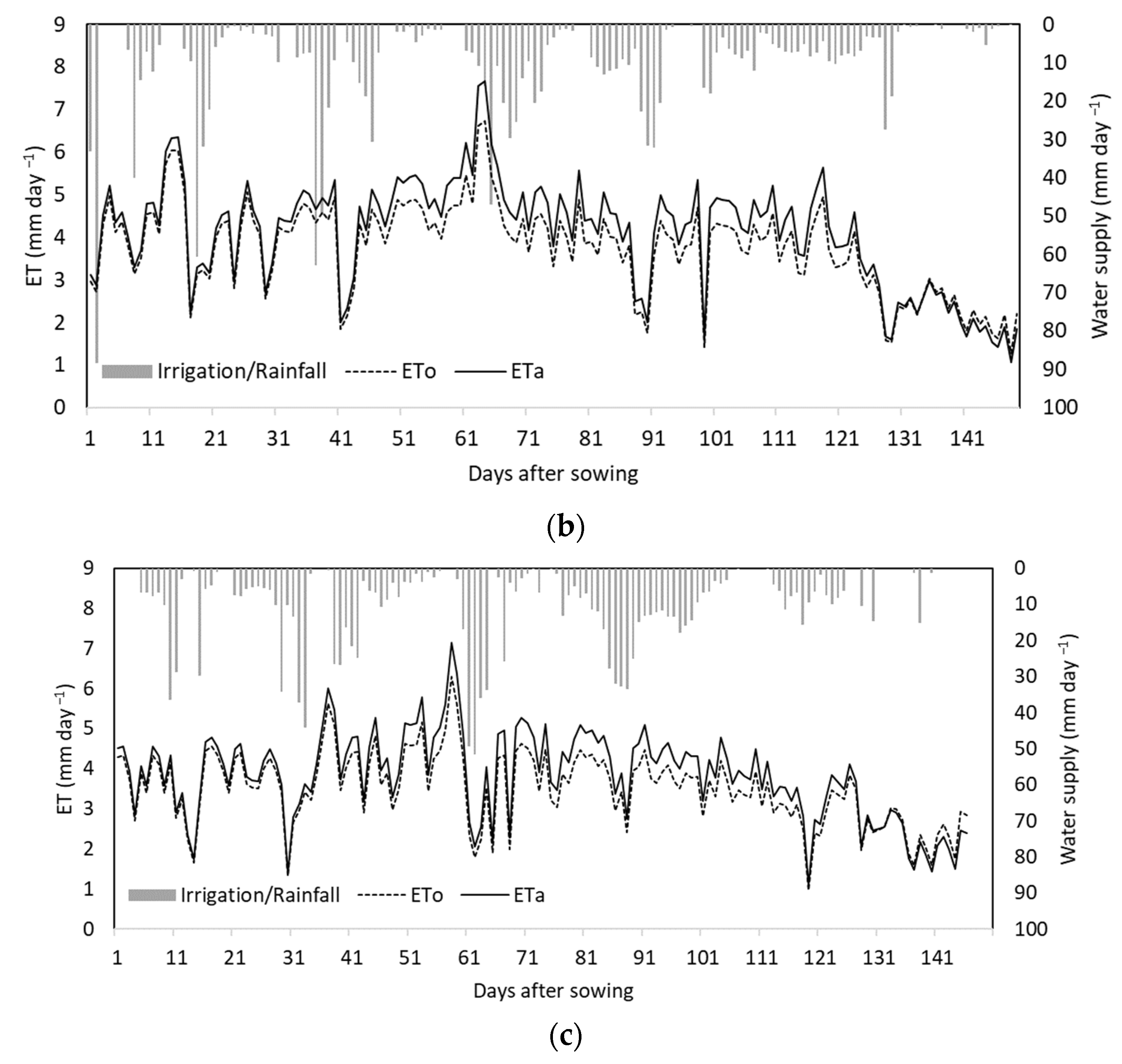
The results obtained in terms of the amount of irrigation, precipitation, evapotranspiration, and crop coefficients matched the growth stages of the crop. Regarding irrigation, which was only quantified in P1, the total values amounted to 1308 mm in 2019, 1263 mm in 2020, and 1206 mm in 2021, from the date of sowing to that of the harvest. Figure 3 shows the daily rice ETo and ETa data and the water input from the irrigation and precipitation for all the seasons. The irrigation applied in the initial stage (the first 30 days after sowing) was similar in 2019 and 2020 (370 and 360 mm, respectively). In 2021, the applied water was considerably lower (40% less) due to the abnormal precipitation in mid-June, which coincided in the initial phase [56]. The development stage (the next 30 days, which occurred between the second half of June and the second half of July) was more abundantly irrigated in 2019, with a total of 616 mm (more than double of that in 2020). In contrast, the middle stage (the next 60 days, until the second half of September) received half as much water in 2019 compared to 2020 and 2021, in response to the heat waves that occurred in both years during this time interval. In the final stage (which lasted the remaining time until harvest) the water application was drastically decreased and confined to the first 8–10 days, as mentioned in Section 2.1, as the grain was physiologically mature and harvest was being prepared.
The accumulated ETo during the rice growing seasons resulted 537 mm in 2019, 560 mm in 2020, and 511 mm in 2021. A higher average value (4.5 mm d−1) was denoted in the early phase of 2019 when compared to the same periods in 2020 and 2021 (4 mm d−1 and 3.6 mm d−1, respectively). In the development stage, the demand was higher in 2020 and 2021, which was related to the high relative humidity recorded in this period. In the middle stage, the average ETo tended to be similar to (2019) or lower than that in the previous phase (2020 and 2021). The drop in evaporative demand was specially noticed in the final phase, with values of around 2.1 mm d−1 (2019)–2.6 mm d−1 (2021).
Following the FAO56 methodology and the suggested values of Kc, as described in Section 2.2, the accumulated ETa during the rice growing seasons resulted 589 mm in 2019, 612 mm in 2020, and 557 mm in 2021. The difference between the total water applied and the ETa needs ranged between 719 mm (2019), 651 mm (2020), and 649 mm (2021); in practical terms, about half of the water applied to the rice crop was used for other components of irrigation water use, such as infiltration or percolation into the soil. The ETa values were higher than those obtained with ETo, because of the positive contribution given by Kc. The cultural practice of flooding in rice culture increases the challenge of quantifying the water requirements of this crop. The maximum tillering occurred about 34 days after sowing; this time interval corresponded to the initial stage, where the paddy fields were continuously covered with water, so the water losses via evaporation were high. The transpiration component of the rice plants was small during the early stages and was mainly due to the contribution from the leaf surface of the weeds, which established themselves rapidly.
3.3. NDVI
Figure 4 shows a comparison of the NDVIs obtained for the experimental plot (P1) and control plots (P2, P3, and P4) during the three campaigns. Each point represents the data of a single date from SPIDER, as explained in Section 2.4.
In 2019, the difference between the four plots was more noticeable for the first two phases. At the end of July (the development phase), the NDVI values ranged between 0.4 (P1 and P2) and 0.6 (P3 and P4). At the beginning of August, the four curves intersected, showing a homogeneous distribution. The NDVI peaked in mid-August (about 0.85). In 2020, the start was similar for the four plots. P3 showed a decrease in the NDVI at the end of June (initial phase). The curves for P1 and P3 remained superposed, reaching peaks at the end of August (about 0.8), while the same values were obtained about 15 days earlier for P2 and P4. The NDVI descent was homogeneous in the four plots. In 2021, P1, P2, and P3 remained practically overlapping throughout the cultural cycle. In turn, P4 showed a greater vegetative vigor until the end of June (the entire initial phase). The NDVI peak (between 0.78 and 0.85) was reached at the end of August for all the plots.
The results obtained show that the four plots followed similar NDVI value trends, especially from the development stage onwards. As their cultural management was the same, the differences may be due to a slight delay in the dates of sowing, treatments, and harvest, or even due to other issues concerning the plant health or soil characteristics. In the initial phase, there was some heterogeneity, which may be due to the rapid development of weeds in some plots. The effectiveness of the herbicide (applied about 35–40 days after sowing) translated into a lowering of the NDVI, which was quickly compensated for in the following phases. The use of four plots instead of only P1 increased the applicability of the methodology and allows us to reinforce and validate the results obtained. Focusing on P1, the NDVI evolution for the three rice growing seasons is plotted in Figure 5. For the 2020 campaign, the field measurements and values extracted from EEFlux were also superposed. Overall, the three NDVI sources show consistency for the 2020 trend.
The NDVI obtained from METRIC reflected a slight overestimation when compared to the SPIDER and field measurements. However, few Landsat 8 images were available (only five cloud-free images for this period), and the standard deviation, expressed in error bars, mitigated this difference. It should be also noted that the spatial resolution of the images considered in EEFlux (30 m) was lower than that provided by SPIDER (most images from Sentinel-2, with a resolution of 10 m).
The ground field measurements of the NDVIs in 2020 reproduced similar values to those of SPIDER. Nevertheless, from the end of July, all the registered values were lower. An explanation for this is that the plants closer to the berms of the field intended to develop less than the plants in the central area of the plot, having smaller foliar surfaces and consequently lower NDVIs, as a result of the passage of tractors and heavy vehicles. Despite the use of the extender, the reach of the vegetation further into the plot was limited. This method was important and useful for the calibration of the satellite images, but in the case of rice, where the fields were flooded most of the time, it only proved useful until the development phase, with limitations from the middle stage onwards, with the plants tapered and the plot covered.
The lowest NDVI values (less than 0.2), were identified in the initial phase of the rice crop cultivation and were due to the flooding of the plot. The highest NDVI values, of approximately 0.85 (2019), 0.80 (2020), and 0.83 (2021), were reached in mid-August, the end of August, and the beginning of September, respectively, corresponding to the middle phase, which also reflects the different sowing dates. Towards the end of the cultivation period, the NDVI values decreased until the plant reached full maturation and was harvested in the middle of October.
Figure 5 also shows, for the years of 2020 and 2021, the drop in the NDVI 40–45 days after the sowing date, as explained above.
3.4. Calibration of the RS-Assisted Kc-NDVI Relationship
Figure 4 and Figure 5 show that there was variability in the rice conditions among the different plots for a specific year and for the same plots in different years. This variability is clearly captured by the NDVI data from the satellite. However, the FAO56 methodology for deriving the ETa does not account for this, assigning the same crop coefficients for all the plots or surface conditions, with no distinction between the sowing dates. In this work, we introduce a technique based on the calibration of a Kc = Kc(NDVI) equation, adapted for our specific rice crop and local conditions, with the aim of further applying it to a temporal series of satellite images and reproducing the range of crop conditions under different management practices, leading to a variety of ETa values. This is the essence of the well-known RS-assisted FAO56 methodology, which has been successfully applied to a large variety of crops, but rarely seen for rice.
The NDVIs measured in the beginning of stage II were 0.43 (2019), 0.46 (2020), and 0.30 (2021); in stage III were 0.68 (2019), 0.66 (2020), and 0.57 (2021); and in stage IV were 0.74 (2019), 0.60 (2020), and 0.80 (2021). Upon relating the NDVI to the phenological phase of the rice, it was observed in the plot that: (i) the rice maximum tillering was at 34 DAS, (ii) panicle differentiation occurred at around 60 DAS, and (iii) flowering occurred at around 85 DAS. The average NDVIs measured in the maximum tillering were 0.43 (2019), 0.45 (2020), and 0.30 (2021); in the panicle differentiation were 0.67 (2019), 0.65 (2020), and 0.57 (2021); and at flowering, were 0.87 (2019), 0.77 (2020), and 0.74 (2021).
Using the data from 2019 as a basis, as this was a typical year in terms of meteorological circumstances, weed management, and crop yield, Kc was parametrized as a linear function of NDVI. Table 7 lists the coefficients for the linear regressions Kc-NDVI. These were only explored for stages II+III and IV because the high values of KCini in stage I were due to the presence of water (and its subsequent evaporation), while the NDVI values remain low in this case. A good correlation between the rice Kc and NDVIs in stages II+III was observed with an R2 of 0.82, RMSE of 0.000013, and BIAS value of 0.012. These results were even better for the regression corresponding to stage IV, with an R2 of 0.94, RMSE of 0.00002, and BIAS value of 0.020.
The Kc values suggested by the FAO56 for stages II+III and IV, in the three crop seasons, were replaced by those obtained from the Kc = Kc (NDVI) equations. The ETa was then recalculated for the full dataset to highlight the effect of considering this RS method in the variability of the results. The results are shown in Figure 6 for all the plots and show a good match among them for the three seasons, with some differences arising in P4 for 2020, from mid-phase III until the harvest.
3.5. Assessment of the ETa from RS-Assisted FAO56
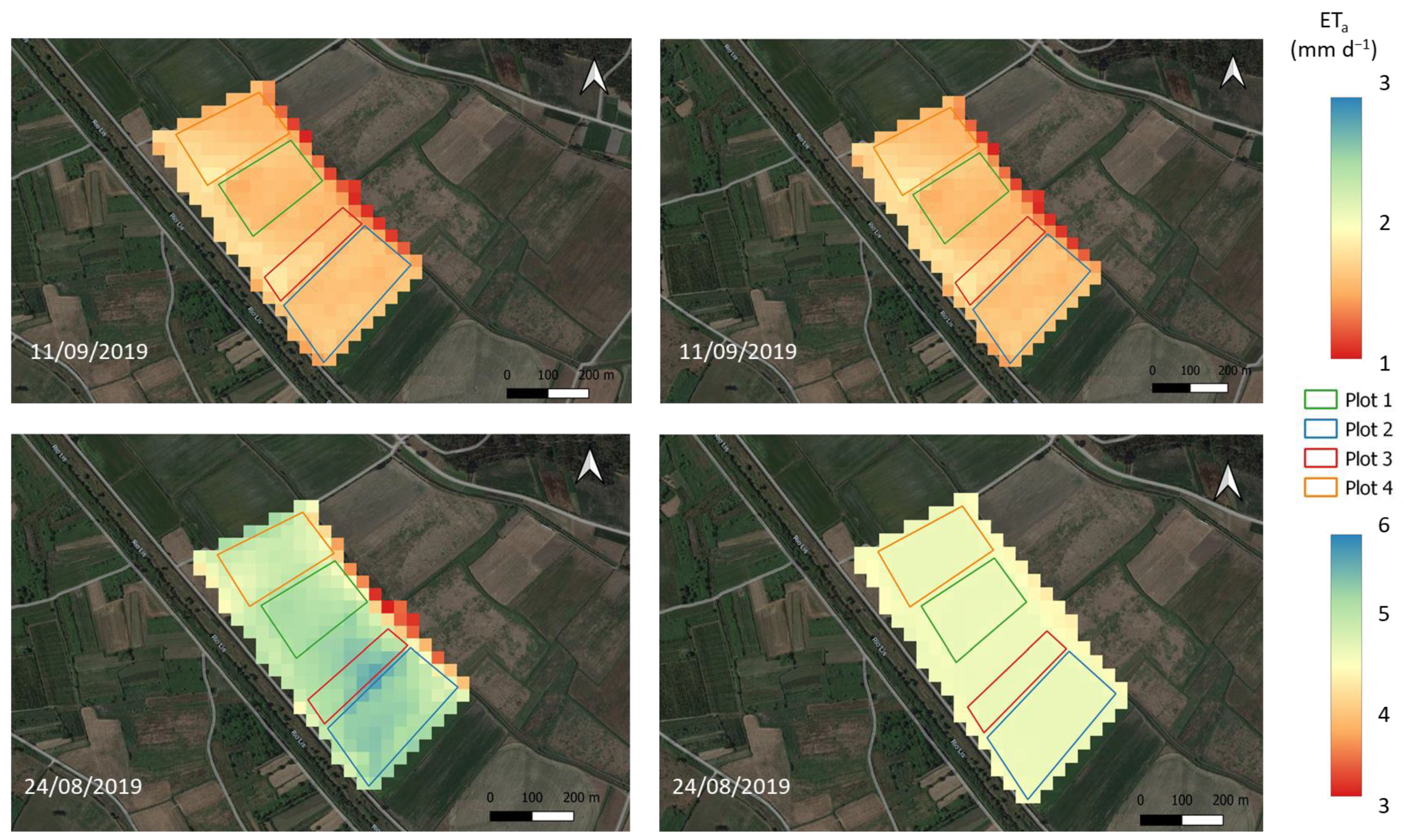
The independent ETa values provided by the surface energy balance model METRIC were used for the assessment of the established RS-assisted FAO56 technique. The maps in Figure 7 show two examples of the spatial distributions of ETa from both the METRIC and RS-assisted FAO56 approaches.
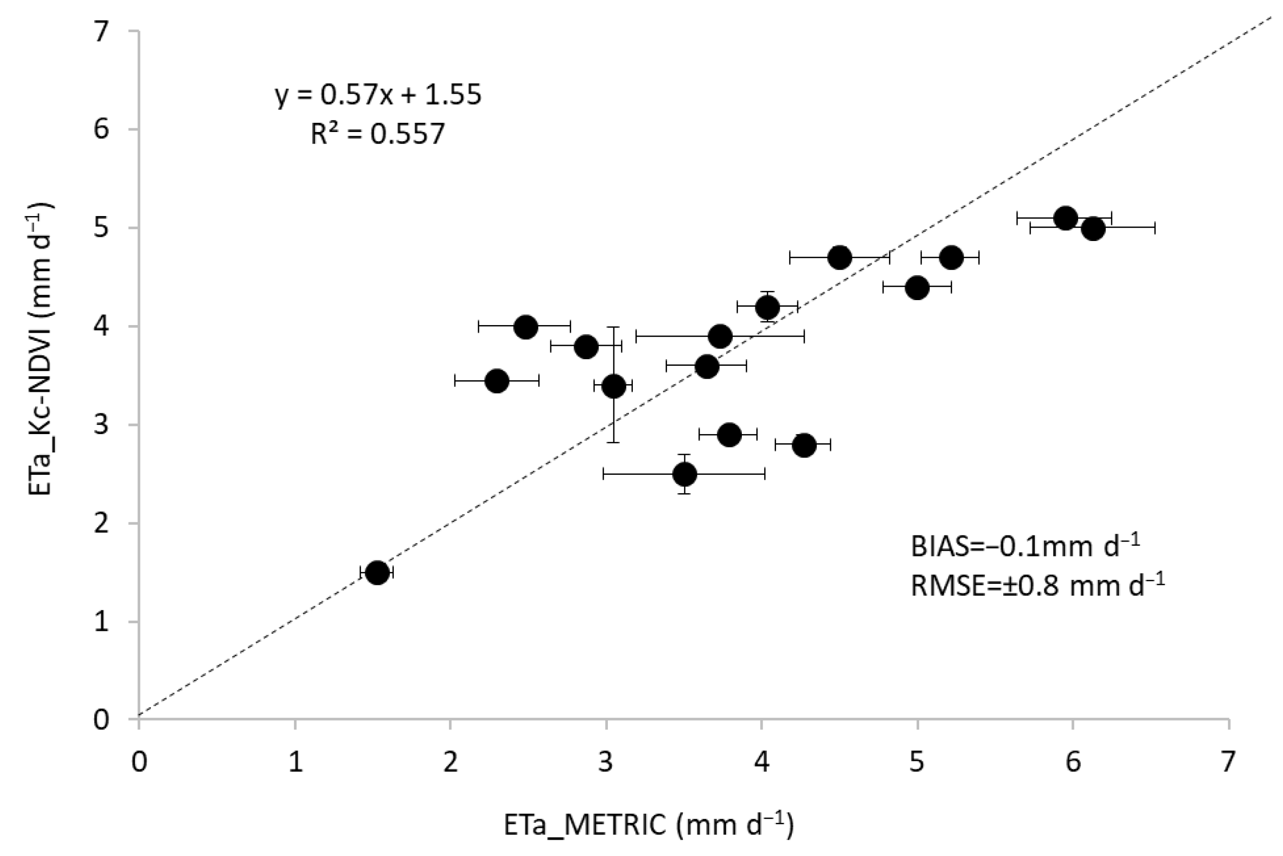
Figure 8 shows a comparison between the daily ETa values estimated from both methodologies, for the dates with availabilities of Landsat 8 images, for the three campaigns. The number of satellite images available was limited, due to the characteristic cloudiness of the LVID combined with the 16-day temporal resolution of Landsat 8. Note that the assessment was focused on stages II, III, and IV because of the reasons given in 3.4.
An average estimation error of ±0.8 mm d−1 with a negligible bias of −0.1 mm d−1 were obtained. The error bars in x translate the standard deviation of the ETa values obtained by METRIC.
3.6. Crop Yield and Irrigation Water Productivity
Table 8 shows a comparison between the rice ETa in P1, calculated by the FAO56 and obtained with the “RS-assisted” Kc. It also relates the yield results to the water consumption in P1 (the only plot where the amount of irrigation water was quantified) for the three experimental years. Once the samples of the mature plants were collected and analyzed, it was possible to relate both parameters to obtain the WP. The ETa, estimated from the FAO56, was very well matched with the results obtained using the RS approach for all the rice growing seasons. When the average ETa of the three years was compared, the results matched almost perfectly (586 mm and 585 mm from the FAO56 and RS approaches, respectively). The rice grain yield was higher in 2019 (7.5 t/ha), whereas in 2020 and 2021, it reached around 6 t/ha. The WP was slightly higher in 2019 (0.52 kg m−3) than in the following years (0.44–0.46 kg m−3). The season with the lowest WP corresponded to the highest ETa (2020). The WUE was higher in 2020 (0.45 kg m−3), while in 2019 and 2021, it remained at 0.41–0.42, respectively. The G was lower in 2021 (24 t/ha, when the ETa was also lower) than in the previous seasons (31.2 and 32 t/ha in 2019 and 2020, respectively). The rice straw was higher in 2019 (7.2 t/ha) and similar in 2020 and 2021 (4.1 and 4.2 t/ha).
4. Discussion
4.1. Evapotranspiration and Irrigation Water Applied
Rice is one of the largest cereal users of the world’s water resources. The evapotranspiration in flooded rice fields has been calculated in several studies, with results ranging from 4–7 mm d−1 [57,58]. In our study, the results of the ET ranged from 2.1 to 4.7 mm d−1. For the full crop season, the measured rice ETa was between 700 and 800 mm in Italy [59]. Sudhir-Yadav et al. [60] reported a rice ETa ranging between 749 and 811 mm under a semiarid climate in India, and Choudhury and Singh [61] found an ETa ranging from 781 to 899 mm in the semiarid climate of the Indo-Gangetic Plains in India. In California, the observed ETa ranged from 681 to 813 mm [62], and a significantly higher value of 1350 mm was reported in northern Greece [63].
The amount of irrigation water in rice, applied using the continuous flooding method, explains the concerns about water as a limited resource, both in terms of quality and quantity. The major identified problems are related to: (i) the water scarcity in several areas, exacerbated by drought events and the consequent deterioration of water quality; (ii) soil salinization and pollution in general, which have encouraged water policies leading to the rational use of this resource; and (iii) the effects of climate change [64]. In our study, the average irrigation water applied in the three seasons was 1259 mm, which is in line with the results obtained by other studies (e.g., 1208 mm [65] and 1291 mm [66]).
4.2. Crop Coefficient
In previous works, Allen et al. [11,51] reported rice Kc values adjusted to standard climate conditions (RHmin = 45% and u2 = 2 m s−1) of: KCini = 1.05, KCmid = 1.20, and KCend = 0.90–0.60. Several studies have been developed for the estimation of Kc in rice crops. In Zaragoza, Spain, for sprinkled irrigated rice, Moratiel and Martínez [13] indicated values of 0.92, 1.6, and 1.03 for KCini, KCmid, and KCend, respectively; in Sardinia, Italy, for those same stages and also using sprinkler irrigation, Spanu et al. [66] indicated coefficients of 0.9, 1.07, and 0.97. In this work, we accepted the Kc applicable to rice cultivation as proposed by FAO, but introduced a dependence on NDVI, which was provided by RS. The correlation between these two parameters allowed us to obtain an equation for the calculation of an “RS-assisted” Kc, applicable to stages II, III, and IV. The FAO56 suggests that the Kc remains the same during the initial phase, so we understand that the Kc—NDVI relationship could not be applied to this stage, because in the periods where the plots were flooded and the rice plants were not dense enough, the NDVI values became negative. This is the reason why some authors prefer to combine the NDVI with the Normalized Difference Water Index (NDWI), in order to depict the differences between rice paddies and non-rice paddy areas [67].
The FAO56 approach has been largely applied for crop water requirement estimations at a field plot spatial scale [11]. Both in the cases of dual Kc and single Kc, the FAO56 offers equations or tabulated values for Kc and Kcb at different crop stages. Following the recommendations of the authors themselves, in many countries, the Irrigation Advisory Services have adapted these tabulated values to crop varieties under specific climatic conditions. However, when large irrigated surface areas are monitored, the challenge of integrating crops, sowing dates, varieties, and local adaptations is higher. Nevertheless, the use of RS data has become a powerful link to applying the FAO56 approach, showing that RS products offer the capacity for monitoring crop growth over large and diverse areas [68]. As an example, in Spain, the software HidroMORE® has been tested over irrigation surface areas at different spatial and water resource scales, such as the aquifer [45] or Spanish mainland river basins [46], and at two water and agricultural management scales: the plot and the WUA scale [47]. Therefore, RS techniques have been sufficiently established for use, as required and requested by water managers [69], and the existence of global-free platforms that allow public access to satellite data products encourages their use.
4.3. Water Productivity and Crop Yield
Some researchers have reported a WP of rice at around 0.4 kg/m3 based on the total water input (irrigation plus rainfall) [70]. These data are in agreement with those obtained in the present study (an average value of 0.47 kg/m3 for the three seasons). Increasing this WP is a challenge that can be reached by: (i) improving the water use efficiency by reducing the applied water but maintaining the same yield, or (ii) improving the productivity (increasing the crop yield) with the same amount of consumed water. At the basin scale, with water being the first priority, the first approach is more desirable for establishing methods for reducing water consumption while maintaining food production, as suggested by Blatchford et al. [71]. If the goal aims to reduce the applied water, farmers should be encouraged to save this resource. However, farmers, especially smallholders with unfavorable financial conditions, typically have a tendency to prioritize yields rather than water consumption, regardless of the environmental consequences, as Pouladi et al. [72] perceived it. In the LVID, this issue is even more critical, since the rate of water use due to the WUA users is calculated according to the area of the plot and not the consumption, so cases of improper and irrational use are common. This situation is being mitigated by the rehabilitation works started in 2021, promoted by the National Irrigation Programme of Portugal [73], a governmental initiative that provides for the reconversion of irrigation systems. The original system is being replaced by pressure pipes, with meters being installed in the plots. In a recent study by Wei [74], a regional water-saving potential calculation method for paddy rice based on remote sensing (RWSP-RS) was proposed.
5. Conclusions
This study aimed to estimate the water requirements in rice paddy fields irrigated by the continuous flooding method, applying the FAO56 methodology to estimate the ETa, which was complemented by an RS approach using a temporal series of satellite NDVI images as its basis. Good correlations were found between the Kc proposed by the FAO and the NDVI evolution in the control rice fields, with an R2 ranging between 0.71 and 0.82 for stages II+III, and between 0.76 and 0.82 for stage IV. The results from the derived RS-assisted method were compared to the ETa values obtained from the surface energy balance model METRIC, showing an average estimation error of ±0.8 mm d−1 with a negligible bias. The findings in this work are promising and show the potential of the RS-assisted method for monitoring ETa and water productivity, capturing the local and seasonal variability in rice growing, and predicting rice yield, being a useful and free tool available to farmers. To our knowledge, this is the first report of a study in which the ETa provided by the METRIC platform is compared with the ETa calculated by the FAO56 methodology. The reach of this study also fulfills the requirements from basin-scale water managers, and so can be integrated into large-scale irrigation networks to improve the water management of continuous flooded rice production.
Some final considerations about this study may guide further work, namely: (1) the characteristic cloudiness in the study site limited the acquisition of satellite images. Additionally, depending on the field size, the Landsat spatial resolution might not be appropriate. Further studies should integrate higher resolution platforms such as Planet scope; (2) the NDVI saturates for dense full vegetated covers. Further studies may explore the use of additional VIs; and (3) it will be interesting to expand the assessment of the calibrated Kc = Kc(NDVI) equation to other rice production areas with a similar agronomic management.
Author Contributions
J.M.S. and J.M.G. conceptualize and design the study; S.F. and J.M.G. performed the field observations; S.F., J.M.S. and J.M.G. analyzed and validated the data; S.F. wrote the paper with contributions of the other authors. All authors have read and agreed to the published version of the manuscript.
Funding
This research and APC was funded by (i) Project Grupo Operacional para a Gestão da Água no Vale do Lis, PDR2020–1.0.1-FEADER-030911, funded by Program PDR2020, co-funded by FEDER, Innovation Measure, Portugal, (ii) Project “MEDWATERICE”, PRIMA/0005/2018, funded by the Portuguese Science and Technology Foundation (FCT) and (iii) PhD research grant funded by Portuguese Foundation for Science and Technology, ref. 2020.07088.BD.
Data Availability Statement
The data presented in this study are available on request from the corresponding author.
Conflicts of Interest
The authors declare no conflict of interest.
References
- Awika, J.M. Major Cereal Grains Production and Use around the World. In Advances in Cereal Science: Implications to Food Processing and Health Promotion; ACS Symposium Series 1089; American Chemical Society: Washington, DC, USA, 2001; Volume 1089, pp. 1–13. [Google Scholar] [CrossRef]
- FAOSTAT. Available online: http://www.fao.org/faostat/en/#data/QC/visualize (accessed on 15 December 2022).
- INE Database. Agricultural Forecasts. INE: Lisbon, Portugal. Available online: https://www.ine.pt/xportal/xmain?xpid=INE&xpgid=ine_destaques&DESTAQUESdest_boui=473554484&DESTAQUESmodo=2&xlang=pt (accessed on 17 February 2022).
- Kaspary, T.E.; Roma-Burgos, N.; Merotto, A., Jr. Snorkeling Strategy: Tolerance to Flooding in Rice and Potential Application for Weed Management. Genes 2020, 11, 975. [Google Scholar] [CrossRef] [PubMed]
- Chen, Y.; Zhang, G.; Xu, Y.J.; Huang, Z. Influence of Irrigation Water Discharge Frequency on Soil Salt Removal and Rice Yield in a Semi-Arid and Saline-Sodic Area. Water 2013, 5, 578–592. [Google Scholar] [CrossRef]
- De Bauw, P.; Vandamme, E.; Lupembe, A.; Mwakasege, L.; Senthilkumar, K.; Merckx, R. Architectural Root Responses of Rice to Reduced Water Availability Can Overcome Phosphorus Stress. Agronomy 2019, 9, 11. [Google Scholar] [CrossRef]
- Gómez de Barreda, D.; Pardo, G.; Osca, J.M.; Catala-Forner, M.; Consola, S.; Garnica, I.; López-Martínez, N.; Palmerín, J.A.; Osuna, M.D. An Overview of Rice Cultivation in Spain and the Management of Herbicide-Resistant Weeds. Agronomy 2021, 11, 1095. [Google Scholar] [CrossRef]
- Zampieri, M.; Ceglar, A.; Manfron, G.; Toreti, A.; Duveiller, G.; Romani, M.; Rocca, C.; Scoccimarro, E.; Podrascanin, Z.; Djurdjevic, V. Adaptation and sustainability of water management for rice agriculture in temperate regions: The Italian case-study. Land Degrad Dev. 2019, 30, 2033–2047. [Google Scholar] [CrossRef]
- Zampieri, E.; Pesenti, M.; Nocito, F.F.; Sacchi, G.A.; Valè, G. Rice Responses to Water Limiting Conditions: Improving Stress Management by Exploiting Genetics and Physiological Processes. Agriculture 2023, 13, 464. [Google Scholar] [CrossRef]
- Ringler, C.; Zhu, T. Water Resources and Food Security. Agronomy 2015, 107, 1533–1538. [Google Scholar] [CrossRef]
- Allen, R.G.; Raes, D.; Smith, M. Crop Evapotranspiration: Guidelines for Computing Crop Requirements; Irrigation and Drainage Paper No. 56; FAO: Rome, Italy, 1998. [Google Scholar]
- Yang, Y.; Feng, Z.; Huang, H.Q.; Lin, Y. Climate-induced changes in crop water balance during 1960–2001 in Northwest China. Agric. Ecosyst. Environ. 2008, 127, 107–118. [Google Scholar] [CrossRef]
- Moratiel, R.; Martínez-Cob, A. Evapotranspiration and crop coefficients of rice (Oryza sativa L.) under sprinkler irrigation in a semiarid climate determined by the surface renewal method. Irrig. Sci. 2011, 31, 411–422. [Google Scholar] [CrossRef]
- Yan, H.; Zhang, C.; Oue, H.; Peng, G.; Darko, R. Determination of crop and soil evaporation coefficients for estimating evapotranspiration in a paddy field. Int. J. Agric. Biol. Eng. 2017, 10, 130–139. [Google Scholar] [CrossRef]
- Liu, B.; Cui, Y.; Shi, Y. Comparison of evapotranspiration measurements between eddy covariance and lysimeters in paddy fields under alternate wetting and drying irrigation. Paddy Water Environ. 2019, 17, 725–739. [Google Scholar] [CrossRef]
- Moran, M.S.; Jackson, R.D. Assessing the Spatial Distribution of Evapotranspiration Using Remotely Sensed Inputs. J. Environ. Qual. 1991, 20, 725–737. [Google Scholar] [CrossRef]
- Allen, R.G.; Pereira, L.S.; Howell, T.A.; Jensen, M.E. Evapotranspiration Information Reporting: I. Factors Governing Measurement Accuracy. Agric. Water Manag. 2011, 23, 899–920. [Google Scholar] [CrossRef]
- Liou, Y.A.; Chuang, Y.C.; Lee, T. Estimate of evapotranspiration over rice fields using high resolution DMSV imagery data. In Proceedings of the Cross-Strait Symposium on the Remote Sensing and Agricultural Biotechnology, Chung-li, Taiwan, 22–25 February 2002. [Google Scholar]
- Fawzy, H.E.; Sakr, A.; El-Enany, M.; Moghazy, H.M. Spatiotemporal assessment of actual evapotranspiration using satellite remote sensing technique in the Nile Delta, Egypt. Alex. Eng. J. 2021, 60, 1421–1432. [Google Scholar] [CrossRef]
- Quille Mamani, J.; Ramos-Fernández, L.; Ontiveros-Capurata, R.E. Estimación de la evapotranspiración del cultivo de arroz en Perú mediante el algoritmo METRIC e imágenes VANT/Estimation of rice crop evapotranspiration in Perú based on the METRIC algorithm and UAV images. Rev. Teledetec. 2021, 58, 23–38. [Google Scholar] [CrossRef]
- Jiang, C.; Ryu, Y. Multi-scale evaluation of global gross primary productivity and evapotranspiration products derived from Breathing Earth System Simulator (BESS). Remote Sens. Environ. 2016, 186, 528–547. [Google Scholar] [CrossRef]
- Gan, G.; Zhao, X.; Fan, X.; Xie, H.; Jin, W.; Zhou, H.; Cui, Y.; Liu, Y. Estimating the Gross Primary Production and Evapotranspiration of Rice Paddy Fields in the Sub-Tropical Region of China Using a Remotely-Sensed Based Water-Carbon Coupled Model. Remote Sens. 2021, 13, 3470. [Google Scholar] [CrossRef]
- Xue, W.; Jeong, S.; Ko, J.; Yeom, J.-M. Contribution of Biophysical Factors to Regional Variations of Evapotranspiration and Seasonal Cooling Effects in Paddy Rice in South Korea. Remote Sens. 2021, 13, 3992. [Google Scholar] [CrossRef]
- Pokorny, J. Evapotranspiration. In Encyclopedia of Ecology, 2nd ed.; Elsevier: Amsterdam, The Netherlands, 2019; pp. 292–303. [Google Scholar] [CrossRef]
- Odhiambo, L.O.; Irmak, S. Evaluation of the impact of surface residue cover on single and dual crop coefficient for estimating soybean actual evapotranspiration. Agric. Water Manag. 2012, 104, 221–234. [Google Scholar] [CrossRef]
- Pereira, L.S.; Allen, R.G.; Smith, M.; Raes, D. Crop evapotranspiration estimation with FAO56: Past and future. Agric. Water Manag. 2015, 147, 4–20. [Google Scholar] [CrossRef]
- Xing, N.; Huang, W.; Xie, Q.; Shi, Y.; Ye, H.; Dong, Y.; Wu, M.; Sun, G.; Jiao, Q. A Transformed Triangular Vegetation Index for Estimating Winter Wheat Leaf Area Index. Remote Sens. 2020, 12, 16. [Google Scholar] [CrossRef]
- Guan, S.; Fukami, K.; Matsunaka, H.; Okami, M.; Tanaka, R.; Nakano, H.; Sakai, T.; Nakano, K.; Ohdan, H.; Takahashi, K. Assessing Correlation of High-Resolution NDVI with Fertilizer Application Level and Yield of Rice and Wheat Crops Using Small UAVs. Remote Sens. 2019, 11, 112. [Google Scholar] [CrossRef]
- González-Betancourt, M.; Mayorga-Ruíz, Z.L. Normalized difference vegetation index for rice management in El Espinal, Colombia. DYNA 2018, 85, 47–56. [Google Scholar] [CrossRef]
- Xue, J.; Su, B. Significant remote sensing vegetation indices: A review of developments and applications. J. Sens. 2017, 2017, 1353691. [Google Scholar] [CrossRef]
- Imran, H.A.; Gianelle, D.; Rocchini, D.; Dalponte, M.; Martín, M.P.; Sakowska, K.; Wohlfahrt, G.; Vescovo, L. VIS-NIR, Red-Edge and NIR-Shoulder Based Normalized Vegetation Indices Response to Co-Varying Leaf and Canopy Structural Traits in Heterogeneous Grasslands. Remote Sens. 2020, 12, 2254. [Google Scholar] [CrossRef]
- Zheng, H.; Cheng, T.; Li, D.; Zhou, X.; Yao, X.; Tian, Y.; Cao, W.; Zhu, Y. Evaluation of RGB, Color-Infrared and Multispectral Images Acquired from Unmanned Aerial Systems for the Estimation of Nitrogen Accumulation in Rice. Remote Sens. 2018, 10, 824. [Google Scholar] [CrossRef]
- Rabatel, G.; Gorretta, N.; Labbé, S. Getting simultaneous red and near-infrared band data from a single digital camera for plant monitoring applications: Theoretical and practical study. Biosyst. Eng. 2014, 117, 2–14. [Google Scholar] [CrossRef]
- Mirzaee, S.; Mirzakhani Nafchi, A. Monitoring Spatiotemporal Vegetation Response to Drought Using Remote Sensing Data. Sensors 2023, 23, 2134. [Google Scholar] [CrossRef] [PubMed]
- Panek, E.; Gozdowski, D. Analysis of relationship between cereal yield and NDVI for selected regions of Central Europe based on MODIS satellite data. Remote Sens. Appl. Soc. Environ. 2020, 17, 100286. [Google Scholar] [CrossRef]
- Park, J.; Baik, J.; Choi, M. Satellite-based crop coefficient and evapotranspiration using surface soil moisture and vegetation indices in Northeast Asia. CATENA 2017, 156, 305–314. [Google Scholar] [CrossRef]
- Taherparvar, M.; Pirmoradian, N. Estimation of Rice Evapotranspiration Using Reflective Images of Landsat Satellite in Sefidrood Irrigation and Drainage Network. Rice Sci. 2018, 25, 111–116. [Google Scholar] [CrossRef]
- French, A.N.; Hunsaker, D.J.; Sanchez, C.A.; Saber, M.; Gonzalez, J.R.; Anderson, R. Satellite-based NDVI crop coefficients and evapotranspiration with eddy covariance validation for multiple durum wheat fields in the US Southwest. Agric. Water Manag. 2020, 239, 106266. [Google Scholar] [CrossRef]
- Gontia, N.K.; Tiwari, K.N. Estimation of Crop Coefficient and Evapotranspiration of Wheat (Triticum aestivum) in an Irrigation Command Using Remote Sensing and GIS. Water Resour Manag. 2010, 24, 1399–1414. [Google Scholar] [CrossRef]
- Lei, H.; Yang, D. Combining the crop coefficient of winter wheat and summer maize with a remotely sensed vegetation index for estimating evapotranspiration in the North China plain. J. Hydrol. Eng. 2014, 19, 243–251. [Google Scholar] [CrossRef]
- Lima, J. Water requirement and crop coefficients of sorghum in Apodi Plateau. Rev. Bras. Eng. Agríc. Ambient. 2021, 25, 684–688. [Google Scholar] [CrossRef]
- Campos, I.; Neale, C.M.U.; Calera, A.; Balbontín, C.; González-Piqueras, J. Assessing satellite-based basal crop coefficients for irrigated grapes (Vitis vinifera L.). Agric. Water Manag. 2010, 98, 45–54. [Google Scholar] [CrossRef]
- Moreno, R.; Arias, E.; Sánchez, J.L.; Cazorla, D.; Garrido, J.; Gonzalez-Piqueras, J. HidroMORE 2: An optimized and parallel version of HidroMORE. In Proceedings of the 2017 8th International Conference on Information and Communication Systems (ICICS), Irbid, Jordan, 4–6 April 2017; pp. 1–6. [Google Scholar]
- Sánchez, N.; Martínez-Fernández, J.; Calera, A.; Torres, E.; Pérez-Gutiérrez, C. Combining remote sensing and in situ soil moisture data for the application and validation of a distributed water balance model (HIDROMORE). Agric. Water Manag. 2010, 98, 69–78. [Google Scholar] [CrossRef]
- Garrido-Rubio, J.; Sanz, D.; González-Piqueras, J. Application of a remote sensing-based soil water balance for the accounting of groundwater abstractions in large irrigation areas. Irrig. Sci. 2019, 37, 709–724. [Google Scholar] [CrossRef]
- Garrido-Rubio, J.; Calera, A.; Arellano, I.; Belmonte, M.; Fraile, L.; Ortega, T.; Bravo, R.; González-Piqueras, J. Evaluation of Remote Sensing-Based Irrigation Water Accounting at River Basin District Management Scale. Remote Sens. 2020, 12, 3187. [Google Scholar] [CrossRef]
- Garrido-Rubio, J.; González-Piqueras, J.; Campos, I.; Osann, A.; González-Gómez, L.; Calera, A. Remote sensing–based soil water balance for irrigation water accounting at plot and water user association management scale. Agric. Water Manag. 2020, 238, 106236. [Google Scholar] [CrossRef]
- Ferreira, S.; Oliveira, F.; Gomes da Silva, F.; Teixeira, M.; Gonçalves, M.; Eugénio, R.; Damásio, H.; Gonçalves, J.M. Assessment of Factors Constraining Organic Farming Expansion in Lis Valley, Portugal. AgriEngineering 2020, 2, 111–127. [Google Scholar] [CrossRef]
- Gonçalves, J.M.; Ferreira, S.; Nunes, M.; Eugénio, R.; Amador, P.; Filipe, O.; Duarte, I.M.; Teixeira, M.; Vasconcelos, T.; Oliveira, F.; et al. Developing Irrigation Management at District Scale Based on Water Monitoring: Study on Lis Valley, Portugal. AgriEngineering 2020, 2, 78–95. [Google Scholar] [CrossRef]
- Gonçalves, J.M.; Nunes, M.; Ferreira, S.; Jordão, A.; Paixão, J.; Eugénio, R.; Russo, A.; Damásio, H.; Duarte, I.M.; Bahcevandziev, K. Alternate Wetting and Drying in the Center of Portugal: Effects on Water and Rice Productivity and Contribution to Development. Sensors 2022, 22, 3632. [Google Scholar] [CrossRef] [PubMed]
- Doorenbos, J.; Pruitt, W.O. Crop Water Requirements; Irrigation and Drainage Paper No. 24; FAO: Rome, Italy, 1997. [Google Scholar]
- Allen, R.G.; Tasumi, M.; Morse, A.; Trezza, R.; Wright, J.L. Satellite-Based Energy Balance for Mapping Evapotranspiration with Internalized Calibration (METRIC)—Applications. J. Irrig. Drain. Eng. 2007, 133, 395–406. [Google Scholar] [CrossRef]
- Laounia, N.; Abderrahmane, H.; Abdelkader, K.; Zahira, S.; Mansour, Z. Evapotranspiration and Surface Energy Fluxes Estimation Using the Landsat-7 Enhanced Thematic Mapper Plus Image over a Semiarid Agrosystem in the North-West of Algeria. Rev. Bras. Meteorol. 2017, 32, 691–702. [Google Scholar] [CrossRef]
- IPMA. Resumo Climatológico, Ano 2019. IPMA, Lisbon, Portugal (in Portuguese). Available online: https://www.ipma.pt/pt/publicacoes/boletins.jsp?cmbDep=cli&cmbTema=pcl&cmbAno=2021&idDep=cli&idTema=pcl&curAno=20 (accessed on 15 May 2022).
- IPMA. Resumo Climatológico, Ano 2020. IPMA, Lisbon, Portugal (in Portuguese). Available online: https://www.ipma.pt/pt/publicacoes/boletins.jsp?cmbDep=cli&cmbTema=pcl&cmbAno=2021&idDep=cli&idTema=pcl&curAno=20 (accessed on 15 May 2022).
- IPMA. Resumo Climatológico, Ano 2021. IPMA, Lisbon, Portugal (in Portuguese). Available online: https://www.ipma.pt/pt/publicacoes/boletins.jsp?cmbDep=cli&cmbTema=pcl&cmbAno=2021&idDep=cli&idTema=pcl&curAno=20 (accessed on 15 May 2022).
- Alberto, M.C.R.; Wassmann, R.; Hirano, T.; Miyata, A.; Hatano, R.; Kumar, A.; Padre, A.; Amante, M. Comparisons of energy balance and evapotranspiration between flooded and aerobic rice fields in the Philippines. Agric. Water Manag. 2011, 98, 1417–1430. [Google Scholar] [CrossRef]
- Lage, M.; Bamouh, A.; Karrou, M.; El Mourid, M. Estimation of rice evapotranspiration using a microlysimeter technique and comparison with FAO Penman-Monteith and Pan evaporation methods under Moroccan conditions. Agronomie 2003, 23, 625–631. [Google Scholar] [CrossRef]
- Djaman, K.; Rudnick, D.R.; Moukoumbi, Y.D.; Sow, A.; Irmak, S. Actual evapotranspiration and crop coefficients of irrigated lowland rice (Oryza sativa L.) under semiarid climate. Ital. J. Agron. 2019, 14, 19–25. [Google Scholar] [CrossRef]
- Sudhir-Yadav; Humphreys, E.; Kukal, S.S.; Gill, G.; Rangarajan, R. Effect of water management on dry seeded and puddled transplanted rice: Part 2: Water balance and water productivity. Field Crops Res. 2011, 120, 123–132. [Google Scholar] [CrossRef]
- Singh, N.; Choudhury, D.R.; Tiwari, G.; Singh, A.K.; Kumar, S.; Srinivasan, K.; Tyagi, R.K.; Sharma, A.D.; Singh, N.K.; Singh, R. Genetic diversity trend in Indian rice varieties: An analysis using SSR markers. BMC Genet 2016, 17, 127. [Google Scholar] [CrossRef]
- Montazar, A.; Rejmanek, H.; Tindula, G.; Little, C.; Shapland, T.; Anderson, F.; Inglese, G.; Mutters, R.; Linquist, B.; Greer, C.A.; et al. Crop Coefficient Curve for Paddy Rice from Residual Energy Balance Calculations. J. Irrig. Drain. Eng. 2017, 143. [Google Scholar] [CrossRef]
- Lekakis, E.; Aschonitis, V.; Pavlatou-Ve, A.; Papadopoulos, A.; Antonopoulos, V. Analysis of temporal variation of soil salinity during the growing season in a Flooded Rice Field of Thessaloniki Plain-Greece. Agronomy 2015, 5, 35–54. [Google Scholar] [CrossRef]
- Monaco, F.; Guido, S. How water amounts and management options drive Irrigation Water Productivity of rice. A multivariate analysis based on field experiment data. Agric. Water Manag. 2018, 195, 47–57. [Google Scholar] [CrossRef]
- Gonçalves, J.M.; Nunes, M.; Jordão, A.; Ferreira, S.; Eugénio, R.; Bigeriego, J.; Duarte, I.; Amador, P.; Filipe, O.; Damásio, H.; et al. The Challenges of Water Saving in Rice Irrigation: Field Assessment of Alternate Wetting and Drying Flooding and Drip Irrigation Techniques in the Lis Valley, Portugal. In Proceedings of the 1st International Conference on Water Energy Food and Sustainability (ICoWEFS 2021), Leiria, Portugal; Springer: Cham, Switzerland, 2021. [Google Scholar] [CrossRef]
- Spanu, A.; Murtas, A.; Ballone, F. Water Use and Crop Coefficients in Sprinkler Irrigated Rice. Ital. J. Agron. 2009, 4, 47–58. [Google Scholar] [CrossRef]
- Gao, B.-C. NDWI-A Normalized Difference Water index for Remote Sensing of Vegetation Liquid Water from Space. Remote Sens. Environ. 1996, 58, 257–266. [Google Scholar] [CrossRef]
- Tasumi, M.; Allen, R.G. Satellite-based ET mapping to assess variation in ET with timing of crop development. Agric. Water Manag. 2006, 88, 54–62. [Google Scholar] [CrossRef]
- Calera, A.; Campos, I.; Osann, A.; D’Urso, G.; Menenti, M. Remote sensing for crop water management: From ET modelling to services for the end users. Sensors 2017, 17, 1104. [Google Scholar] [CrossRef]
- Tuong, T.P.; Bam, B.; Mortimer, M. More rice, less water—Integrated approaches for increasing water productivity in irrigated rice-based systems in Asia. J. Plant Prod. Sci. 2005, 8, 231–241. [Google Scholar] [CrossRef]
- Blatchford, M.L.; Karimi, P.; Bastiaanssen, W.G.M.; Nouri, H. From Global Goals to Local Gains—A Framework for Crop Water Productivity. ISPRS Int. J. Geo.-Inf. 2018, 7, 414. [Google Scholar] [CrossRef]
- Pouladi, P.; Badiezadeh, S.; Pouladi, M.; Yousefi, P.; Farahmand, H.; Kalantari, Z.; Yu, D.J.; Sivapalan, M. Interconnected governance and social barriers impeding the restoration process of Lake Urmia. J. Hydrol. 2021, 598, 126489. [Google Scholar] [CrossRef]
- Diário da República. Presidency of the Council of Ministers No.77/2018, Republic Diary, 1st Series—No. 197—12 October 2018. Available online: https://files.dre.pt/1s/2018/10/19700/0494804957.pdf (accessed on 15 January 2023).
- Wei, J.; Cui, Y.; Zhou, S.; Luo, Y. Regional water-saving potential calculation method for paddy rice based on remote sensing. Agric. Water Manag. 2022, 267, 107610. [Google Scholar] [CrossRef]
Figure 1.
Areas cultivated with rice in LVID (map updated in June 2022). Red line represents the delimitation of LVID; blue line represents Lis river; and rose and yellow colors represent the plots cultivated with rice by two farmers: José Manuel (JM) and Nuno Guilherme (NG), respectively. (Source: LVID Water Users’ Association, 2022). In the lower left corner is shown the configuration of P1 (green line), P2 (blue line), P3 (red line), and P4 (orange line) (source: Google Earth, https://earth.google.com, accessed on 15 January 2023).

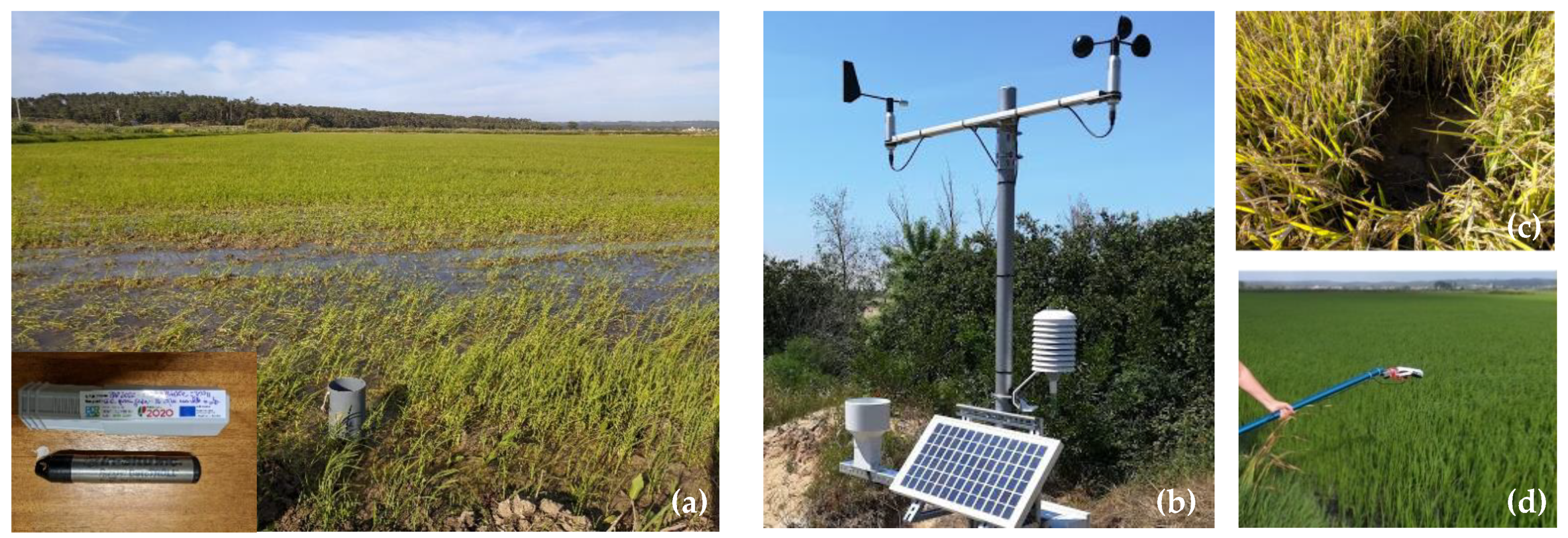
Figure 2.
Tube installed in the experimental plot (P1); in the lower left corner, Rugged Troll 100 limnigraph (a), automatic agrometeorological station (b), view of an area where samples were taken (c), and manual measures of NDVI with GreenSeeker Handheld Crop Sensor, with an extensor coupled (d).
Figure 2.
Tube installed in the experimental plot (P1); in the lower left corner, Rugged Troll 100 limnigraph (a), automatic agrometeorological station (b), view of an area where samples were taken (c), and manual measures of NDVI with GreenSeeker Handheld Crop Sensor, with an extensor coupled (d).

Figure 3.
Daily reference evapotranspiration (ETo) and daily actual evapotranspiration (ETa) values calculated during 2019 (a), 2020 (b), and 2021 (c) rice growing seasons in the study site. Irrigation and precipitation in P1 are depicted with vertical bars.
Figure 3.
Daily reference evapotranspiration (ETo) and daily actual evapotranspiration (ETa) values calculated during 2019 (a), 2020 (b), and 2021 (c) rice growing seasons in the study site. Irrigation and precipitation in P1 are depicted with vertical bars.


Figure 4.
NDVI evolution in P1 (experimental plot), and P2, P3, and P4 (control plots), from the constellation Sentinel 2+Landsat for seasons 2019 (a), 2020 (b), and 2021 (c).
Figure 4.
NDVI evolution in P1 (experimental plot), and P2, P3, and P4 (control plots), from the constellation Sentinel 2+Landsat for seasons 2019 (a), 2020 (b), and 2021 (c).

Figure 5.
NDVI extracted from SPIDER (graph lines, for 2019, 2020, and 2021), ground field measurements (2020), and METRIC EEFlux (2020). Error bars represent the standard deviation in the field measurements or the 3 × 3 pixel averages from METRIC, in each case.
Figure 5.
NDVI extracted from SPIDER (graph lines, for 2019, 2020, and 2021), ground field measurements (2020), and METRIC EEFlux (2020). Error bars represent the standard deviation in the field measurements or the 3 × 3 pixel averages from METRIC, in each case.

Figure 6.
ETa from RS-assisted FAO56 evolution in P1 (experimental plot), and P2, P3, and P4 (control plots), for stages II-IV, for seasons 2019 (a), 2020 (b), and 2021 (c).
Figure 6.
ETa from RS-assisted FAO56 evolution in P1 (experimental plot), and P2, P3, and P4 (control plots), for stages II-IV, for seasons 2019 (a), 2020 (b), and 2021 (c).

Figure 7.
Examples of ETa maps obtained from METRIC (left) and RS-assisted FAO56 approach (right) for two different dates: 11 October 2019 (upper) and 24 August 2019 (lower). The rice plots are delimited with green (P1), blue (P2), red (P3), and orange (P4) lines.
Figure 7.
Examples of ETa maps obtained from METRIC (left) and RS-assisted FAO56 approach (right) for two different dates: 11 October 2019 (upper) and 24 August 2019 (lower). The rice plots are delimited with green (P1), blue (P2), red (P3), and orange (P4) lines.

Figure 8.
Linear regression between mean values of ETa provided by METRIC and ETa calculated from the Kc = Kc(NDVI) relationship derived. Dotted line represents the 1:1 agreement. Error bars indicate the spatial variability, representing the standard deviation in ETa values from METRIC in the x axis, and in the ETa resulting from the Kc = Kc(NDVI) approach in the y axis.


Table 1.
Sensors characteristics applied for the hydraulic monitoring system.
| Parameter | Brand and Model |
|---|---|
| Water level | In-Situ Inc., model Rugged TROLL 100, Fort Collins, CO, USA |
| Atmospheric pressure | In-Situ Inc., model Rugged Baro TROLL, Fort Collins, CO, USA |
| Water flow velocity | VALEPORT, EM flow meter model 801 flat, Decon, UK |
Adapted from [43].
Table 2.
Sensors characteristics used in the automated agrometeorological station.
| Parameter | Brand and Model |
|---|---|
| Pluviometer | Pronamic ApS, diam. 16 cm, Ringkøbing, Denmark |
| Data logger | Campbell Scientific, Inc. CR300, Logan, UT, USA |
| Air temperature and humidity | Campbell Scientific, Inc. EE181, Logan, UT, USA |
| Solar radiation | Campbell Scientific, Inc. CS301, Logan, UT, USA |
| Wind speed | Lambrecht meteo GmbH, ORA, Göttingen, Germany |
| Remote communication of weather station | Cinterion, BGS2 Terminal RS232, Praha, Czech Republic |
Adapted from [50].
Table 3.
Crop development and irrigation practices and corresponding dates, with reference to 2019 rice growing season in LVID.
Table 3.
Crop development and irrigation practices and corresponding dates, with reference to 2019 rice growing season in LVID.
| Crop Development and Irrigation Practices | Days after Sowing (DAS) |
|---|---|
| Initial soil flooding | −1 |
| Wet sowing | 0 |
| Start tillering | 34 |
| Panicle differentiation | 60 |
| Flowering | 85 |
| Last irrigation event | 140 |
| Harvest | 152 |
Adapted from [50].
Table 4.
Landsat 8 images acquisition date, available for this work, and the corresponding season crop growth stage.
Table 4.
Landsat 8 images acquisition date, available for this work, and the corresponding season crop growth stage.
| Image Acquisition Date | Season Crop Growth Stages |
|---|---|
| 2019 | |
| 21 June | I |
| 07 July | II |
| 23 July | III |
| 24 August | III |
| 9 September | III |
| 11 October | IV |
| 2020 | |
| 22 May | I |
| 7 June | I |
| 9 July | II |
| 25 July | III |
| 26 August | III |
| 11 September | IV |
| 27 September | IV |
| 2021 | |
| 25 May | I |
| 10 June | I |
| 26 June | II |
| 28 July | III |
| 13 August | III |
| 29 August | III |
| 30 September | IV |
I—initial, II—development, III—middle, and IV—late (Table 11 of FAO-56 [11]).
Table 5.
Summary of monthly meteorological variables during the rice growing seasons of 2019, 2020, and 2021.
Table 5.
Summary of monthly meteorological variables during the rice growing seasons of 2019, 2020, and 2021.
| Season Month | Tmean (°C) | RHmean (%) | u2 (m s−1) | Rs (MJ m−2 d−1) | Total Rainfall * (mm) | ETo (mm d−1) |
|---|---|---|---|---|---|---|
| 2019 | ||||||
| May | 17.3 | 70.0 | 2.7 | 24.5 | 17.7 | 4.3 |
| June | 16.5 | 78.4 | 2.1 | 23.8 | 20.6 | 4.0 |
| July | 19.2 | 83.1 | 2.2 | 20.5 | 10.8 | 3.8 |
| August | 19.4 | 83.4 | 2.1 | 20.9 | 17.0 | 3.8 |
| September | 17.9 | 81.2 | 1.6 | 16.8 | 29.4 | 3.1 |
| October | 15.5 | 86.5 | 1.7 | 11.0 | 83.2 | 1.8 |
| 2020 | ||||||
| May | 17.4 | 84.2 | 1.8 | 22.1 | 45.8 | 3.8 |
| June | 17.6 | 83.0 | 2.1 | 23.7 | 10.2 | 3.9 |
| July | 19.7 | 82.6 | 2.0 | 26.0 | 0.2 | 4.6 |
| August | 19.5 | 86.4 | 2.1 | 21.4 | 18.4 | 3.7 |
| September | 18.4 | 84.3 | 1.6 | 16.9 | 49.8 | 3.1 |
| October | 14.4 | 87.8 | 1.6 | 12.0 | 89.8 | 1.8 |
| 2021 | ||||||
| May | 14.8 | 83.3 | 2.0 | 22.9 | 46.8 | 3.5 |
| June | 17.1 | 85.3 | 2.1 | 23.0 | 28.2 | 3.7 |
| July | 18.6 | 84.1 | 2.2 | 23.2 | 8.0 | 4.0 |
| August | 18.6 | 87.1 | 1.9 | 22.4 | 4.0 | 3.7 |
| September | 18.9 | 86.2 | 1.6 | 16.6 | 55.6 | 2.9 |
| October | 16.1 | 88.2 | 1.4 | 12.3 | 116.2 | 2.0 |
Tmean is the mean air temperature, RHmean is the mean relative humidity, u2 is the wind speed measured at 2 m, Rs is the global solar radiation, * is the monthly total precipitation, and ETo is the reference evapotranspiration calculated with the FAO56 PM equation.
Table 6.
Season rice growth stages, irrigation (mm), precipitation (mm), reference evapotranspiration (ETo), rice crop evapotranspiration (ETa), and crop coefficients (Kc) during the experimental season.
Table 6.
Season rice growth stages, irrigation (mm), precipitation (mm), reference evapotranspiration (ETo), rice crop evapotranspiration (ETa), and crop coefficients (Kc) during the experimental season.
| Season Crop Growth Stages * | I (mm) | P (mm) | ETo (mm) | ETa (mm) | Kc | ||
|---|---|---|---|---|---|---|---|
| Daily | Period | Daily | Period | ||||
| 2019 | |||||||
| I | 370 | 13.6 | 4.5 | 135 | 4.7 | 142 | 1.05 |
| II | 616 | 10.2 | 3.7 | 109 | 4.0 | 121 | Na |
| III | 305 | 24.6 | 3.7 | 223 | 4.3 | 256 | 1.15 |
| IV | 17 | 87.6 | 2.1 | 70 | 2.1 | 70 | Na |
| End-season | 0.85 | ||||||
| Full crop season | 1308 | 136 | 537 | 589 | Na | ||
| 2020 | |||||||
| I | 360 | 9.8 | 4.0 | 121 | 4.3 | 127 | 1.05 |
| II | 274 | 3.6 | 4.3 | 127 | 4.7 | 140 | Na |
| III | 595 | 18.6 | 4.0 | 241 | 4.6 | 274 | 1.14 |
| IV | 34 | 61.2 | 2.4 | 71 | 2.4 | 71 | Na |
| End-season | 0.84 | ||||||
| Full crop season | 1263 | 93.2 | 560 | 612 | Na | ||
| 2021 | |||||||
| I | 227 | 20.0 | 3.6 | 108 | 3.8 | 114 | 1.05 |
| II | 283 | 16.6 | 4.2 | 126 | 4.6 | 138 | Na |
| III | 662 | 36.2 | 3.5 | 209 | 4.0 | 238 | 1.14 |
| IV | 34 | 43.2 | 2.6 | 68 | 2.6 | 67 | Na |
| End-season | 0.84 | ||||||
| Full crop season | 1206 | 116 | 511 | 557 | Na | ||
| Average | 1259 | 115 | 536 | 586 | |||
* According to Table 11 of FAO-56 [11], the lengths for initial, development, mid-season, and end-seasons for rice are 30, 30, 60, and 30 days, respectively. These data were observed in LVID, in agreement with the established in FAO. I—total irrigation water in each stage in P1; P—total precipitation in the stage, daily ETo and ETa are the average ETo and ETa values, respectively, for the period, and period ETo and ETa are the total accumulated values of ETo and ETa, respectively, for the period. Average represents the average values of the three years for the full crop season, regarding irrigation, precipitation, ETo, and ETa.
Table 7.
Equations and coefficient of determination (R2) obtained through the correlation between average NDVI and Kc, for stages II+III and IV, for all rice growing seasons.
Table 7.
Equations and coefficient of determination (R2) obtained through the correlation between average NDVI and Kc, for stages II+III and IV, for all rice growing seasons.
| Stages II+III | Stage IV | ||||||
|---|---|---|---|---|---|---|---|
| Kc = Kc (NDVI) | R2 | RMSE | BIAS | Kc = Kc (NDVI) | R2 | RMSE | BIAS |
| 0.168(NDVI) + 1.01 | 0.82 | 0.000013 | 0.012 | 1.099 (NDVI) + 0.28 | 0.94 | 0.00002 | 0.020 |
Table 8.
Rice ETa (FAO56 and RS-assisted), rice grain yield, Y (t ha−1), rice straw dry matter (kg ha−1), and water productivity (kg m−3) obtained in P1, during the three experimental seasons.
Table 8.
Rice ETa (FAO56 and RS-assisted), rice grain yield, Y (t ha−1), rice straw dry matter (kg ha−1), and water productivity (kg m−3) obtained in P1, during the three experimental seasons.
| Rice Crop Season | ETa FAO56 (mm) | ETa RS Assisted (mm) | Y | WP | WUE | G | RS |
|---|---|---|---|---|---|---|---|
| 2019 | 589 ± 1 | 589 ± 3 | 7.5 ± 1.1 | 0.52 | 0.41 | 31.2 ± 1.3 | 7.2 ± 0.8 |
| 2020 | 612 ± 0 | 606 ± 8 | 6.0 ± 1.3 | 0.44 | 0.45 | 32.0 ± 1.9 | 4.1 ± 1.0 |
| 2021 | 557 ± 0 | 559 ± 1 | 6.0 ± 0.9 | 0.46 | 0.42 | 24.0 ± 1.3 | 4.2 ± 0.2 |
| Average | 586 | 585 | 6.5 | 0.47 | 0.43 | 29 | 5.2 |
Y—Yield (total whole rice grain, 14% of humidity, t ha−1); WP—Water Productivity (Y(kg/ha)/(I + P, m3 ha−1), kg m−3); WUE—Water Use Efficiency (ETa, mm)/(I + P, m3 ha−1), kg m−3); G—Weight of 1000 grains, with 14% of humidity (g); and RS—Rice Straw (dry matter, t ha−1). The 3-year average was also calculated. Errors correspond to the standard deviation obtained for the 5 samples of each year.
Disclaimer/Publisher’s Note: The statements, opinions and data contained in all publications are solely those of the individual author(s) and contributor(s) and not of MDPI and/or the editor(s). MDPI and/or the editor(s) disclaim responsibility for any injury to people or property resulting from any ideas, methods, instructions or products referred to in the content. |
© 2023 by the authors. Licensee MDPI, Basel, Switzerland. This article is an open access article distributed under the terms and conditions of the Creative Commons Attribution (CC BY) license (https://creativecommons.org/licenses/by/4.0/).
Share and Cite
MDPI and ACS Style
Ferreira, S.; Sánchez, J.M.; Gonçalves, J.M. A Remote-Sensing-Assisted Estimation of Water Use in Rice Paddy Fields: A Study on Lis Valley, Portugal. Agronomy 2023, 13, 1357. https://0-doi-org.brum.beds.ac.uk/10.3390/agronomy13051357
AMA Style
Ferreira S, Sánchez JM, Gonçalves JM. A Remote-Sensing-Assisted Estimation of Water Use in Rice Paddy Fields: A Study on Lis Valley, Portugal. Agronomy. 2023; 13(5):1357. https://0-doi-org.brum.beds.ac.uk/10.3390/agronomy13051357
Chicago/Turabian StyleFerreira, Susana, Juan Manuel Sánchez, and José Manuel Gonçalves. 2023. "A Remote-Sensing-Assisted Estimation of Water Use in Rice Paddy Fields: A Study on Lis Valley, Portugal" Agronomy 13, no. 5: 1357. https://0-doi-org.brum.beds.ac.uk/10.3390/agronomy13051357
Note that from the first issue of 2016, this journal uses article numbers instead of page numbers. See further details here.