Estimating Relative Chlorophyll Content in Rice Leaves Using Unmanned Aerial Vehicle Multi-Spectral Images and Spectral–Textural Analysis

Abstract

Leaf chlorophyll content is crucial for monitoring plant growth and photosynthetic capacity. The Soil and Plant Analysis Development (SPAD) values are widely utilized as a relative chlorophyll content index in ecological agricultural surveys and vegetation remote sensing applications. Multi-spectral cameras are a cost-effective alternative to hyperspectral cameras for agricultural monitoring. However, the limited spectral bands of multi-spectral cameras restrict the number of vegetation indices (VIs) that can be synthesized, necessitating the exploration of other options for SPAD estimation. This study evaluated the impact of using texture indices (TIs) and VIs, alone or in combination, for estimating rice SPAD values during different growth stages. A multi-spectral camera was attached to an unmanned aerial vehicle (UAV) to collect remote sensing images of the rice canopy, with manual SPAD measurements taken immediately after each flight. Random forest (RF) was employed as the regression method, and evaluation metrics included coefficient of determination ($R^2$) and root mean squared error ($RMSE$). The study found that textural information extracted from multi-spectral images could effectively assess the SPAD values of rice. Constructing TIs by combining two textural feature values (TFVs) further improved the correlation of textural information with SPAD. Utilizing both VIs and TIs demonstrated superior performance throughout all growth stages. The model works well in estimating the rice SPAD in an independent experiment in 2022, proving that the model has good generalization ability. The results suggest that incorporating both spectral and textural data can enhance the precision of rice SPAD estimation throughout all growth stages, compared to using spectral data alone. These findings are of significant importance in the fields of precision agriculture and environmental protection.

1. Introduction

Chlorophyll is the primary pigment responsible for photosynthesis, a vital process that enables plants to absorb light energy and assimilate CO₂, ultimately producing dry matter [1,2]. Hence, monitoring chlorophyll content is a critical index for assessing plant growth. The conventional method of measuring chlorophyll content involves direct laboratory chemical analysis, which is highly accurate but time-consuming, destructive, and expensive [3,4,5]. In addition, chlorophyll content can be indirectly measured using a portable chlorophyll meter such as the SPAD-502. Many studies have shown a strong correlation ($R^2$ > 0.85) between Soil and Plant Analysis Development (SPAD) values and laboratory-measured chlorophyll content. Therefore, SPAD values are widely utilized as a relative chlorophyll content index in ecological agricultural surveys and vegetation remote sensing applications [6,7]. Rice production is critical to global food security and sustainable development [8]. The chlorophyll content is closely related to nitrogen uptake and utilization, so obtaining rice SPAD values at the field scale can help guide the appropriate use of nitrogen fertilizer during rice production. This can help avoid soil, water, and atmospheric pollution caused by excessive nitrogen application [9,10]. In summary, it is highly significant to obtain the SPAD distribution at the field level quickly and precisely, as it can help monitor the growth of rice and guide field management effectively.

Remote sensing is an effective and non-destructive method for monitoring plant growth, as it can rapidly and efficiently acquire target components [11]. With the continuous reduction of sensor size and advancements in unmanned aerial vehicle (UAV) technology, UAVs are increasingly being employed for remote sensing data acquisition [12,13,14,15,16]. UAV platforms possess distinct advantages over other remote sensing platforms as they offer cost-effective and adaptable remote sensing imaging capabilities with high temporal and spatial resolutions [17,18,19]. Research on monitoring plant SPAD using UAV platforms has been reported. Zhang Suming et al. [20] utilized a combination of satellite, drone, and ground-based methods to construct a drone inversion model using SPAD values and UAV multi-spectral images. By performing satellite image reflection correction and obtaining inversion results of SPAD values, they achieved fast and accurate multi-scale monitoring of chlorophyll content during the winter wheat reviving stage. X. Yang et al. [21] utilized the K-means clustering method in conjunction with ensemble learning algorithms to estimate SPAD values in winter wheat. The research findings revealed that the cluster XGBoost model had the most optimal performance and emphasized the essential role of soil organic matter and total nitrogen in enhancing the accuracy of the SPAD estimation model. Jiang et al. [22] used hyperspectral remote sensing technology to develop a three-band vegetation index (VIs) for assessing chlorophyll content in mangrove forests under pest stress. The vegetation index was able to effectively capture changes in chlorophyll content in mangrove leaves and could aid in pest warning for mangrove forests. In a study by Zhang et al. [11], an equation was utilized by the researchers to convert SPAD values into leaf chlorophyll content, and an approach for monitoring leaf chlorophyll content in winter wheat using transfer learning and hyperspectral imaging was proposed. This method reduces the need for on-site measurements and labeled samples of chlorophyll content. The model demonstrated high accuracy and generalization ability, allowing for effective estimation of leaf chlorophyll content in winter wheat. However, most related studies only use spectral information to evaluate plant SPAD, and few have discussed the utility of texture information in estimating SPAD.

The texture is essential to image information that measures the change in pixel values between adjacent pixels. Texture can increase the data dimensionality of multi-spectral images, which helps to improve classification accuracy [23]. In addition, textural information has been proven to improve forest biomass and accumulation estimates using satellite imagery [18,24]. Conventional satellite images are limited by the lower ground sampling distance (GSD) from which crop canopy structures cannot be extracted [25]. Therefore, few reports discuss crop growth using textures from remote sensing images with low to medium spatial resolution. This drawback is compensated by the UAV platform, which can efficiently acquire remote sensing images with high spatial and temporal resolution [26]. The application of textural information extracted from remote sensing images in precision agriculture has been gradually explored. Yue et al. [25] conducted a study on winter wheat by utilizing remote sensing data acquired through UAV-RGB and ground-based hyperspectral instruments. The study aimed to collect aboveground biomass (AGB) data of the winter wheat and determine the most suitable GSD for estimating its AGB. Additionally, the study combined texture and VIs to achieve the highest accuracy in estimating the AGB. Zheng et al. [27] proposed a normalized difference texture indices composed of two textural feature values (TFVs) combined with VIs to estimate AGB. The results showed increased rice AGB accuracy compared with only used VIs. The method was especially significant in solving the saturation of VIs due to the high canopy coverage in the post-heading stages of rice. According to Kaili Yang et al. [21], incorporating both spectral information and texture could enhance the accuracy of leaf area index estimation in rice. The studies indicate that the morphological and structural characteristics of crops can be estimated using textural information obtained from remote sensing images. However, few studies have estimated crop component parameters (e.g., pigment content) using texture and few studies have discussed the generalization performance of feature fusion models across years and different test locations. To our knowledge, little research work combining VIs and texture indices (TIs) to estimate the SPAD of rice has been discussed.

This study makes the following main contributions: (i) evaluating the potential of textural information extracted from UAV-based multi-spectral remote sensing imagery for estimating rice SPAD; (ii) investigating the effectiveness of combining spectral and textural information from multi-spectral imagery to improve rice SPAD estimation; and (iii) testing the generalizability of the models incorporating spectral and texture information by using data from different years and fields.

2. Materials and Methods

2.1. Experimental Design

The study was conducted at the experimental station of the National Rice Industrial Technology System in the city of Zhaoqing, Guangdong, China (122°66′ E, 23°14′ N) (Figure 1a). The predominant soil type at the site is sandy loam, with 20.3 g/kg organic matter, 1.34 g/kg total nitrogen, 136 mg/kg available phosphorus, and 61.8 mg/kg available potassium. The previous crop was rice. The area has a tropical monsoon climate, with an average annual sunshine duration of 1815.72 h, an average temperature of 21.93 °C, and an average annual precipitation of 1637 mm.

This study conducted three different experiments, designated as Exp. 1, Exp. 2, and Exp. 3, respectively. All three experiments are located at various locations, more than 200 m from each other. The experimental design scheme is shown in

Table 1. Experimental design of the three experiments conducted in 2021 and 2022.

Experiment	Date (y/m)	Cultivars	Plant Spacing (cm × cm)	$\mathbf{N} \mathbf{Application} \mathbf{Rate} (\mathbf{kg}\cdot {\mathbf{ha}}^{\begin{array}{c}-1\end{array}})$
1	March 2021–July 2021	Huahang 57 Huahang 51 Guang 8 you 2156	30 × 14 30 × 21	0/45/90/180/270
2	July 2021–November 2021	Huahang 57 Y liangyou 3089 Guang 8 you 2156	30 × 14 30 × 21	0/90/180/270/360
3	July 2022–November 2022	Guang 8 you jinzhan Guang 8 you 2156	30 × 14 30 × 21	0/45/90/180/270

. In Exp. 1, three rice cultivars were used. Rice seeds were sown on 10 March 2021 and transplanted on 30 March. Each cultivar was planted at two different densities with row and plant spacings of 30 cm × 14 cm and 30 cm × 21 cm, respectively. Five N application levels were designed and replicated three times, with pure N contents of 0 kg/ha (N0), 45 kg/ha (N1), 90 kg/ha (N2), 180 kg/ha (N3), and 270 kg/ha (N4), with a total of 90 experimental plots. Each plot had an area of 37.8 square meters, with dimensions of 10.8 m by 3.5 m. N fertilizers were applied at the stages before transplanting, early tillering (7 days after transplanting), and booting at 40%, 30%, and 30%. In addition, 130 kg/ha phosphorus fertilizer (P₂O₅) and 180 kg/ha potassium fertilizer (K₂O) were applied before transplanting. The experiment fertilizers were urea (including 46% pure N), calcium superphosphate (including 12% P₂O₅), and potassium chloride (including 60% K₂O). The ridges were built and covered with plastic wrap between test plots with different N fertilizer application levels. During the trial, the field management measures of pests, diseases, and weeds were consistent with local high-yield cultivation. The field of Exp. 1 is shown in Figure 1c, and the plot layout is shown in Figure 1b. In Exp. 2, three rice cultivars were used. Rice seeds were sown on 25 July 2021 and transplanted on 10 August. Five N application levels were designed and replicated three times, with pure N contents of 0 kg/ha (N0), 90 kg/ha (N1), 180 kg/ha (N2), 270 kg/ha (N3), and 360 kg/ha (N4). Other arrangements were the same as in Exp. 1. A total of 90 experimental plots, and the field of Exp. 2 is shown in Figure 1d. In Exp. 3, two rice cultivars were used. Rice seeds were sown on 20 July 2022 and transplanted on 3 August. Other arrangements were the same as in Exp. 1. A total of 60 experimental plots, with the field of Exp. 3 is shown in Figure 1e.

2.2. Data Acquisition

Throughout the entire growing season, both UAV remote sensing data and field data collection were performed at five different growth stages in each of the three experiments (Figure 2) (

Table 2. Data collection dates for the three experiments conducted in 2021 and 2022.

Growth Stage	Data Collection Dates (y/m/d)
	Exp. 1	Exp. 2	Exp. 3
Tillering	9 May 2021	13 September 2021	16 September 2021
Jointing	23 May 2021	26 September 2021	28 September 2021
Booting	6 June 2021	9 October 2021	10 October 2021
Heading	17 June 2021	18 October 2021	21 October 2021
Filling	28 June 2021	26 October 2021	27 October 2021

The pre-heading stages consist of three stages: tillering, jointing, and booting. The post-heading stages consist of two stages: heading and filling.

).

2.2.1. Remote Sensing Data Collection and Pre-Processing

The DJI Phantom 4 Multi-spectral (P4M) (DJI Technology Co., Shenzhen, China) was used in this study. The multi-spectral camera model is the P4 Multi-spectral Camera, which incorporates one visible and five multi-spectral lenses responsible for visual and multi-spectral imaging. All cameras are equipped with a global shutter, and the imaging system is mounted on a three-axis gimbal to ensure clear and stable imaging. The camera parameters are shown in

Table 3. P4 Multi-spectral camera parameters.

Parameter	Band (nm)	Bandwidth (nm)	Resolution (Pixels)	GSD at 100 m High (cm)
Parameter value	450 560 650 730 840	±16	1600 × 1300	5.4

. The P4M integrated real-time kinematic (RTK) positioning module and the DJI TimeSync system (DJI Technology Co., Shenzhen, China) can provide real-time centimeter-level positioning data for UAVs, so we do not need to set ground control points. Rice fields typically have large cultivation areas and higher flight altitudes can bring higher operational efficiency. To ensure consistency between the data acquisition method and field applications, in this study, the flight altitude and speed were set to 100 m and 6.9 m/s. The forward and lateral overlap was 80%, respectively. The camera direction is along the heading, and the photo mode is isochronous, with an interval of 2 s. It is important to note that although a single image at 100 m altitude can cover the experimental area, manual control is required to ensure complete coverage. Data collection needs to be conducted at multiple rice growth stages, which may introduce operational errors. Additionally, single images may exhibit distortion, leading to deviations in the image information. Therefore, we adopted a planned flight path and employed image-stitching techniques to improve geometric accuracy and spatial resolution. This approach ensures image quality and data comparability during remote sensing data collection. All missions were flown between 10:00 and 14:00 in steady sunlight and light winds. Each flight operation was completed within 90 s. Images are captured and stored on a secure digital memory card. The total size of all collected multi-spectral data in this study was 8.64 GB. We performed dark current correction on the multi-spectral camera using the dark current correction coefficients provided by DJI. Radiometric calibration was conducted using an empirical linear correction method. A calibration target with a standard reflectance of 50% (sized 0.5 × 0.5) was placed adjacent to the measurement area. Images of the calibration target were captured immediately after each flight at a shooting height of 7 times the length of the calibration target’s side. Radiometric calibration converted the DN (digital number) values in the original images to reflectance data measured on the ground. Pix4D4.5.6 software was utilized in this study to stitch the acquired UAV multi-spectral images.

2.2.2. Field Data Collection

The rice SPAD was manually sampled immediately after each flight. In this study, the SPAD-502 Plus (Konica-Minolta, Tokyo, Japan) was used to measure the SPAD value of functional rice leaves at different positions, including the base, middle, and top parts of the leaf. The mean value was taken as the SPAD value of the rice plant. Eight rice plants with uniform growth and representative characteristics were selected at intervals along the diagonal direction of each plot. The average value was taken as the SPAD value of the plot. To mitigate the effects of boundary influence, the sampling range did not include the border area of each plot.

2.3. Extracting Feature Information from UAV Images

2.3.1. Calculation of Spectral VIs

In this study, 12 VIs were utilized (

Table 4. The VIs used in the study.

VIs	Formula	Reference
NDVI	$\left(R_{NIR}-R_{RED}\right)/\left(R_{NIR}+R_{RED}\right)$	[28]
GNDVI	$\left(R_{NIR}-R_{GRE}\right)/\left(R_{NIR}+R_{GRE}\right)$	[29]
NDRE	$\left(R_{NIR}-R_{REG}\right)/\left(R_{NIR}+R_{REG}\right)$	[30]
LCI	$\left(R_{NIR}-R_{REG}\right)/\left(R_{NIR}+R_{RED}\right)$	[31]
OSAVI	$\left(1+0.16\right)\left(R_{NIR}-R_{RED}\right)/\left(R_{NIR}+R_{RED}+0.16\right)$	[32]
DVI	$R_{NIR}-R_{RED}$	[33]
RVI	$R_{NIR}/R_{RED}$	[34]
ARVI	$\left(R_{NIR}-\left(2R_{RED}-R_{BLUE}\right)\right)/\left(R_{NIR}+\left(2R_{RED}-R_{BLUE}\right)\right)$	[35]
EVI	$2.5\left(\left(R_{NIR}-R_{RED}\right)/\left(R_{NIR}+6R_{RED}-7.5R_{BLUE}+1\right)\right)$	[36]
CIRE	$R_{NIR}/R_{REG}-1$	[37]
RDVI	$\left(R_{NIR}-R_{RED}\right)/\sqrt{R_{NIR}+R_{RED}}$	[38]
SAVI	$\left(1+0.5\right)\left(R_{NIR}-R_{RED}\right)/\left(R_{NIR}+R_{RED}+0.5\right)$	[39]

$R_{BLUE}$, $R_{GRE}$, $R_{RED}$, $R_{REG}$, and $R_{NIR}$ are the reflectance of the blue band (B), green band (G), red band (R), red-edge band (E), and NIR band (N), respectively.

). The vegetation index images were computed by combining reflectance images from different bands. These vegetation index images were imported into ArcGIS software and the vector files of regions of interest (ROI) of each plot were drawn and assigned attribute numbers. It is worth noting that, to avoid edge effects, we avoid selecting the peripheral parts of the plots when delineating ROI for each plot. Subsequently, the plot vector files and vegetation index images were read and processed using the partition statistics tool of ArcGIS. We then calculated the mean vegetation index value of each plot, which was used as the vegetation index value of the plot.

2.3.2. Calculation of TFVs

The gray-level co-occurrence matrix (GLCM) is a widely used method for textural analysis. It is a statistical representation of the joint occurrence of gray levels of two pixels in an image and can effectively capture the correlation between texture gray levels [40]. Haralick defined fourteen TFVs based on GLCM. We chose eight commonly used TFVs (

Table 5. The TFVs used in the study.

TFVs	Formula
Mean (MEA)	${\displaystyle \sum _i{\displaystyle \sum _{j}i\ast p\left(i,j\right)}}$
Variance (VAR)	${\displaystyle \sum _i{\displaystyle \sum _j{\left(i-\mu \right)}^{2}p\left(i,j\right)}}$
Homogeneity (HOM)	${\displaystyle \sum _i{\displaystyle \sum _j\frac{1}{1+{\left(i-j\right)}^2}p\left(i,j\right)}}$
Contrast (CON)	${\displaystyle \sum _i{\displaystyle \sum _{j}p\left(i,j\right)}}{\left(i-j\right)}^2$
Dissimilarity (DIS)	${\displaystyle \sum _i{\displaystyle \sum _{j}p\left(i,j\right)}}|i-j|$
Entropy (ENT)	$-{\displaystyle \sum _i{\displaystyle \sum _{j}p\left(i,j\right)}}\log \left(p\left(i,j\right)\right)$
Correlation (COR)	$\frac{{\displaystyle \sum _i{\displaystyle \sum _j\left(ij\right)p\left(i,j\right)}-{\mu }_x}{\mu }_y}{{\sigma }_x{\sigma }_y}$
Second Moment (SEC)	${\displaystyle \sum _i{\displaystyle \sum _j{\left\{p\left(i,j\right)\right\}}^2}}$

${\displaystyle \sum _i}$ and ${\displaystyle \sum _j}$, ${\displaystyle \sum _{i=0}^{N_g-1}}$ and ${\displaystyle \sum _{j=0}^{N_g-1}}$, respectively. $i$ is the row number, and $j$ is the column number. $N_g$ is the number of distinct gray levels in the quantized image. $p\left(i,j\right)$ is the $\left(i,j\right)$th entry in a normalized gray-tone spatial-dependence matrix. $p_x\left(i\right)$ is the $i$th entry in the marginal-probability matrix obtained by summing the rows of $p\left(i,j\right)$, =${\displaystyle \sum _{j=0}^{N_g-1}p\left(i,j\right)}$. $p_x\left(i\right)$ is the $i$th entry in the marginal-probability matrix obtained by summing the columns of $p\left(i,j\right)$, =${\displaystyle \sum _{i=0}^{N_g-1}p\left(i,j\right)}$. ${\mu }_x$, ${\mu }_y$, ${\sigma }_x$ and ${\sigma }_y$ are the means and standard deviations of $p_x$ and $p_y$ [40,42].

). The P4 Multi-spectral Camera has five bands so that we can acquire forty TFVs. The naming method is band + texture. First, the reflectance image was masked and extracted in ArcGIS software using an ROI vector file, resulting in the generation of 90 individual plot images, and the background pixels were filled with zero values (Figure 3). Similar to vegetation index extraction, our ROI does not include the border regions of the plots. Then, the TFVs were extracted from the plot images with the following parameter settings. Kernel size is an essential parameter for GLCM and the kernel size that is too small or too large could affect the final result of textural analysis from the image [41]. We selected ten kernel sizes (3 × 3, 5 × 5, 7 × 7, 9 × 9, 11 × 11, 13 × 13, 15 × 15, 17 × 17, 19 × 19, and 21 × 21 pixels) and investigated the impact of kernel size on the accuracy of rice SPAD estimation. Moreover, the gray level was 64, and the pixel spacing was 1. The average value of the characteristic values in the four directions of 0°, 45°, 90°, and 135° is taken as the value of the central pixel of the kernel. The kernel is shifted to obtain the textural feature image. Boundary values are removed because they are disturbed by background values during the calculation. The mean value of the plot TFV image (excluding the background and boundary values) is taken as the TFV of the plot (Figure 4). This study performs multi-spectral textural information extraction using a self-developed Python program.

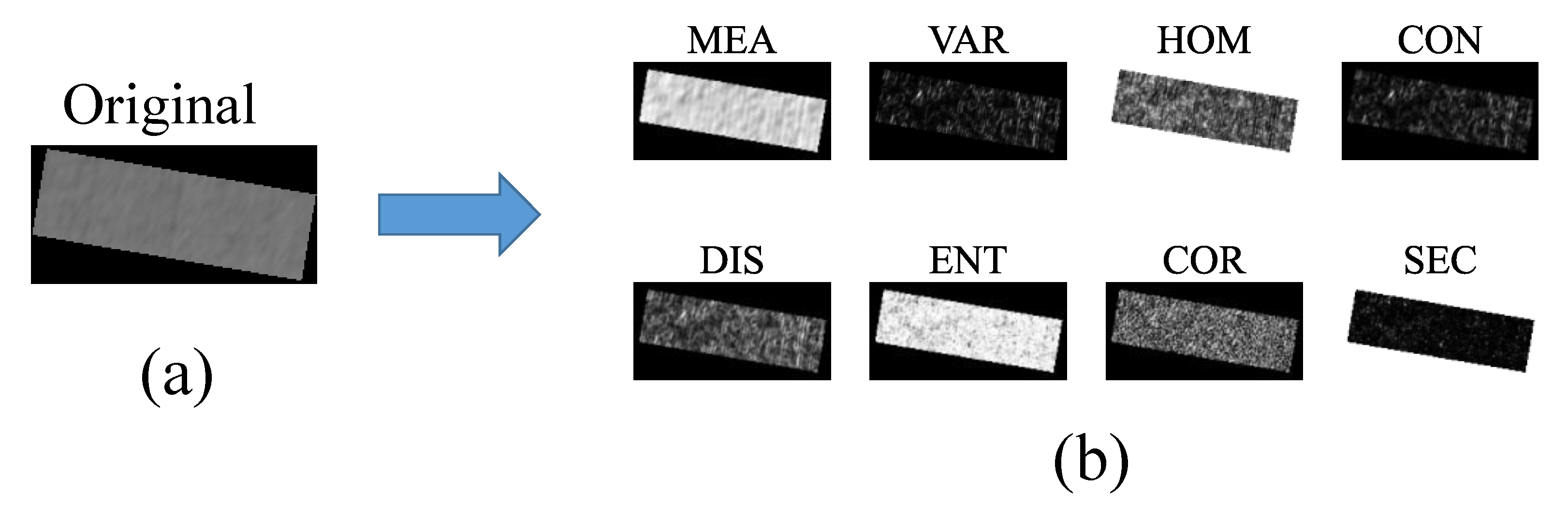
2.3.3. Calculation of TIs

Referring to the VIs formula, several TIs were proposed in related studies (

Table 6. The TIs covered in this article, their abbreviations, and equations.

TIs	Formula
NDTI	$\left(T_1-T_2\right)/\left(T_1+T_2\right)$
DTI	$T_1-T_2$
RDTI	$\left(T_1-T_2\right)/\sqrt{\left(T_1+T_2\right)}$

$T_1$ and $T_2$ represent two random TFVs (i.e., we tested each possible combination of textural features here).

). The renormalized difference texture index (RDTI), which integrates the strengths of both the normalized difference texture index (NDTI) and the difference texture index (DTI) [43], was utilized in this study for rice SPAD estimation.

2.4. Response Association Analysis Metrics

VIs and TIs were generated by calculating linear or non-linear combination formulas. To analyze the relationship between features and assess and screen features, the maximal information coefficient (MIC) was employed in this study. MIC considers not only the linear correlation but also captures the non-linear correlation between features [44,45]. The closer the MIC score is to 1, the better the correlation.

2.5. Model Establishment and Evaluation

The flowchart of this study is shown in Figure 5.

Table 7. Statistics of rice SPAD measurements.

Datasets	Stages	Samples	Min	Max	Mean	Standard Deviation	Coefficient of Variation (%)
Train	Pre-heading	432	30.02	47.4	38.57	3.91	10.14
	Post-heading	288	30.88	45.67	38.85	3.30	8.50
	Whole growth	720	29.40	47.52	38.71	3.78	9.76
Test	Pre-heading	108	29.40	47.52	38.58	4.56	11.81
	Post-heading	72	30.75	44.83	39.00	3.56	9.14
	Whole growth	180	30.49	46.58	38.63	3.84	9.31
Exp. 3	Pre-heading	180	32.07	45.77	38.51	3.39	8.80
	Post-heading	120	30.32	46.80	39.68	3.95	9.96
	Whole growth	300	30.32	46.80	38.98	3.67	9.41

presents the statistics of the SPAD measurements. The data obtained from Exp. 3 was separated from the rest of the data for the purpose of testing the model’s robustness. The data from Exp. 1 and Exp. 2 were mixed as the datasets, which comprised 900 samples, with 540 samples taken during the pre-heading stages and 360 samples taken during the post-heading stages. The datasets were split into training and testing sets with an 8:2 ratio. To prevent any information leakage into the testing set, we performed feature selection using only the training set. The regression model used in this study is random forest (RF), which is a machine learning method based on decision tree algorithms. In RF, multiple decision trees are built on a random subset of training data, and the final prediction is obtained by aggregating the predictions of these individual trees [46,47]. The hyperparameters considered in the model include the number of trees, maximum tree depth, and a minimum number of samples for internal node splitting. Use grid search and cross-validation technology to obtain the best combination of hyperparameters to optimize the model’s performance. The model was evaluated using two metrics: the coefficient of determination ($R^2$) and root mean squared error ($RMSE$). When the value of $R^2$ is larger or the value of $RMSE$ is smaller, it can be considered that the model performs better. Formulae are as follows (1) to (2). This study uses Python and Visual Studio Code for model construction and evaluation.

$$R^2=1-\frac{{\displaystyle \sum _{i=1}^n{\left(y_i-{\widehat{y}}_i\right)}^2}}{{\displaystyle \sum _{i=1}^n{\left(y_i-{\overline{y}}_i\right)}^2}}$$

(1)

$$RMSE=\sqrt{\frac{1}{n}{\displaystyle \sum _{i=1}^n{\left(y_i-{\widehat{y}}_i\right)}^2}}$$

(2)

In the formula, $y_i$ represents the measured value, ${\widehat{y}}_i$ represents the predicted value, ${\overline{y}}_i$ represents the average of the measured values, and n represents the number of test samples.

3. Results

3.1. Estimation of SPAD in Rice with the Spectral VIs

We assessed the MIC between 12 VIs and SPAD values in rice (Figure 6). Previous research has suggested that combining multiple VIs can improve model accuracy. Still, too many input features can increase model complexity. Therefore, we aimed to reduce the number of input features as much as possible without significantly affecting model accuracy. Moreover, we observed strong correlations between certain VIs, which can result in feature redundancy. To balance estimation accuracy and model simplification, we selected two VIs from each dataset.

Ultimately, the combination of ARVI and OSAVI provided the best estimation accuracy for the pre-heading stages. The combination of CIRE and RDVI provided the best estimation accuracy for the post-heading stages. The combination of NDRE and ARVI provided the best estimation accuracy for the whole growth stages. The results of rice SPAD estimation using VIs and RF are presented in

Table 8. The results obtained in this study.

Dataset		Pre-Heading Stages		Post-Heading Stages		Whole Growth Stages
Feature (num)	Metrics	Train	Test	Train	Test	Train	Test
VIs (3)	$R^2$	0.78	0.73	0.81	0.64	0.72	0.70
	$RMSE$	1.8388	2.3630	1.4504	2.1443	1.9978	2.1010
TIs (3)	$R^2$	0.65	0.51	0.55	0.42	0.42	0.36
	$RMSE$	2.3149	3.1783	2.2155	2.7190	2.8687	3.0764
VIs (3) + TIs (3)	$R^2$	0.84	0.79	0.84	0.72	0.86	0.77
	$RMSE$	1.5544	2.0870	1.3384	1.8875	1.3929	1.8462

.

3.2. Estimation of SPAD in Rice with Textural Information

We examined the correlation between 40 TFVs and SPAD values at various kernel sizes (Figure 7). In the pre-heading stages, the MIC of TFVs in the red-edge and NIR bands was significantly better than that in the visible bands. The best TFV was E_diss (7 × 7) with a MIC of 0.39 (Figure 7a). In the post-heading stages, the MIC of TFVs in visible bands was better than that in the red-edge and NIR bands, and the best TFV was B_vari (17 × 17) with a MIC of 0.39 (Figure 7b). However, in the whole growth stages, the TFVs performed poorly in each band, and the best TFV was N_cont (7 × 7) with MIC of 0.27 (Figure 7c). Compared with VIs, the correlation between TFVs and SPAD was poor, and the MICs of the same TFV at different kernel sizes were less distinguishable.

To enhance the correlation between textural information and SPAD, we attempted to construct TIs (RDTIs). We compared the maximum MIC between RDTIs and SPAD for different kernel sizes (Figure 7d). Across all datasets, the trend of curve change was relatively consistent. As the kernel size increased, MIC rapidly increased and became stable when the kernel size reached 7 × 7. We observed that the MIC was close to the best performance in all growth stages when the kernel size was 9 × 9 and 15 × 15. We chose a kernel size of 15 × 15 in all growth stages for this study. During the pre-heading stages, RDTI (N_entr, G_corr) showed the best performance with MIC of 0.48, 23.08% higher than the best TFV. In the post-heading stages, RDTI (B_vari, R_mean) performed the best with a MIC of 0.43, which was 10.26% higher than the best TFV. In the whole growth stages, RDTI (N_entr, G_corr) performed the best with MIC of 0.36, which was 33.33% higher than the best TFV (Figure 8). Our results demonstrate that incorporating TFVs to create RDTIs can effectively enhance the relationship between image texture features and SPAD measurements.

We assessed the MIC between the highest-performing 12 RDTIs and rice SPAD. During the pre-heading, post-heading, and whole growth stages, the MIC values ranged from 0.40 to 0.48, 0.38 to 0.43, and 0.30 to 0.36, respectively. Similar to the process of selecting VIs, we selected two TIs from each dataset and identified the Tis’ combination with the best evaluation index through testing.

The best estimation accuracy for the pre-heading stages was achieved by combining RDTI (N_entr, G_corr) and RDTI (E_entr, G_corr). For the post-heading stages, the combination of RDTI (B_vari, R_mean) and RDTI (B_vari, G_mean) provided the best estimation accuracy. Finally, the combination of RDTI (N_entr, G_corr) and RDTI (B_vari, N_diss) provided the best estimation accuracy for the whole growth stages. The rice SPAD estimation results using TIs and RF are presented in Table 8.

3.3. Combination of VIs and TIs for Estimating SPAD in Rice

The combination of the previously used VIs and TIs was used to build a regression model with RF, and this method yielded the best performance in all growth stages (Table 8) (Figure 9). Compared to using vegetation indices alone, the incorporation of RDTIs resulted in significant improvements in accuracy during testing on datasets. Specifically, during the pre-heading stages, the $R^2$ increased by 8.22% and the $RMSE$ decreased by 11.68%. During the post-heading stages, there was an increase of 12.50% in $R^2$ and a decrease of 11.98% in $RMSE$. In the whole growth stages, there was an increase of 10.00% in $R^2$ and a decrease of 12.13% in $RMSE$. In summary, the combination of VIs and TIs can effectively improve the accuracy of SPAD estimation in rice. We tested the model’s generalizability with the data from Exp. 3, which was conducted in different years and locations; Figure 10 depicts the results obtained from this analysis.

4. Discussion

The 12 VIs we selected in this study showed a moderate correlation with SPAD (Figure 6). We found that VIs constructed from NIR and red-edge spectral bands achieved superior performance compared to others, likely due to their higher sensitivity towards SPAD values. As shown in Table 8, the accuracy of SPAD estimation was observed to be lower during the post-heading stages as compared to the pre-heading stages. This is because VIs tend to saturate under dense vegetation [48,49], and the presence of rice ears can disturb the canopy leaves, leading to inaccurate SPAD estimates. In agriculture, multi-spectral cameras typically have a limited number of bands, which limits the number of VIs that can be synthesized for SPAD estimation. We found that a small number of bands combined into VIs strongly correlated with each other (Figure 6). However, when using multiple features in combination, highly correlated features can provide less information and may even have a negative impact due to multicollinearity. Therefore, we avoided selecting highly correlated features for combination, which further reduced the available information from the spectrum. In summary, it is important to extract additional details from multi-spectral images to enhance the accuracy of SPAD estimation.

The high-resolution images of the rice canopy contain rich textural information. The images mainly consist of complex soils, water, leaves, and stems during the pre-heading stages. During the post-heading stages, the rice canopy coverage increases, and the soil and water become invisible. While rice ears emerge, the canopy structure becomes complex. TFVs in the red-edge and NIR bands performed better for the pre-heading and whole growth stages, while TFVs in the visible bands performed better for the post-heading stages (Figure 7). This indicates that the TFV-sensitive bands changed due to the changes in the canopy structure. Most TFVs showed poor correlation with rice SPAD and were consistent with previous studies on using TFVs to estimate other indicators such as AGB [43]. However, we found that combining two TFVs to construct RDTIs improved the accuracy of rice SPAD estimation compared to using TFVs alone. RDTIs can smooth the canopy structure and reduce the effects of background and solar altitude angles, resulting in a more accurate estimation of various vegetation indicators. This has been demonstrated through research [25,50,51].

The choice of kernel size significantly impacts the accuracy of texture analysis results [52]. A small kernel size can preserve high spatial resolution but may exaggerate intra-kernel variations. Conversely, a large kernel size may not efficiently extract texture information because texture variations are over smoothed [51]. The MICs of the same TFV at different kernel sizes were not significantly different. We compared the maximum MIC between RDTIs and SPAD for different kernel sizes (Figure 7d) and found that the improvement in estimation accuracy was greater in the pre-heading stages as the kernel size increased compared to the 3 × 3 kernel size, possibly because soil and shadows are more distributed among rice plants at this growth stage. A larger kernel can reduce random errors and lead to more accurate estimates of distributions [52]. Canopy cover increases with rice growth, which results in more vegetation being included in the run kernel, so the MIC fluctuated relatively less with increasing kernel size in the post-heading stages.

Chlorophyll and plant photosynthesis are strongly correlated, as plants with higher chlorophyll have a greater photosynthetic capacity and accumulate more photosynthetic products. Previous studies have demonstrated that textural information can effectively estimate rice biomass [27], which is involved in driving SPAD estimation. Moreover, leaves with higher chlorophyll content tend to have a darker color, while leaves with lower chlorophyll content tend to have a lighter color. The combination of these factors results in rice plants with different SPAD values exhibiting distinguishable texture differences in remote sensing images.

VIs provide spectral information on rice canopy, while TIs provide spatial structural information. By combining multiple VIs and TIs, relevant information on rice plant SPAD can be extracted from different perspectives to improve the model’s accuracy. However, although the three experiments were conducted in different fields in this study, the natural conditions were relatively similar. To further verify and improve the model’s generalization performance, it is necessary to include more data from multiple ecological locations and years in future studies. In addition, due to the relatively small amount of data, we did not use deep learning techniques in this study. Future studies will collect more data to explore the performance of deep learning models.

5. Conclusions

This study utilized UAV multi-spectral images to estimate the SPAD values of rice. The main conclusions are as follows: textural information extracted from multi-spectral images can effectively assess the SPAD values of rice. Combining two TFVs to construct RDTIs can further improve the correlation between textural information and SPAD. Compared with using only VIs, incorporating both VIs and TIs to build the model can further improve the accuracy of SPAD estimation across all growth stages. The model also demonstrated good generalizability for calculating rice SPAD in different years and locations. These results have potential applications in precision agriculture and environmental protection.

References

1. Croft, H.; Chen, J.M.; Luo, X.; Bartlett, P.; Chen, B.; Staebler, R.M. Leaf Chlorophyll Content as a Proxy for Leaf Photosynthetic Capacity. Glob. Chang. Biol. 2017, 23, 3513–3524. [Google Scholar] [CrossRef] [PubMed]
2. Cui, B.; Zhao, Q.; Huang, W.; Song, X.; Ye, H.; Zhou, X. A New Integrated Vegetation Index for the Estimation of Winter Wheat Leaf Chlorophyll Content. Remote Sens. 2019, 11, 974. [Google Scholar] [CrossRef]
3. Pinardi, M.; Bresciani, M.; Villa, P.; Cazzaniga, I.; Laini, A.; Tóth, V.; Fadel, A.; Austoni, M.; Lami, A.; Giardino, C. Spatial and Temporal Dynamics of Primary Producers in Shallow Lakes as Seen from Space: Intra-Annual Observations from Sentinel-2A. Limnologica 2018, 72, 32–43. [Google Scholar] [CrossRef]
4. Tischler, Y.K.; Thiessen, E.; Hartung, E. Early Optical Detection of Infection with Brown Rust in Winter Wheat by Chlorophyll Fluorescence Excitation Spectra. Comput. Electron. Agric. 2018, 146, 77–85. [Google Scholar] [CrossRef]
5. Wu, Q.; Zhang, Y.; Zhao, Z.; Xie, M.; Hou, D. Estimation of Relative Chlorophyll Content in Spring Wheat Based on Multi-Temporal UAV Remote Sensing. Agronomy 2023, 13, 211. [Google Scholar] [CrossRef]
6. Yang, X.; Yang, R.; Ye, Y.; Yuan, Z.; Wang, D.; Hua, K. Winter Wheat SPAD Estimation from UAV Hyperspectral Data Using Cluster-Regression Methods. Int. J. Appl. Earth Obs. Geoinf. 2021, 105, 102618. [Google Scholar] [CrossRef]
7. Ban, S.; Liu, W.; Tian, M.; Wang, Q.; Yuan, T.; Chang, Q.; Li, L. Rice Leaf Chlorophyll Content Estimation Using UAV-Based Spectral Images in Different Regions. Agronomy 2022, 12, 2832. [Google Scholar] [CrossRef]
8. Liang, T.; Duan, B.; Luo, X.; Ma, Y.; Yuan, Z.; Zhu, R.; Peng, Y.; Gong, Y.; Fang, S.; Wu, X. Identification of High Nitrogen Use Efficiency Phenotype in Rice (Oryza sativa L.) Through Entire Growth Duration by Unmanned Aerial Vehicle Multispectral Imagery. Front. Plant Sci. 2021, 12, 740414. [Google Scholar] [CrossRef]
9. Wang, Y.; Suarez, L.; Poblete, T.; Gonzalez-Dugo, V.; Ryu, D.; Zarco-Tejada, P.J. Evaluating the Role of Solar-Induced Fluorescence (SIF) and Plant Physiological Traits for Leaf Nitrogen Assessment in Almond Using Airborne Hyperspectral Imagery. Remote Sens. Environ. 2022, 279, 113141. [Google Scholar] [CrossRef]
10. Shcherbak, I.; Millar, N.; Robertson, G.P. Global Metaanalysis of the Nonlinear Response of Soil Nitrous Oxide (N 2 O) Emissions to Fertilizer Nitrogen. Proc. Natl. Acad. Sci. USA 2014, 111, 9199–9204. [Google Scholar] [CrossRef]
11. Zhang, Y.; Hui, J.; Qin, Q.; Sun, Y.; Zhang, T.; Sun, H.; Li, M. Transfer-Learning-Based Approach for Leaf Chlorophyll Content Estimation of Winter Wheat from Hyperspectral Data. Remote Sens. Environ. 2021, 267, 112724. [Google Scholar] [CrossRef]
12. Yao, H.; Qin, R.; Chen, X. Unmanned Aerial Vehicle for Remote Sensing Applications—A Review. Remote Sens. 2019, 11, 1443. [Google Scholar] [CrossRef]
13. Zhao, C. Unmanned Aerial Vehicle Remote Sensing for Field-Based Crop Phenotyping: Current Status and Perspectives. Front. Plant Sci. 2017, 8, 26. [Google Scholar]
14. Acorsi, M.G.; das Dores Abati Miranda, F.; Martello, M.; Smaniotto, D.A.; Sartor, L.R. Estimating Biomass of Black Oat Using UAV-Based RGB Imaging. Agronomy 2019, 9, 344. [Google Scholar] [CrossRef]
15. Lu, W.; Okayama, T.; Komatsuzaki, M. Rice Height Monitoring between Different Estimation Models Using UAV Photogrammetry and Multispectral Technology. Remote Sens. 2021, 14, 78. [Google Scholar] [CrossRef]
16. Kayad, A.; Sozzi, M.; Paraforos, D.S.; Rodrigues, F.A.; Cohen, Y.; Fountas, S.; Francisco, M.-J.; Pezzuolo, A.; Grigolato, S.; Marinello, F. How Many Gigabytes per Hectare Are Available in the Digital Agriculture Era? A Digitization Footprint Estimation. Comput. Electron. Agric. 2022, 198, 107080. [Google Scholar] [CrossRef]
17. Verger, A.; Vigneau, N.; Chéron, C.; Gilliot, J.-M.; Comar, A.; Baret, F. Green Area Index from an Unmanned Aerial System over Wheat and Rapeseed Crops. Remote Sens. Environ. 2014, 152, 654–664. [Google Scholar] [CrossRef]
18. Zhou, X.; Zheng, H.B.; Xu, X.Q.; He, J.Y.; Ge, X.K.; Yao, X.; Cheng, T.; Zhu, Y.; Cao, W.X.; Tian, Y.C. Predicting Grain Yield in Rice Using Multi-Temporal Vegetation Indices from UAV-Based Multispectral and Digital Imagery. ISPRS J. Photogramm. Remote Sens. 2017, 130, 246–255. [Google Scholar] [CrossRef]
19. Yang, H.; Hu, Y.; Zheng, Z.; Qiao, Y.; Zhang, K.; Guo, T.; Chen, J. Estimation of Potato Chlorophyll Content from UAV Multispectral Images with Stacking Ensemble Algorithm. Agronomy 2022, 12, 2318. [Google Scholar] [CrossRef]
20. Zhang, S.; Zhao, G.; Lang, K.; Su, B.; Chen, X.; Xi, X.; Zhang, H. Integrated Satellite, Unmanned Aerial Vehicle (UAV) and Ground Inversion of the SPAD of Winter Wheat in the Reviving Stage. Sensors 2019, 19, 1485. [Google Scholar] [CrossRef]
21. Yang, K.; Gong, Y.; Fang, S.; Duan, B.; Yuan, N.; Peng, Y.; Wu, X.; Zhu, R. Combining Spectral and Texture Features of UAV Images for the Remote Estimation of Rice LAI throughout the Entire Growing Season. Remote Sens. 2021, 13, 3001. [Google Scholar] [CrossRef]
22. Jiang, X.; Zhen, J.; Miao, J.; Zhao, D.; Shen, Z.; Jiang, J.; Gao, C.; Wu, G.; Wang, J. Newly-Developed Three-Band Hyperspectral Vegetation Index for Estimating Leaf Relative Chlorophyll Content of Mangrove under Different Severities of Pest and Disease. Ecol. Indic. 2022, 140, 108978. [Google Scholar] [CrossRef]
23. Kim, H.-O.; Yeom, J.-M. Effect of Red-Edge and Texture Features for Object-Based Paddy Rice Crop Classification Using RapidEye Multi-Spectral Satellite Image Data. Int. J. Remote Sens. 2014, 35, 7046–7068. [Google Scholar] [CrossRef]
24. Dube, T.; Mutanga, O. Investigating the Robustness of the New Landsat-8 Operational Land Imager Derived Texture Metrics in Estimating Plantation Forest Aboveground Biomass in Resource Constrained Areas. ISPRS J. Photogramm. Remote Sens. 2015, 108, 12–32. [Google Scholar] [CrossRef]
25. Yue, J.; Yang, G.; Tian, Q.; Feng, H.; Xu, K.; Zhou, C. Estimate of Winter-Wheat above-Ground Biomass Based on UAV Ultrahigh-Ground-Resolution Image Textures and Vegetation Indices. ISPRS J. Photogramm. Remote Sens. 2019, 150, 226–244. [Google Scholar] [CrossRef]
26. Yang, Q.; Shi, L.; Han, J.; Chen, Z.; Yu, J. A VI-Based Phenology Adaptation Approach for Rice Crop Monitoring Using UAV Multispectral Images. Field Crops Res. 2022, 277, 108419. [Google Scholar] [CrossRef]
27. Zheng, H.; Cheng, T.; Zhou, M.; Li, D.; Yao, X.; Tian, Y.; Cao, W.; Zhu, Y. Improved Estimation of Rice Aboveground Biomass Combining Textural and Spectral Analysis of UAV Imagery. Precis. Agric. 2019, 20, 611–629. [Google Scholar] [CrossRef]
28. Tucker, C.J. Red and Photographic Infrared Linear Combinations for Monitoring Vegetation. Remote Sens. Environ. 1979, 8, 127–150. [Google Scholar] [CrossRef]
29. Gitelson, A.A.; Kaufman, Y.J.; Merzlyak, M.N. Use of a Green Channel in Remote Sensing of Global Vegetation from EOS-MODIS. Remote Sens. Environ. 1996, 58, 289–298. [Google Scholar] [CrossRef]
30. Gamon, J.A.; Surfus, J.S. Assessing Leaf Pigment Content and Activity with a Reflectometer. New Phytol 1999, 143, 105–117. [Google Scholar] [CrossRef]
31. Xiao, Y.; Zhao, W.; Zhou, D.; Gong, H. Sensitivity Analysis of Vegetation Reflectance to Biochemical and Biophysical Variables at Leaf, Canopy, and Regional Scales. IEEE Trans. Geosci. Remote Sens. 2014, 52, 11. [Google Scholar] [CrossRef]
32. Rondeaux, G.; Steven, M.; Baret, F. Optimization of Soil-Adjusted Vegetation Indices. Remote Sens. Environ. 1996, 55, 95–107. [Google Scholar] [CrossRef]
33. Jordan, C.F. Derivation of Leaf-Area Index from Quality of Light on the Forest Floor. Ecology 1969, 50, 663–666. [Google Scholar] [CrossRef]
34. Blackburn, G.A. Quantifying Chlorophylls and Caroteniods at Leaf and Canopy Scales: An Evaluation of Some Hyperspectral Approaches. Remote Sens. Environ. 1998, 66, 273–285. [Google Scholar] [CrossRef]
35. Tanr, D. Atmospherically Resistant Vegetation Index (ARVI) for EOS-MODIS. IEEE Trans. Geosci. Remote Sens. 1992, 30, 261–270. [Google Scholar]
36. Huete, A.; Didan, K.; Miura, T.; Rodriguez, E.P.; Gao, X.; Ferreira, L.G. Overview of the Radiometric and Biophysical Performance of the MODIS Vegetation Indices. Remote Sens. Environ. 2002, 83, 195–213. [Google Scholar] [CrossRef]
37. Gitelson, A.A.; Viña, A.; Arkebauer, T.J.; Rundquist, D.C.; Keydan, G.; Leavitt, B. Remote Estimation of Leaf Area Index and Green Leaf Biomass in Maize Canopies: Remote estimation of leaf area index. Geophys. Res. Lett. 2003, 30, 52-1–52-4. [Google Scholar] [CrossRef]
38. Roujean, J.-L.; Breon, F.-M. Estimating PAR Absorbed by Vegetation from Bidirectional Reflectance Measurements. Remote Sens. Environ. 1995, 51, 375–384. [Google Scholar] [CrossRef]
39. Huete, A.R. A Soil-Adjusted Vegetation Index (SAVI). Remote Sens. Environ. 1988, 25, 295–309. [Google Scholar] [CrossRef]
40. Haralick, R.M.; Shanmugam, K.; Dinstein, I. Textural Features for Image Classification. IEEE Trans. Syst. Man Cybern. 1973, SMC-3, 610–621. [Google Scholar] [CrossRef]
41. Hall-Beyer, M. Practical Guidelines for Choosing GLCM Textures to Use in Landscape Classification Tasks over a Range of Moderate Spatial Scales. Int. J. Remote Sens. 2017, 38, 1312–1338. [Google Scholar] [CrossRef]
42. Hall-Beyer, M. GLCM Texture: A Tutorial v. 3.0 March 2017. Available online: http://hdl.handle.net/1880/51900 (accessed on 15 June 2022).
43. Lu, J.; Eitel, J.U.H.; Engels, M.; Zhu, J.; Ma, Y.; Liao, F.; Zheng, H.; Wang, X.; Yao, X.; Cheng, T.; et al. Improving Unmanned Aerial Vehicle (UAV) Remote Sensing of Rice Plant Potassium Accumulation by Fusing Spectral and Textural Information. Int. J. Appl. Earth Obs. Geoinf. 2021, 104, 102592. [Google Scholar] [CrossRef]
44. Shao, F.; Liu, H. The Theoretical and Experimental Analysis of the Maximal Information Coefficient Approximate Algorithm. J. Syst. Sci. Inf. 2021, 9, 95–104. [Google Scholar] [CrossRef]
45. Qiao, L.; Tang, W.; Gao, D.; Zhao, R.; An, L.; Li, M.; Sun, H.; Song, D. UAV-Based Chlorophyll Content Estimation by Evaluating Vegetation Index Responses under Different Crop Coverages. Comput. Electron. Agric. 2022, 196, 106775. [Google Scholar] [CrossRef]
46. Zhang, C.; Ma, Y. (Eds.) Ensemble Machine Learning; Springer: Boston, MA, USA, 2012; ISBN 978-1-4419-9325-0. [Google Scholar]
47. Zhu, W.; Rezaei, E.E.; Nouri, H.; Sun, Z.; Li, J.; Yu, D.; Siebert, S. UAV-Based Indicators of Crop Growth Are Robust for Distinct Water and Nutrient Management but Vary between Crop Development Phases. Field Crops Res. 2022, 284, 108582. [Google Scholar] [CrossRef]
48. Fu, Y.; Yang, G.; Wang, J.; Song, X.; Feng, H. Winter Wheat Biomass Estimation Based on Spectral Indices, Band Depth Analysis and Partial Least Squares Regression Using Hyperspectral Measurements. Comput. Electron. Agric. 2014, 100, 51–59. [Google Scholar] [CrossRef]
49. Wan, L.; Cen, H.; Zhu, J.; Zhang, J.; Zhu, Y.; Sun, D.; Du, X.; Zhai, L.; Weng, H.; Li, Y.; et al. Grain Yield Prediction of Rice Using Multi-Temporal UAV-Based RGB and Multispectral Images and Model Transfer—A Case Study of Small Farmlands in the South of China. Agric. For. Meteorol. 2020, 291, 108096. [Google Scholar] [CrossRef]
50. Eckert, S. Improved Forest Biomass and Carbon Estimations Using Texture Measures from WorldView-2 Satellite Data. Remote Sens. 2012, 20, 810–829. [Google Scholar] [CrossRef]
51. Sarker, L.R.; Nichol, J.E. Improved Forest Biomass Estimates Using ALOS AVNIR-2 Texture Indices. Remote Sens. Environ. 2011, 115, 968–977. [Google Scholar] [CrossRef]
52. Franklin, S.E.; Hall, R.J.; Moskal, L.M.; Maudie, A.J.; Lavigne, M.B. Incorporating Texture into Classification of Forest Species Composition from Airborne Multispectral Images. Int. J. Remote Sens. 2000, 21, 61–79. [Google Scholar] [CrossRef]
Figure 1. The geographical location of the base (a), the field of Exp. 1 (c), Exp. 2 (d), Exp. 3 (e), and the layout of the experimental plots (b).
Agronomy 13 01541 g001
Figure 2. The appearance of rice throughout the whole growth period.
Agronomy 13 01541 g002
Figure 3. Segmentation of the experimental plots.
Agronomy 13 01541 g003
Figure 4. The original image (a) of the plot was computed to generate the TFVs image (b) by removing the boundary.
Agronomy 13 01541 g004
Figure 5. Flowchart of this study.
Agronomy 13 01541 g005
Figure 6. Correlation matrix (MIC) of VIs for the pre-heading (a), post-heading (b), and whole growth stages (c).
Agronomy 13 01541 g006
Figure 7. Analysis of the MIC of TFVs and SPAD in different kernel sizes for the pre-heading (a), post-heading (b), and whole growth stages (c). Eight TFVs are extracted for each band in the same order as in Table 5. The order of the bands is blue (B), green (G), red (R), red-edge (E), and NIR (N) bands, with a total of 40 TFVs, and the order is numbered 1–40. The RDTI and SPAD of MIC for different kernel sizes were analyzed during the pre-heading, post-heading, and the whole growth stage, represented by lines 1, 2, and 3, respectively (d).
Agronomy 13 01541 g007
Figure 8. Any element in the figure represents the MIC of RDTI and SPAD for the pre-heading (a), post-heading (b), and whole growth stages (c). RDTIs were calculated from the two TFVs corresponding to their horizontal and vertical coordinates. For interpretation of the labels of the x and y axes, please refer to Figure 7.
Agronomy 13 01541 g008
Figure 9. Test results of SPAD estimation in test datasets using the combined VIs and TIs with the RF model for the pre-heading (a), post-heading (b), and whole growth stages (c), with the red line as a 1:1 straight line.
Agronomy 13 01541 g009
Figure 10. Test results of SPAD estimation in Exp. 3 datasets using the combined VIs and TIs, and RF model for the pre-heading (a), post-heading (b), and whole growth stages (c), with the red line as a 1:1 straight line.
Agronomy 13 01541 g010