YOLOv7-GCA: A Lightweight and High-Performance Model for Pepper Disease Detection

Abstract

Existing disease detection models for deep learning-based monitoring and prevention of pepper diseases face challenges in accurately identifying and preventing diseases due to inter-crop occlusion and various complex backgrounds. To address this issue, we propose a modified YOLOv7-GCA model based on YOLOv7 for pepper disease detection, which can effectively overcome these challenges. The model introduces three key enhancements: Firstly, lightweight GhostNetV2 is used as the feature extraction network of the model to improve the detection speed. Secondly, the Cascading fusion network (CFNet) replaces the original feature fusion network, which improves the expression ability of the model in complex backgrounds and realizes multi-scale feature extraction and fusion. Finally, the Convolutional Block Attention Module (CBAM) is introduced to focus on the important features in the images and improve the accuracy and robustness of the model. This study uses the collected dataset, which was processed to construct a dataset of 1259 images with four types of pepper diseases: anthracnose, bacterial diseases, umbilical rot, and viral diseases. We applied data augmentation to the collected dataset, and then experimental verification was carried out on this dataset. The experimental results demonstrate that the YOLOv7-GCA model reduces the parameter count by 34.3% compared to the YOLOv7 original model while improving 13.4% in mAP and 124 frames/s in detection speed. Additionally, the model size was reduced from 74.8 MB to 46.9 MB, which facilitates the deployment of the model on mobile devices. When compared to the other seven mainstream detection models, it was indicated that the YOLOv7-GCA model achieved a balance between speed, model size, and accuracy. This model proves to be a high-performance and lightweight pepper disease detection solution that can provide accurate and timely diagnosis results for farmers and researchers.

1. Introduction

Pepper (Capsicum annuum L.) is one of the most economical and versatile agricultural vegetables in the world [1]. It has wide applications in medicine, cosmetics, and other fields; it is also an essential ingredient in our cuisine, and it also contributes to dietary nutrition [2]. However, pepper plants are susceptible to various diseases during their growth process due to climate change, pest invasion, and natural disasters. These diseases can reduce the yield and quality of pepper crops, causing serious economic losses to farmers [3,4]. Therefore, timely and accurate identification of pepper diseases is crucial for effective disease control and the sustainable development of the pepper industry.

Currently, manual observation and empirical judgment are the main sources of the identification of pepper diseases. This method is not only labor-intensive and time-wasting but also prone to misjudgment and omission, which cannot meet the requirements of large-scale, fast, and accurate identification [5]. Therefore, the use of intelligent terminal equipment to identify pepper pests has become a promising solution [6]. To ensure the efficiency and quality of device detection [7], accurate and real-time detection of pepper diseases is crucial. Agricultural plant disease identification is a significant research topic, and machine learning (ML) plays a vital role in it. Traditional machine learning methods usually require manual feature extraction, such as color, texture, and shape, and then use classifiers for identification. For example, Zhang et al. [8] used HSI, YUV, and grayscale models to extract 38 features and used a support vector machine (SVM) classifier to identify three diseases of apple leaves, with an accuracy of more than 90%. Soarov et al. [9] used Otsu threshold segmentation and histogram equalization to process data images and then used SVM for classification, achieving an accuracy of 96% for apple leaf disease identification. Zhang et al. [10] used the K-means clustering algorithm to segment the images, obtaining the shape and color features of pest information, and had a good recognition effect on the 7 major diseases of cucumber, with a total accuracy of 85.7%. However, traditional machine learning methods also have some limitations, such as requiring a single experimental background, and lacking effective interaction and feedback mechanisms, resulting in insufficient accuracy and robustness of the algorithm. To overcome these problems, some researchers started to use deep learning-based methods, using convolutional neural networks (CNN) and other models to directly learn features from images without human intervention, improving the efficiency and accuracy of identification. For example, Ashutosh Kumard et al. [11] used CNN, Bayesian-optimized SVM, and a random forest classifier based on hybrid features to perform plant leaf disease detection, and the results showed that CNN achieved the highest accuracy of 96.1% in detecting leaf disease in apple, corn, potato, tomato, and rice plants. Nurul Nabilah et al. [12] compared the pepper pest features extracted by the traditional ML method with the deep learning-based methods, which outperformed the traditional feature-based methods.

Moreover, with the development of computer vision and artificial intelligence, deep learning (DL) has become a research hotspot in the field of agricultural plant protection, such as plant disease identification and pest range assessment [13]. The object detection algorithm can achieve rapid, accurate, and non-destructive detection [14] of pepper diseases and meet the requirements of real-time detection of pepper diseases.

Recently, deep learning-based object detection methods have made remarkable progress in agriculture. Various deep learning models have been applied to the task of plant disease identification, such as Faster R-CNN, SSD, and RetinaNet. These models have achieved good results in detecting diseases on soybean leaves [15], apple leaves [16], and tea leaves [17], respectively. Among them, the YOLO (You Only Look Once) series of algorithms, as a classic of the one-stage algorithm, have attracted wide attention for their efficient, real-time, and robust characteristics. YOLO transforms the object detection problem into a regression problem, outputs the object position and category information [18] through a single forward propagation, avoiding the complex bounding box generation and selection process in the traditional method. It significantly surpasses the inference speed of the two-stage algorithm, which gives it certain advantages. So the YOLO series plays an important role in agriculture. The YOLO series algorithms are a breakthrough in the field of plant disease identification as they overcome the challenges that other object detection algorithms face. These challenges include high model complexity, unsatisfactory detection of small and dense objects, and a lack of generalization ability across crops in iterative optimization.

Although the YOLO series models propose some effective solutions for the problems above [19,20], it is necessary to optimize the balance of accuracy, speed, and lightweightness. A large number of experiments have been conducted around these three aspects to optimize the existing YOLO model. Liu Jun et al. [21] optimized the feature layer of the image pyramid to realize multi-scale feature detection in the YOLOv3 model, improving the detection precision and speed of the YOLOv3 model and accurately and quickly detecting the location and category of tomato diseases and insect pests. Xuewei Wang et al. [22] proposed a novel YOLO-ense that solved the problem of detecting tomato anomalies by adding densely connected modules, the K-means algorithm, and changing the training strategy with improved precision and speed, achieving 96.41% and 20.28 ms, respectively. YOLOv3 is a relatively mature object detection scheme, but its model computational complexity is relatively high, limiting the improvement effect. Li Dawei et al. [23] proposed the YOLO-JD model to identify jute diseases. Based on YOLOv4, they integrated three new modules. Although the mAP was 96.63% good in terms of jute diseases and pests, the size of the model and detection speed were not well explained. Helong Yu et al. [24] based on the YOLOv5s model and adopted the sample conversion method, which reduced the false positive rate and underreporting rate by eliminating redundant bounding boxes. They achieved a good balance between the detection precision and model size of soybean insect pests, reaching 95.24% mAP when the model file size was only 15.1 MB. Xue Zhenyang et al. [25] used ACmix, CBM, RFB, GCNet, and other modules to improve the YOLOv5 model, which greatly improved the precision and lightweight of the original model in the identification of tea pests. Weishi Xu et al. [26] proposed the problem of an accurate and lightweight apple leaf disease detection model (ALAD-YOLO) based on YOLOv5s by introducing MobileNetV3, CA, and Ghost modules to improve YOLOv5s, shrinking the model volume while maintaining high detection precision. It can be seen that lightweight and precision have become the focus of improvement in the process of improving the YOLOv5 model. Due to the limited model structure, it cannot take into account the requirements of real-time detection in special scenarios. Yang Shuai et al. [27] tackled the issue of swift maize pests, adding the CSPResNeXt-50 module and VoVGSCSP module to enhance YOLOv7, and offer precise and timely pest detection and identification for maize plants. However, the results show that the improved model is only 10 frame/s higher than the original YOLOv7 model in terms of detection speed, and there is still a lot of room for improvement. Liangquan Jia et al. [28] developed a new rice disease and pest identification model based on the improved YOLOv7 algorithm, which enhanced the advantages of high performance, lightweight and lightweight by improving the modules of MobileNetV3, CA, and SIOU. The response speed was up to 87.7 ms, but the model was the result of a trade-off on the premise of a 0.9% decrease in the mAP index. To sum up, many excellent modules and network structures have been proposed for the identification of various crop diseases and insect pests, but most of them are still in the theoretical stage and lack practical application. Therefore, further improvements are needed to complete the identification of pepper diseases in different backgrounds in the field.

In this paper, we aim to address the problem of the insufficient performance of pepper disease detection in the field and in various environments. We propose a high-performance and lightweight pepper disease detection model based on the improved YOLOv7, which can accurately and quickly identify pepper diseases and help to realize the intelligence of pepper agriculture. The main contributions of this study are as follows:

(1)

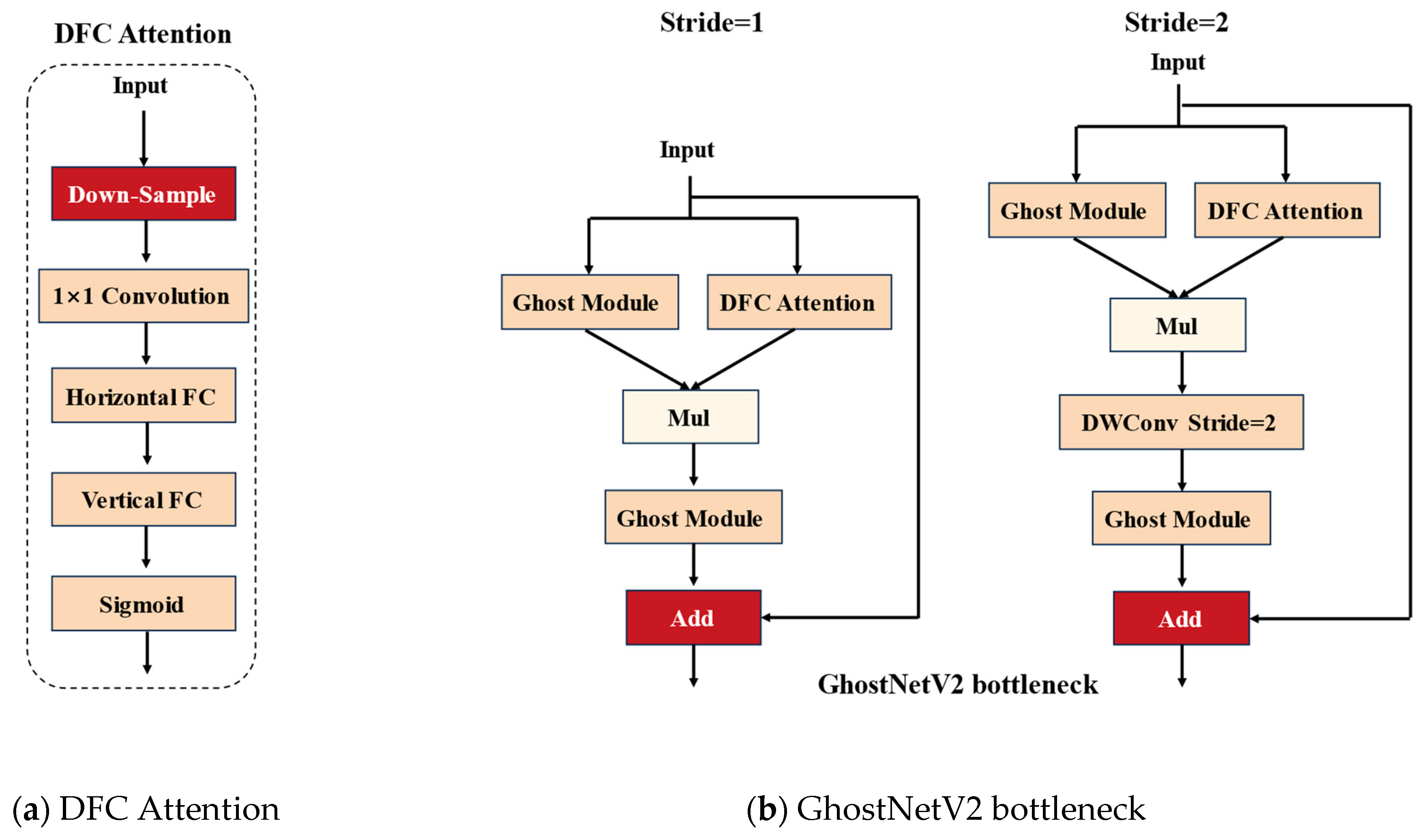
Incorporating GhostNetV2 [29] as the backbone network, which can reduce the number of parameters caused by unnecessary feature computation, enhance the detection speed, and reduce the computing cost while ensuring high performance.

(2)

To tackle the problem of complex backgrounds, Cascade Fusion Network (CFNet) [30] is integrated as a feature fusion network, which enables more parameters to be used for feature fusion and improves the performance of the model.

(3)

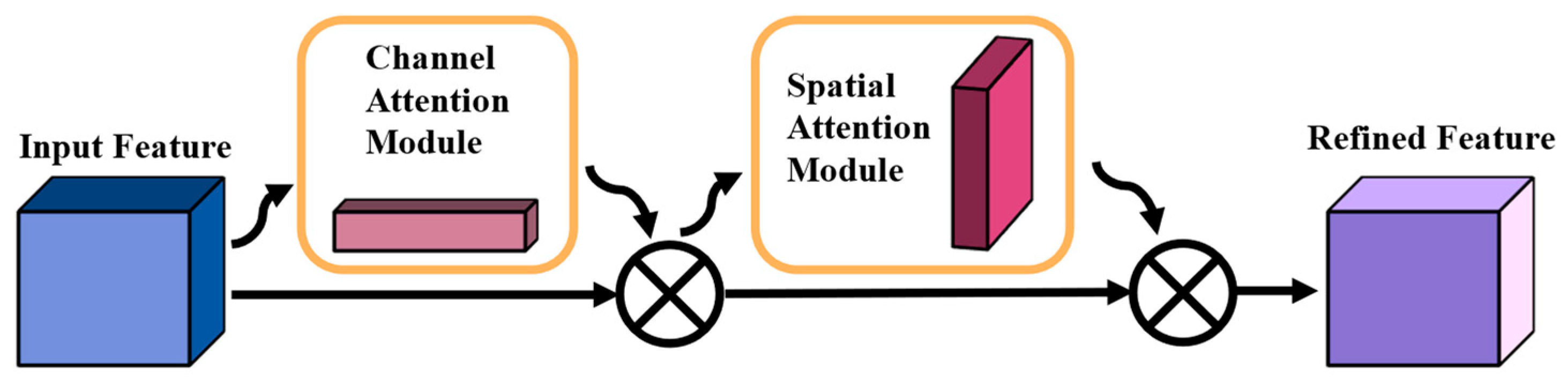
The convolutional Block Attention Module (CBAM) [31] is introduced to improve the model by emphasizing only key features. In this way, the model can better distinguish the features of different channels and better capture key information in space, thus improving its feature extraction ability.

2. Materials and Methods

2.1. Materials

2.1.1. Data Acquisition

This study focused on the pepper plants from a plantation base in Conghua District (113.48817° N, 23.43718° E), Guangzhou City, Guangdong Province. We collected RGB images of four pepper diseases, as shown in

Table 1. Characteristics of the four pepper leaf and fruit diseases.

Name	Number	Label	Characteristics	Picture
Anthracnose_leaf	232	Anthr_leaf	At the beginning of the disease, the leaves showed chlorotic water stain spots, brown round spots with the aggravation of the disease, and small black spots on the late spots.
Anthracnose_fruit	216	Anthr_fruit	At the beginning of the disease, the fruit has irregular or oblong brown spots, the surface of the fruit is sunken, with the aggravation of the disease, the disease spots are dry, and the spots are membranous and easy to rupture.
Viral diseases_leaf	251	Viral_leaf	The diseased leaves are slightly chlorotic, and also show the diseased leaves and wrinkled deformity, and the leaf surface is uneven. When severe, the leaves become hard and thick, the leaf edge curls upward, and the young leaves show linear leaves.
Viral diseases_fruit	187	Viral_fruit	Fruit characteristics of virus disease: the fruit faded to yellow brown, with brown necrotic spots on the fruit.
Bacterial diseases_leaf	163	Bacter_leaf	After leaf disease, the initial symptoms are small green-yellow spots, water stains that gradually expand and deepen, and brown or rusty, membranous. The spots expand rapidly until most of the leaves of the pepper plants wither and fall.
Umbilical rot	210	Umb_rot	Pepper umbilical rot mainly occurs near the umbilicus of the fruit. At the early stage of the disease, water-stained green spots are formed in the umbilicus of the young fruit and green fruit. With the development of the fruit, the disease is grayish brown or white flat depression, and the disease can expand to half the fruit.

, and constructed a dataset for pepper diseases detection. The dataset contains 1259 images of 448 anthracnoses, 438 viral diseases, 163 bacterial diseases, and 210 umbilical rot diseases. The dataset covers different scenarios as well as different shooting angles and distances. The images in the dataset have the following characteristics:

(1)

The image resolution is 3072 × 4093, and the shooting device is a Xiaomi13 smartphone (Xiaomi Corporation, Beijing, China). The maximum pixel value of the camera is 50 million;

(2)

The images contain pepper fruits and leaves with different diseases, but the umbilical rot has only the disease fruit image, and the bacterial disease only the disease has leaf image;

(3)

There are some complex background factors in the image, such as occlusion, overlap, blur, and small objects.

As shown in

Table 2. The partitioning of the dataset.

	Name	Proportion	Number of Pictures	Number of Labels
Dataset	Training Set	80%	1007	2066
	Validation Set	10%	126	267
	Test Set	10%	126	255
Total		100%	1259	2588

, there were 1259 pepper images in the dataset, of which 2588 diseased pepper fruits or leaves were captured and divided into training, test, and validation sets at a ratio of 80/10/10. The training set consisted of 1007 images containing 2066 diseases pepper labels, and the test set contained 126 images with 267 diseases pepper labels, and the remaining 126 images contained 255 diseases pepper labels to constitute the validation set. In addition, 52% of the images in the dataset belong to the category [32] of small objects, i.e., the characteristics of diseases in pepper are less than 32 × 32 pixels, these images are mainly pepper with viral and bacterial diseases; the remaining 48% of the images belong to the large object category, mainly pepper with anthracnose and umbilical rot. All the datasets were stored in JPG format.

2.1.2. Data Augmentation

To enhance the model’s generalization and robustness, we performed data augmentation on the dataset to accommodate different training requirements, which can better extract image features, avoid overfitting, and cope with various complex phenomena existing in the real environment. We augmented the original dataset with 8 different data augmentation methods, namely: random contrast adjustment [33], Cutout [34], random rotation (–45° to +45°), Gaussian blur [35], salt and pepper noise [36], scale [37], and random cropping [38]. Random contrast adjustment can reduce the brightness deviation caused by environmental illumination change and sensor difference; Cutout can randomly select multiple fixed-size square areas to fill with zero pixel value to simulate the occlusion phenomenon; random rotation can increase the directional diversity of the image; Gaussian blur and noise can simulate the image degradation and improve the model’s ability to optimize for background blur and photo quality difference; zoom and random cropping can change the size and proportion of the image to enhance the model’s ability to detect small and overlapping targets.

In addition, we adopted the mosaic data augmentation technique [39] from the YOLO network, which randomly cropped and merged four images into one image to enlarge the image dataset for model training, thereby enhancing the network’s learnable content. The specific data processing steps are as follows: During the training phase, we adjusted the HSV color space value to 0.015, 0.7, and 0.4 to improve the tone, saturation, and brightness of the input image, and minimize the impact of occlusion, lighting, and shadow factors. Subsequently, we scaled the images with a random factor of 0.8 and flipped each image with a probability of 0.5. Then, we took the four processed images and performed the mosaic operation. We extracted the fixed area of the four images in a matrix and combined them into a new image to finish the fusion of the image and the object box. This method can diversify the background of the detected object so that the model can concentrate on general scenes and boost the model’s generalization ability, make it suitable for scenarios where pepper leaves or fruits may occur on branches, ground, or experimental tables. Figure 1 illustrates an example of the image augmentation used in this experiment.

To simulate the complex environment and eliminate the blocking interference between the leaves of pepper fruits, we performed the central normalization operation on the images. Figure 1 shows the results of the data augmentation method. The final training set consisted of 12,590 images for object detection, which included 11,331 augmented images and 1259 original images with no overlap between the training and test sets. We used LabelImg (Version 1.8.6) [40] as the label software, with rectangular label boxes and English label names. There were 6 classes: Anthr_fruit, Anthr_leaf, Bacter_leaf, Umb_rot, Viral_fruit, and Viral_leaf. We generated the corresponding XML tag files and completed the overall construction of the dataset according to the COCO dataset [32].

2.2. YOLOv7-GCA Construction

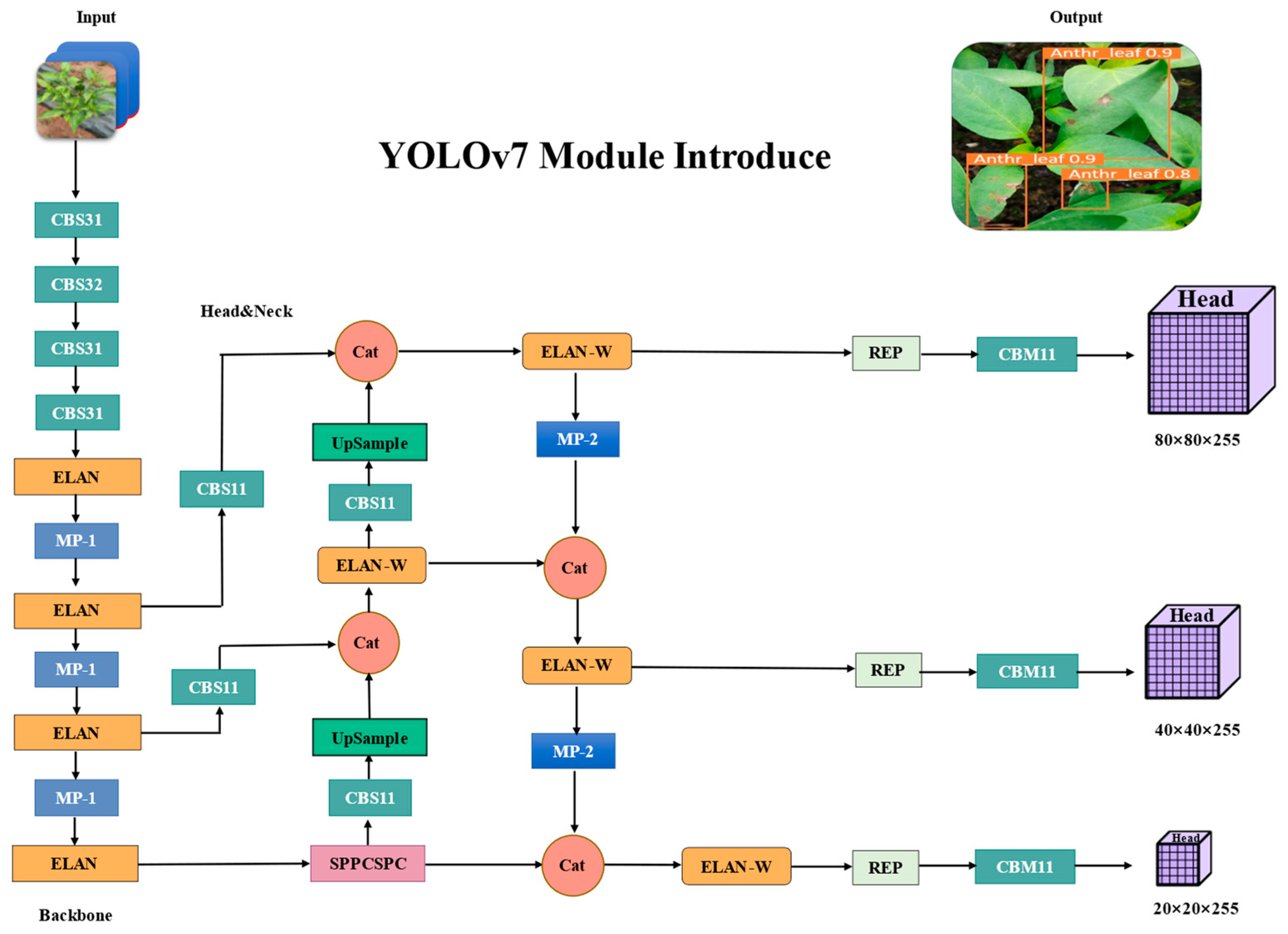
2.2.1. YOLOv7: Expand Efficient Layer Aggregation Networks

YOLOv7 [41] is an advanced object detection model of the YOLO series. Since the YOLO [42] network model was proposed in 2016, the single-stage detection algorithm has first appeared in the human field of view. It overcomes the drawback of low inference speed in the two-stage detection network and preserves on detection accuracy. In 2022, YOLOv7 was born. Compared with YOLOv4 [39], it was mainly improved in the model structure, heavy parameter module [43], label allocation mode, and model scale [44]. Innovatively proposed the Extended Efficient Layer Aggregation Network (E-ELAN) architecture that can improve the self-learning ability of the network without destroying the original gradient path.

The YOLOv7 model is a representative single-level object detection algorithm, and its network structure diagram is shown in Figure 2. The network consists of four parts: image input, backbone network, feature fusion network, and output. Image input resizes all the input images to a consistent size and passes them to the backbone network. The backbone network [41] is composed of multiple CBS convolution layers, ELAN convolution layers, and MPConv [45] to extract image features of different scales. The feature fusion network is composed of the path aggregation feature pyramid network (PAFPN) [46], which integrates features of different scales and introduces bottom-up paths to transfer the information from the bottom. The output consists of three feature maps of different scales, each using 1 × 1 convolutional layers to predict confidence, classification, and bounding box. To meet the demands of real-time and accuracy for field pepper diseases detection models and balance well between detection speed and accuracy, we chose YOLOv7 as the benchmark model.

2.2.2. Lightweight Feature Extraction Module GhostNetV2

The ELAN module implementation improves the learning ability of the network without destroying the original gradient path, but it is only based on traditional convolution operations, which can only capture local information and are susceptible to redundant features. To meet the requirement of high efficiency in field pepper diseases detection, we designed a lightweight feature extraction structure on the backbone network of the original YOLOv7 model. We replaced the ELAN structure in the original network model with GhostNetV2 as a more efficient backbone network for feature extraction.

GhostNetV2, as shown in Figure 3b, uses two Ghost modules and one DFC attention module. The first Ghost module and the DFC attention module are processed and multiplied simultaneously, enhancing the extension feature and being input into the second Ghost module. The second Ghost module takes the boosted features and produces the output features to achieve improved model feature extraction performance. The GhostNetV2 module reduces the number of parameters effectively and enhances the expression ability of the model. This design successfully decreases the coupling between model expressivity and capacity [47], solving the problem of model overfitting during training or inadequate generalization during testing.

DFC is a hardware-friendly attention mechanism that reduces FLOPs [29] by 75% compared to the convolution module GhostNet [48] by reducing feature size in the horizontal and vertical directions and sets the Sigmoid function in the downsampling layer to improve inference speed. Figure 3a shows the schematic diagram of the structure of the DFC attention module. This module can capture the dependence between long-distance pixels, improve the expression and diversity of feature maps, and capture global information well while taking into account speed, thus improving the model detection performance.

The Ghost module produces substantial feature mapping at a low operational cost. It can typically substitute the standard convolution with these two steps: First, the input features $X\in R^{H\times W\times C}$ and 1 × 1 dot states are convolved to generate part of the output features:

$$Y \prime =X\ast F_{1\times 1}$$

(1)

where, $\ast$ represents the convolution operation. $F_{1\times 1}$ refers to the point-wise convolution and $Y \prime \in R^{H\times W\times C_{out}^{ \prime }}$ is partial output features, and they generally have smaller sizes compared to the original output.

The second step is a cheap operation, which is not achieved by conventional convolution, but by a simple linear transformation to generate more feature maps. The two parts of these features are concatenated along the channel dimension, i.e.,

$$Y=Concat\left(\right[Y \prime , Y \prime \ast F_{dp}\left]\right)$$

(2)

In Equation (2), $F_{dp}$ refers to the depth-wise separable convolution and $Y\in R^{H\times W\times C_{out}}$ is the final output feature.

The Ghost module is a convolution module that reduces the computational cost by splitting the standard convolution into two steps. The first step is to form a small feature map using a smaller convolution kernel to obtain a smaller output feature map; the second step is to transform the output feature map using a depth-wise separable convolution to obtain a larger output feature map. In this way, the Ghost module can decrease the number and size of convolution kernels and, thus, the number of parameters and computation while maintaining the size of the output feature map unchanged. However, the Ghost module also unavoidably weakens its representation ability. In the Ghost module, only half of the features are entered into the depth-separable convolution of 3 × 3 to capture spatial features and the other half into the convolution of 1 × 1 to perform linear transformations between channels. The convolution of 1 × 1 does not consider the spatial features of the input tensor but only performs the convolution operations on the channel. The relationship between spatial pixels is crucial to achieving accurate detection, which leads to the weak ability of the Ghost module to capture spatial information, hindering further performance improvement.

The DFC attention module to enhance the output feature Y of the Ghost module enhances the ability of the model to capture remote information between pixels in different spaces. The DFC merges pixels along the horizontal and vertical axes, respectively, to eliminate tensor conversion and transposition operations by sharing some transformation weights, thus accelerating the model inference proposed in Equations (3) and (4).

$${\alpha }_{h\omega }^{ \prime }=\sum _{h^{ \prime }=1}^H{F}_{h, h^{ \prime }\omega }^H⨀ z_{h^{ \prime }\omega }, h=1, 2, \cdots , H, \omega =1, 2, \cdots , W$$

(3)

$${\alpha }_{h\omega }^{ }=\sum _{{\omega }^{ \prime }=1}^W{F}_{\omega , h{\omega }^{ \prime }}^W⨀ {\alpha }_{h{\omega }^{ \prime }}^{ \prime }, h=1, 2, \cdots , H, \omega =1, 2, \cdots , W$$

(4)

As shown in Figure 4, in the GhostNetV2 process of information aggregation, the input feature $X\in R^{H\times W\times C}$ is sent to two branches. The Ghost module and the DFC attention module extract information from different angles under the same input to generate output feature Y (Equations (1) and (2)), generate attention matrix A (Equations (3) and (4)), multiply the output by elements to obtain the final output $O\in R^{H\times W\times C}$, as shown in Equation (5), $⨀$ refers to element-wise multiplication, and Sigmoid is a scaling function to normalize the attention map matrix A to the range (0, 1).

$$O=Sigmoid\left(A\right)⨀V\left(X\right)$$

(5)

The DFC attention module downsamples and calculates the attention of input feature maps in horizontal and vertical directions. It can compute the attention weight of each pixel in a large receptive field, enabling the output features to integrate information from different spatial locations. This approach enables the model to capture the global information in the input image and improve the model’s accuracy. At the same time, the Ghost module design uses point-wise convolution and depth-wise separable convolution to reduce the number of parameters and computation, improving the model efficiency and achieving high detection accuracy while maintaining the computation efficiency.

2.2.3. Attention Mechanism: Selectively Paying Attention to Information

Due to the lightweight processing of the YOLOv7 model, it needs to capture key information and improve its feature extraction ability to cope with the complex environment. For object detection, we inserted the spatial and channel attention mechanism CBAM into the three effective feature layers of the backbone output of the improved YOLOv7 model, which enhances the expression ability of features in the channel and spatial dimensions, respectively, enabling the network to selectively focus on important features. CBAM can improve the feature extraction efficiency of the network without adding too much computational overhead.

CBAM is a simple and efficient attention module for feed-forward convolutional neural networks. It can adaptively adjust the feature maps in the convolutional neural network. Given an intermediate feature map, the module computes the attention map along the channel and space and then applies the attention map to the input feature map for adaptive feature improvement. Channel attention can strengthen feature relationships among different channels, while spatial attention can strengthen feature relationships among different locations. Since CBAM is a lightweight universal module, it can be smoothly integrated into any network architecture with minimal overhead and can be trained end-to-end with the base network.

If the input feature map of the network is: $F\in R^{C\times H\times W}$, where F is the input feature map, R is the real number set, and the real number set represents the channel number C, height H, and width W, the channel feature map: $M_C\in R^{C\times 1\times 1}$ is generated through the first channel attention module M. The spatial feature map is generated through the second spatial attention module: $M_S\in R^{C\times H\times W}$, and the formula can be expressed as:

$$F\prime =M_C\left(F\right)⨂F$$

(6)

$$F ″=M_S(F \prime )⨂F \prime$$

(7)

The channel attention module adopts the spatial dimension approach of compressing the input feature maps, applying both the AvgPool and MaxPool methods. The proposed algorithm can efficiently compute the weighted attention assigned to the channel dimensions. The formula is as follows:

$$\begin{array}{c}{M}_C\left(F\right)=\sigma \left(MLP\right(AvgPool\left(F\right)\left)\right)+MLP\left(MaxPool\right(F\left)\right))\\ =\sigma \left(W_1\right(W_0\left(F_{avg}^c\right))+W_1(W_0\left(F_{max}^c\right)\left)\right)\end{array}$$

(8)

where $\mathsf{\sigma }$ represents the Sigmoid function, $W_0\in R^{\frac{C}{r}\times C}$, $W_1\in R^{C\times \frac{C}{r}}$, where $W_0$ is activated by the ReLu function (rectified linear unit). MLP is a multi-layer perceptron with a hidden layer with operational rights determined by $W_0$ and $W_1$.

The spatial attention module, supported by the previous module, focuses on the image information position. It applies AvgPool and MaxPool on the channel axis and concatenates them into a feature descriptor. These pooling operations generate a 2D image from the channel information of a feature map. The convolution operation through the convolution layer produces the spatial feature map. The calculation formula is as follows:

$$\begin{array}{c}{M}_S\left(F\right)=\sigma \left(f^{7\times 7}\right(\left[AvgPool\right(F); MaxPool(F\left)\right]\left)\right)\\ =\sigma \left(f^{7\times 7}\right(\left[\right(F_{avg}^s; F_{max}^s\left]\right))\end{array}$$

(9)

In the formula, $\sigma$ represents the Sigmoid function, $f^{7\times 7}$ represents the 7 × 7 convolution kernel, $F_{avg}^s, { F}_{max}^s\in R^{1\times H\times W}$. Based on the excellent performance of CBAM, the backbone network structure YOLOv7 inserted into the CBAM attention module will enhance the network’s detection accuracy, as shown in Figure 5.

2.2.4. Multi-Scale Fusion Method: CFNet

We argue that only assigning a larger proportion of parameters for feature fusion can achieve better performance when incorporating multi-scale features, so a new architecture is introduced, the Cascade Fusion Network (CFNet), to generate richer multi-scale features and improve the intensive prediction performance. The main idea of CFNet is to insert feature integration operations into the backbone network so that more parameters can be used for feature fusion, which greatly increases the richness of feature fusion. CFNet consists of a backbone that extracts the initial high-resolution features and several cascades of Stages. Each Stage includes a sub-backbone for feature extraction and a lightweight transformation module for feature integration. Compared with existing state-of-the-art (SOTA) methods, CFNet not only uses multi-scale features extracted by lightweight modules (such as FPN) from the backbone network but also performs further feature fusion in each Stage to enhance information interaction between different scales. This approach enables CFNet to capture the details and global information in the input image better, thus improving the model’s accuracy in pepper diseases detection. This method can effectively improve intensive task performance and can easily benefit from large-scale pre-training weights due to the simplicity of the CFNet architecture.

The CFNet network architecture is shown in Figure 6. Enter an RGB image of size H × W and process it through a Stem and N continuous blocks to extract high-resolution features of H/4 × W/4. The Stem consists of two 3 × 3 convolutional layers with a stride of 2, each followed by a LayerNorm layer and a GELU activation function. To enhance the nonlinear fitting ability while maintaining a smaller number of parameters and computations, we selected ResNet Bottleneck as the block in CFNet.

CFNet has a multistage structure, where the high-resolution features are downsampled by a 2 × 2-convolution layer with a stride of 2 and sent to the M cascade stage. Each stage has the same structure, but the number of blocks may vary. A focal block and a transition block are applied in the last block group of each stage, to enhance the information interaction between features and to integrate features at different scales, respectively. It is worth noting that each stage outputs features P3, P4, and P5 with strides of 8, 16, and 32, but only the P3 feature is sent into the subsequent stage. Finally, the fused features P3, P4, and P5, output by the last stage, are used for intensive prediction tasks. In conclusion, CFNet has a stronger multiscale fusion capability and is more suitable for handling intensive prediction tasks such as detection and segmentation.

2.2.5. Improved Loss Function

The loss function of YOLOv7-GCA consists of three components: object confidence loss, classification loss, and coordinate loss. To improve the accuracy and stability of pepper diseases detection, the loss function combines the binary cross-entropy (BCE) loss and the complete CIoU loss [49]. The BCE loss is a common classification loss function that measures the difference between predicted and true values. It is used for both object confidence loss and classification loss. The complete CIoU loss is an enhanced bounding box regression loss function that considers the overlap area, center distance, aspect ratio, and other factors to optimize the position and shape of the bounding box. It is used for coordinate loss. The relevant formulas are as follows:

Suppose that $S\left(x_n\right)$ represents the Sigmoid function:

$$S\left(x_n\right)=\frac{1}{1+e^{-x}}$$

(10)

The formula for binary cross-entropy (BCE) loss is defined as where $w_n$ represents the average of the mean result and $y_n$ represents the true sample label:

$$L_n=-w_n[y_n\cdot logS(x_n)+(1-y_n)\cdot log(1-S\left(x_n\right)\left)\right]$$

(11)

The CIoU loss calculation formula is defined as follows, where IoU represents the intersection area of the prediction box and the true box:

$$CIoU=IoU-(\frac{{\rho }^2(b, b^{gt})}{b^2}+\alpha \upsilon )$$

(12)

There are two significant parameters in the above equation, $\upsilon$ and $\alpha$. The former is used to measure the consistency of the detected frame aspect ratio, and the latter is a trade-off parameter that gives the overlap area factor a higher regression priority.

$$\upsilon =\frac{4^2}{\pi }{\left(arctan\right(\frac{{\omega }^{gt}}{h^{gt}})-arctan(\frac{\omega }{h}\left)\right)}^2$$

(13)

$$\alpha =\frac{\upsilon }{(1-IoU)+\upsilon }$$

(14)

The loss map of bounding box regression is shown in Figure 7, where $d={\rho }^2(b, b^{gt})$ is the central point distance between two bounding boxes and c refers to the diagonal distance of the bounding box that can surround at least two boxes.

2.2.6. YOLOv7-GCA Model

This paper proposes YOLOv7-GCA, a lightweight and high-performance model for pepper diseases detection that is based on the YOLOv7 model. It incorporates GhostNetV2 and CBAM attention modules in the backbone network and the CFNet feature fusion module in the head. As Figure 8 illustrates, the YOLOv7-GCA model comprises five components: the input layer, backbone network, neck, head, and loss function.

The input layer employs three techniques: mosaic data augmentation, adaptive anchor frame calculation, and adaptive image scaling. Mosaic data augmentation is an effective input strategy for small object detection, as mentioned above. It increases the distribution of small samples in the pepper diseases dataset, which has a non-uniform distribution of small and large objects, by splicing and scaling them. This enhances the network robustness. The network training calculates the deviation between the initial anchor frame and the real frame and updates the anchor frame parameters by backpropagation. This adapts the anchor frame to the dataset situation and improves the model recall. All input images are adaptively scaled to achieve normalization. These techniques improve the quality and diversity of the input images, facilitating subsequent feature extraction and object detection.

The backbone network is a key component of feature extraction. The original YOLOv7 backbone network consists of 50 layers, including CBS, ELAN, and MP-1 modules. As Figure 8 shows, the improved backbone network has 58 layers but reduces the number of parameters by 52% compared to the original algorithm. This paper proposes two improvements for the backbone network. The first one is to replace the original ELAN module with the GhostNetV2 module, which has fewer parameters. The original ELAN module contains seven CBS modules and a Concat module. The large convolution of ELAN modules consumes a lot of computational resources. Therefore, replacing the original ELAN module with the GhostNetV2 module is the first step for lightweight deployment. The second improvement is to add the CBAM attention module after the GhostNetV2 module to form a new GhostNetV2-Attention feature extraction module. The backbone network has four GhostNetV2-Attention modules. The GhostNetV2 module can capture the long-distance pixel dependencies, enhance the extended features generated by the cheap operation in the Ghost module, and reduce the model inference time and parameters. The CBAM module aims to improve the network’s long-term self-attention by considering both channel and spatial attention while keeping the number of parameters unchanged. These improvements can effectively enhance the feature extraction capability of the backbone network, enabling the improved network to better adapt to the characteristics of pepper diseases.

This paper proposes a third improvement for the head and neck of YOLOv7, which is to replace the ELAN-W module with CFNet for more efficient feature fusion. The original model’s head structure uses the feature pyramid network (FPN) and the path aggregation network (PAN) to form the PA-FPN structure, which can fuse the feature maps of different levels efficiently. However, the ELAN-W module has more convolution operations and parameters, leading to high computational and memory costs. To address this problem, this paper introduces CFNet, a lightweight feature fusion structure that can leverage the multi-scale features extracted by the backbone network to achieve more advanced and effective feature fusion through adaptive weight allocation and channel attention mechanisms. By replacing the ELAN-W module with CFNet and calculating the ResNet Bottleneck as a block in its structure, this paper reduces the parameters and computation of the head structure and enhances the quality and efficiency of feature fusion, which facilitates more rapid and accurate pepper diseases detection.

2.3. Training Environment and Evaluation Indicators

The hardware part of the test platform is a deep learning server with an Intel (R) Core (TM) i9-10920X [email protected] GHz processor with, 64 GB of DDR4 running memory, and an NVIDIA GeForce RTX 3090 graphics card. The software environment is built on the Windows 10 Pycharm Professional Edition client, with CUDA version 11.0, PyTorch 1.11.0 as the deep learning framework, and Python 3.9.11 as the compiler.

In the experimental model of this paper, we set the following hyperparameters: The model receives images with a resolution of 640 × 640 pixels as unified input the initial learning rate is 0.01, the learning rate momentum is 0.937; the optimization function is stochastic gradient descent (SGD); and the weight decay value is 0.0005. We take into account the training speed and video memory size and set the batch size of each training to 16. The model is trained for 150 epochs, and the pertinent information is recorded after each epoch. After training, we store the weight file of the object detection model and assess the model performance on the test set. The final output of the network is a prediction-bounding box for the detection of pepper diseases.

In order to make the experiment more objective, we evaluated the performance of the proposed method through a series of experiments, using the following indicators: detection precision (P), recall (R), mean average precision (mAP), number of frames per second (FPS), and count of model parameters (params/M). These indicators are used to compare and evaluate the validity of the different models and their detection results. The definitions of the evaluation indicators are as follows:

$$Precision=\frac{TP}{TP+FP}\times 100\%$$

(15)

$$Recall=\frac{TP}{TP+FN}\times 100\%$$

(16)

Specifically, TP, FP, and FN stand for true positive, false positive, and false negative, respectively. TP refers to the number of pepper diseases that the model correctly identifies, FP refers to the number of non-pepper diseases that the model wrongly identifies, and FN refers to the number of pepper diseases that the model misses. The precision rate means the ratio of TP to the total number of detections, and the recall rate means the ratio of TP to the total number of annotations.

Equations (17) and (18) show that AP refers to the area under the PR curve, and mAP is the mean of APs from different categories. N refers to the number of classes in the test sample. Since the dataset has 6 classes of pepper diseases, N = 6.

$$AP={\int }_0^{1}P\left(R\right)dR$$

(17)

$$mAP=\frac{{\sum }_0^N{\int }_0^{1}P\left(R\right)dR}{N}\times 100\%$$

(18)

In Equation (19), IoU refers to the intersection over union, A refers to the predicted bounding box of the detection object, and B refers to the ground truth bounding box.

$$IoU=\frac{|A\cap B|}{|A\cup B|}$$

(19)

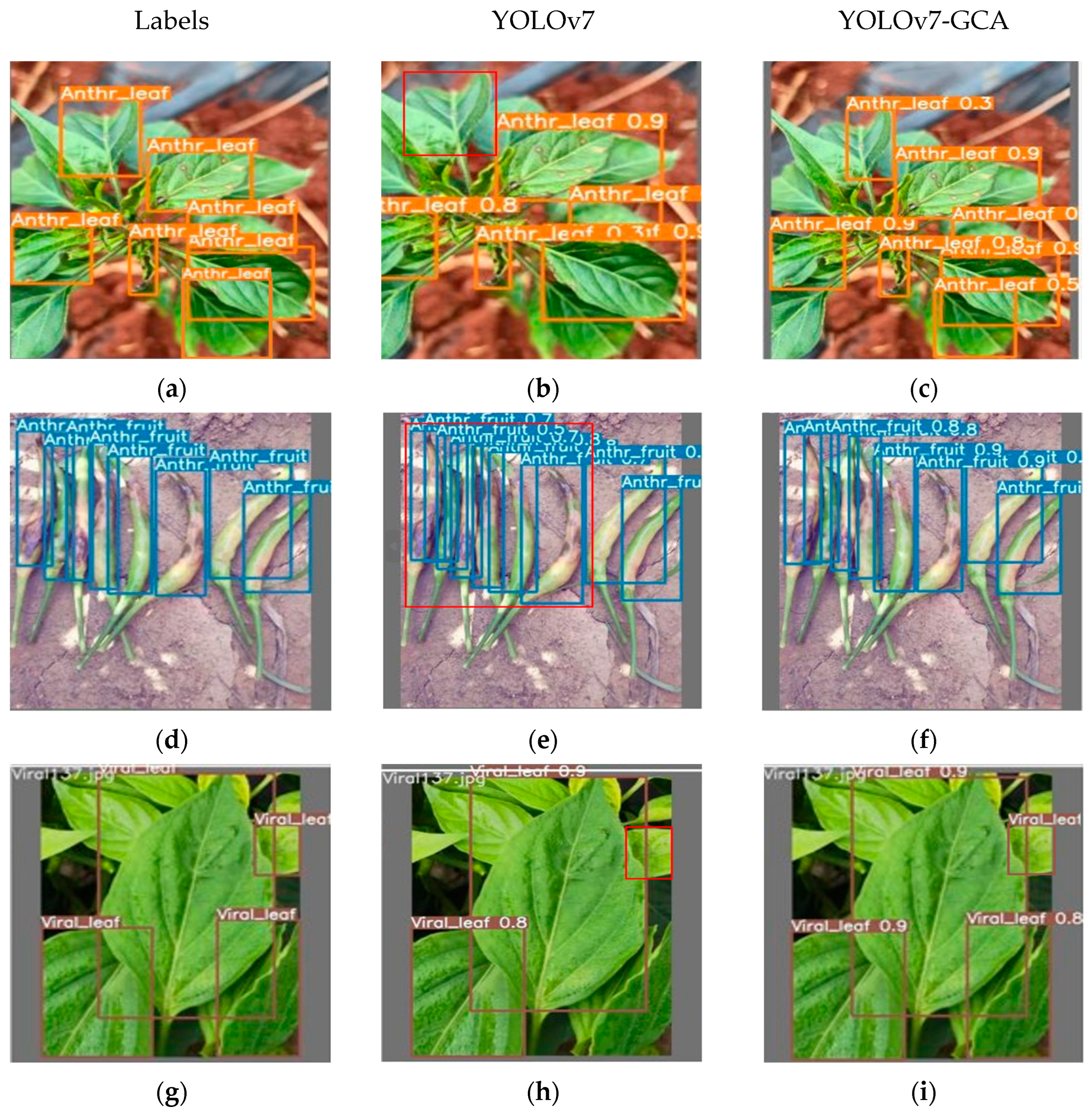
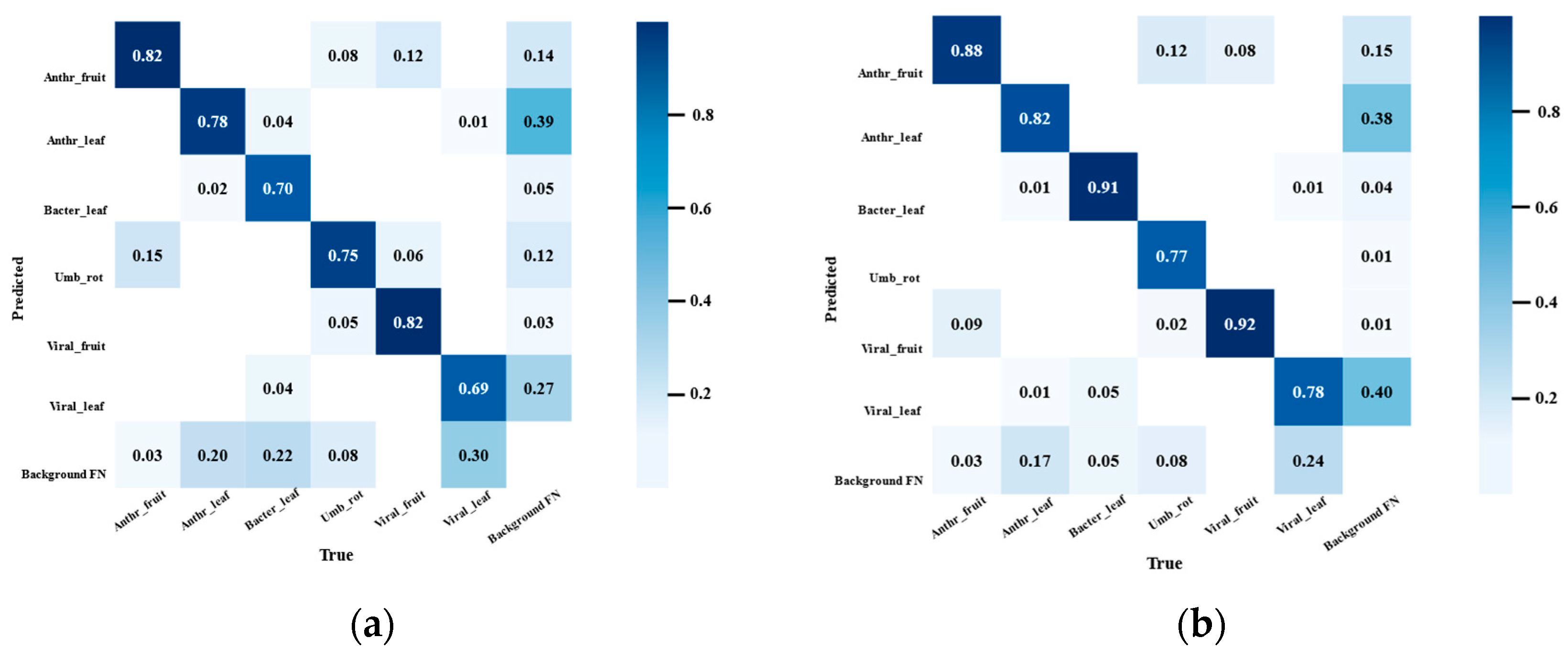
3. Results and Discussion

3.1. Model Training Results

The YOLOv7 model achieves the best accuracy within 150 epochs when using the pre-trained weights. This study trains the proposed improved model for 150 epochs for ablation experiments and compares it with the original YOLOv7 model. Figure 9 shows the training results of the YOLOv7-GCA model.

Figure 9 displays the mean loss function change curves for the YOLOv7-GCA model on the training and validation sets, as well as the PR curves and the [email protected] and [email protected]:0.95 scores. The graph shows that the mean CIOU loss, object detection loss, and classification loss converge to values close to 0, indicating that the model performs well and has good representation ability.

Figure 10 shows the performance of the original YOLOv7 model and the improved YOLOv7-GCA model in the case of occlusion and small objects. The original YOLOv7 model fails to detect the objects in Figure 10b,e,h, while the improved YOLOv7-GCA model can handle the problem of small objects and occlusion under various scenarios. Although the anchor box confidence has some fluctuations, the improved model will not appear to be missing or falsely detected. Figure 10c,f,i demonstrate the good representation ability of the YOLO-GCA model on the test set. Overall, the YOLOv7-GCA model can effectively detect the pepper diseases dataset.

3.2. Ablation Experiment

This section examines the effects of three improved methods on the network model.

Table 3. Ablation experiments of modules.

Model	[email protected] (%)	Model Size (MB)	FPS (Frames/s)	P (%)	R (%)	Params (M)
YOLOv7	83.4	71.3	178	85.6	77.9	35.49
YOLOv7 + GN	82.8	58.2	213	81.3	75.6	28.83
YOLOv7 + CF	83.53	60.3	200	87.3	71.1	29.98
YOLOv7 + CBAM	83.7	71.1	198	84.5	79.6	35.38
YOLOv7 + GN + CBAM	88.6	58.5	279	90.6	77.8	28.94
YOLOv7 + GN + CF	88.2	47.1	286	91.3	76.4	23.43
YOLOv7 + CF + CBAM	90.8	60.1	271	93.5	83.3	29.87
YOLOv7-GCA	96.8	46.9	303	95.7	93.8	23.32

presents the data plotted. Eight sets of experiments were conducted, adding different modules, and compared with the original YOLOv7 model in terms of [email protected], model size, inference speed, precision, recall, and number of parameters. The YOLOv7 model with the CFNet structure is denoted as YOLOv7 + CF, the YOLOv7 model with the GhostNetV2 module as YOLOv7 + GN, and the network with the CBAM attention module as YOLOv7 + CBAM, etc.

As shown in the first four rows of Table 3, each module improves the detection speed of the acceleration model to some extent. Replacing the CFNet structure and adding the CBAM attention module to YOLOv7 slightly increase the detection accuracy of the network, with mAP values 0.13% and 0.3% higher than the original YOLOv7 model, respectively. However, the CFNet structure does not significantly improve the recall index. Moreover, we find that the CBAM module can effectively increase the recall rate of YOLOv7 to 79.6%, which is 1.7% higher than the original version, without increasing the number of parameters. The introduction of the GhostNetV2 module or CFNet network can maintain or improve the accuracy of the model while greatly reducing the complexity and inference time, achieving results of 28.83 M and 213 frames/s and 29.98 M and 200 frames/s, respectively. In addition, the pairwise combination of modules shows that the combination of the CF + CBAM modules achieves the highest accuracy improvement, with a mAP score of 90.8% and a detection speed of 271 frames/s, which is a good performance combination. The combination of GN + CF modules can significantly accelerate the model inference speed to 286 frames/s, and the minimum parameter of the model is 23.43 m. However, introducing the CBAM module on this basis will increase the number of parameters, resulting in a slower detection speed of 7 frames/s, and the final result is 279 frames/s. Nevertheless, we believe that the combination of the three modules is a good match. Due to the GhostNet module and the CFNet module, they provide the model with accelerated inference and lightweight deployment. The attention mechanism of the CBAM module on space and channel can improve the network’s sensitivity and responsiveness to objects, thus qualitatively improving the model’s accuracy. Although our method sacrifices a very small fraction of the inference time, it brings about a significant improvement in accuracy, which is a valuable trade-off. In general, the improved model has been greatly enhanced in accuracy, number of parameters, and detection speed, and it is of great significance for the rapid and non-destructive detection of pepper diseases.

This paper evaluates the effectiveness and superiority of the YOLOv7-GCA method for pepper diseases detection. It uses the mAP and loss functions as evaluation metrics and plots the corresponding curves. The mAP is the mean accuracy (AP) of the pepper diseases detector when the IoU threshold is 0.5. IoU is the intersection over the union between two bounding boxes, which indicates the accuracy of the detector based on the object position and shape. As the IoU threshold increases, the AP value decreases, so mAP is a reliable measure of the detector’s performance at higher standards. The loss function is the optimization objective in the observation model’s training process, which indicates whether the model is overfitted or underfitted. Generally, the model is overfitting when the training loss is low and the validation loss is high; the model is underfitting when both the training and validation losses are high.

The ablation experiments used mAP as the metric and plotted the line and loss function graphs. Figure 11a shows eight curves of different colors, indicating that the GhostNetV2 module affects the model’s convergence. The mAP curves of YOLOv7 + GN, YOLOv7 + GN + CF, and YOLOv7 + GN + CBAM start to converge at around 140 epochs, while the other curves without the GhostNetV2 module converge at around 80 epochs. This implies that the GhostNetV2 module increases the model’s training difficulty by reducing the number of parameters and requiring more iterations to reach a steady state. However, the mAP of the improved YOLOv7-GCA model converges at 80 epochs, and the mAP of the YOLOv7 model converges at 82 epochs. Despite the large fluctuation in the YOLOv7 model during early training, the mAP convergence rates are similar. This suggests that the YOLOv7-GCA model’s convergence rate is not affected by the mAP enhancement. The CBAM attention mechanism and the CFNet structure jointly enhance the model’s learning ability, enable the DFC long-distance attention mechanism in the GhostNetV2 module to function, eliminate the interference of useless features, and accelerate convergence. This indicates that the YOLOv7-GCA method fully utilizes the three modules to achieve high accuracy and stability in pepper diseases detection without affecting the convergence rate.

The loss function graph in Figure 11b shows eight curves that converge at around 150 epochs. The curves of the original YOLOv7 model and the YOLOv7-GCA model are almost identical, stabilizing at 0.038 and 0.036, respectively. This indicates that the YOLOv7-GCA method can improve the detection accuracy significantly without changing the loss function level of the original method, demonstrating the superiority of this improved method for pepper diseases detection.

Figure 12 shows the predictions of the original YOLOv7 model and the improved YOLOv7-GCA model under six categories. It can be seen that the accuracy of detection for Anthr_fruit, Anthr_leaf, Bacter_leaf, Umb_rot, Viral_fruit, and Viral_leaf has improved, which verifies the feasibility and superiority of the improved model.

Overall, our method enables the YOLOv7 model to significantly improve accuracy while greatly accelerating detection and reducing computational parameters, which meets the disease monitoring requirements for agricultural production, which is a valuable improvement.

3.3. Comparison of Different Network Models

This study compares the effectiveness of the YOLOv7-GCA algorithm model with the mainstream models Faster R-CNN, SSD, YOLOv3, YOLOv5s, YOLOv8n, and the original YOLOv7 model using the same pepper diseases dataset. The specific mAP, model size, precision, recall, FPS, and FLOPs are shown in

Table 4. Comparison of seven detection models.

Model	Backbone Network	[email protected] (%)	FPS (Frames/s)	P (%)	R (%)	Params (MB)	FLOPs (G)
Faster R-CNN	ResNet-50	80.5	20	76.4	87.1	157.22	366.72
SSD	VGG16	71.2	36	72.3	65.5	24.55	270.15
YOLOv3	CSPDarknet53	77.8	53	78.3	73.5	58.64	155.15
YOLOv5s	CSPDarknet53	82.8	156	81.6	79.8	9.23	18.13
YOLOv8n	SPPCSPResNet52	84.1	183	84.7	78.1	6.31	9.55
YOLOv7	SPPCSPCDarkNet50	83.4	178	85.6	77.9	35.49	103.12
YOLOv7-GCA	SPPCSPCDarkNet58	96.8	303	95.7	93.8	23.32	65.63

. The YOLOv7-GCA model outperforms the other models in the main performance metric. The mAP of YOLOv7-GCA is 96.8%, which is much higher than the original YOLOv7 model (at 83.4%), YOLOv8n (at 86.7%), YOLOv5s (at 82.8%), YOLOv3 (at 77.8%), Faster R-CNN (at 80.5%), and SSD (at 71.2%). The precision and recall rates of the YOLOv7-GCA model were 95.7% and 93.8%, respectively, which are also higher than the other models. The combination of

GhostNetV2, CFNet, and CBAM modules optimize the original YOLOv7 model and accelerate the speed while maintaining the high mAP. The model size and FLOPs of the YOLOv7-GCA model are larger than the two lightweight models of YOLOv8n and YOLOv5s but smaller than the other networks. The average detection speed of YOLOv7-GCA in the test set is 303 frames/s, which is faster than YOLOv8n and YOLOv5. In conclusion, compared with other models, the YOLOv7-GCA model can have better detection performance and differentiation ability and can better handle the occlusion between peppers and the identification of different disease spots in each background. Therefore, when identifying pepper diseases in a complex environment, it has a lightweight and rapid detection speed, which meets the real-time needs of the agricultural field.

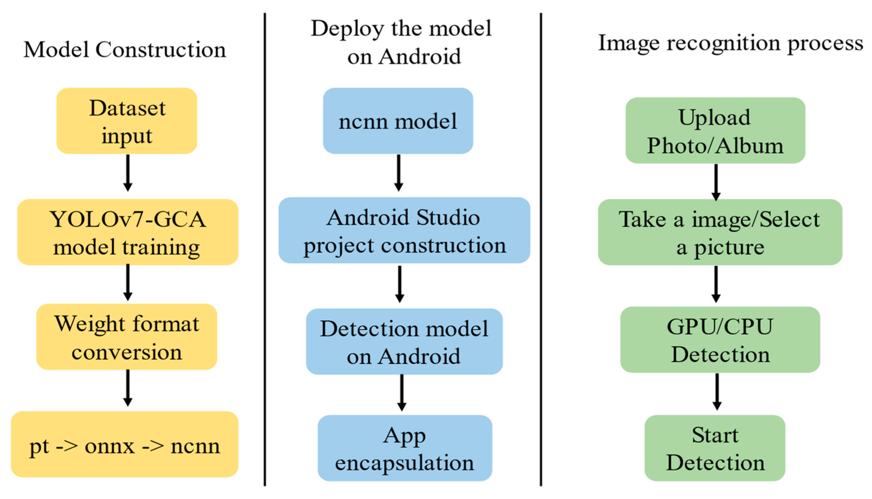
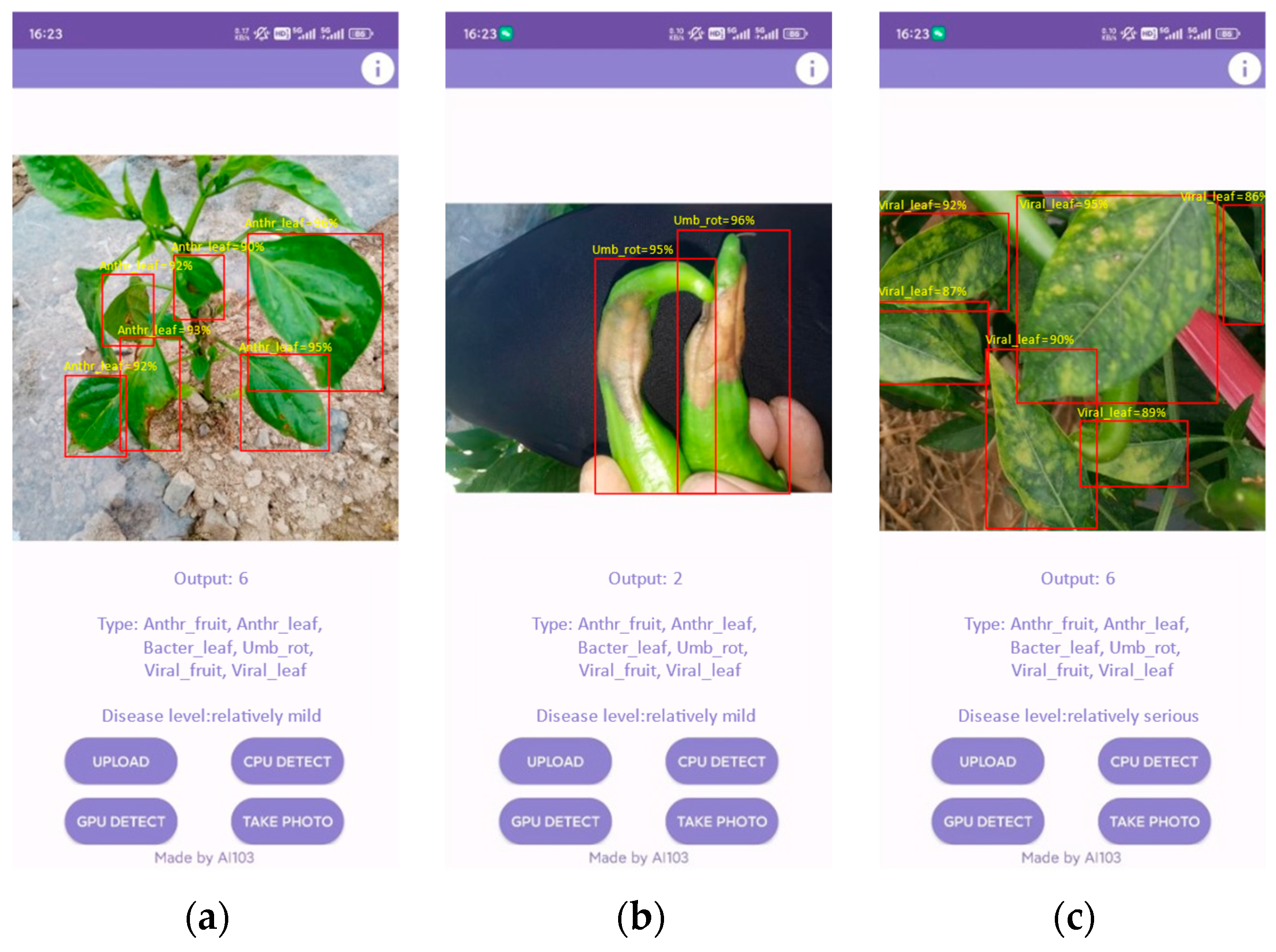
3.4. Android Deployment Testing

Deep learning models usually save their parameters in specific formats that are not compatible with all hardware platforms. To deploy a model on an Android device, the parameters need to be exported and converted to a suitable format. Figure 13 illustrates the deployment process of the pepper disease identification model on Android devices. The Ncnn Convolutional Neural Network (NCNN) is a high-performance neural network inference framework for mobile devices that supports multiple deep learning frameworks. It provides software development kits for Android and iOS, which can easily run various deep learning models on mobile devices. First, the PTH model files trained by PyTorch are converted to Open Neural Network Exchange (ONNX) model files, and then the universal properties of ONNX are used to generate the BIN and PARAM model files that the NCNN library can load. Then, the model is verified and tested. Finally, according to the design requirements of the application, an Android project is created to deploy the YOLOv7-GCA model on the phone for accuracy testing. The main functions of the pepper diseases identification app include image acquisition, automatic image saving, CPU-based pepper disease detection, GPU-based pepper disease detection, and disease grade evaluation of the detection results. Users can obtain the pepper images through the image acquisition module or use their own images from the album.

The pepper disease detection module analyzes the type, number, and severity of the diseases affecting the target pepper and outputs the number of different pepper diseases in the target image. GPU detection has the advantage of using the parallel computing power and high memory bandwidth of the GPU to speed up the inference process of the model and improve detection accuracy and efficiency. However, the model’s compatibility and stability may be affected by the diversity and performance of the mobile phone GPUs on the market. CPU detection has the advantage of being able to run on any phone without considering the GPU hardware configuration, which improves the model’s versatility and portability. Figure 14 shows the results of the pepper disease CPU-based detection on the Xiaomi13 mobile phone.

3.5. Sensitivity Analysis

Our model, YOLOv7-GCA, is based on the improvement of the YOLOv7 model, which introduces three key improvement points, namely GhostNetV2, CFNet, and CBAM. These improvement points all bring some advantages to the model but also make the performance of the model affected by some parameters. To evaluate the impact of these parameters, we selected the following three key parameters as objects for sensitivity analysis: namely, learning rate, batch size, and optimizer parameters. Learning rate is the parameter controlling the learning speed of the model, which determines the amplitude of the model updating the weights in each iteration, which affects the convergence rate and accuracy of the model. Batch size is the parameter controlling the amount of data the model processes each time, which determines the computation and memory footprint of the model in each iteration, which affects the training speed and stability of the model. The optimizer parameter is the parameter that controls the model optimization algorithm, which determines the momentum, decay, adaptation, and other factors of the model in the optimization process, which affect the convergence and robustness of the model.

The performance of the YOLOv7-GCA model varies under different parameter values, but the magnitude and direction of the change are different. We found that the learning rate has the greatest influence on the model performance. In cases where the learning rate is too large or too small, the loss function and accuracy will decrease, while when the learning rate is moderate, the loss function and accuracy of the model will reach their best, 0.03635 and 96.8%, respectively. Batch size has little influence on the performance of the model. When the batch size increases, the loss function and accuracy of the model will decrease slightly, while the speed of the model will increase slightly. The optimizer parameters also have less influence on the performance of the model, and the different optimizer parameters have no obvious differences in the loss function, accuracy, or speed of the model.

Through the sensitivity analysis in

Table 5. Sensitivity analysis.

Index	Number	Loss Function	[email protected] (%)	FPS (Frames/s)
Learning Rate	0.001	0.03705	95.5	301
Learning Rate	0.01	0.03635	96.8	303
Learning Rate	0.1	0.04175	93.4	305
Batch Size	16	0.03635	96.8	303
Batch Size	32	0.03685	96.4	313
Batch Size	64	0.03715	96.1	323
Optimization Function	Adam	0.03675	96.2	303
Optimization Function	SGD	0.03635	96.8	303
Optimization Function	RMSprop	0.03655	96.3	303

, we obtained the following conclusions and implications: First, our model, YOLOv7-GCA, was able to achieve better performance under different parameter values, demonstrating the robustness and adaptability of the model. Second, our model YOLOv7-GCA performs best at the learning rate of 0.01, the batch size of 16, and the optimizer parameter of SGD, demonstrating that these parameters are the optimal parameter settings for the model. Finally, the advantage of our model YOLOv7-GCA over other models is that it achieves a balanced performance in speed, model size, and accuracy, illustrating the effectiveness and superiority of the model.

4. Conclusions

In this paper, we propose a novel model, YOLOv7-GCA, for pepper disease detection in complex environments. It introduces three main improvements to the model. The first is using lightweight GhostNetV2 as a backbone network to eliminate redundant information and enhance feature extraction efficiency. The second one is adding CFNet to achieve deeper and more effective multi-scale feature fusion and improve the performance of intensive tasks. The third one is reorganizing and optimizing the feature extraction and detection components of the YOLOv7 backbone network, neck, and head using the CBAM attention module that considers channels and space. The YOLOv7-GCA model compares six object detectors on test datasets and performs well on multiple indicators. Its mAP is 96.8%, which is 12.7%, 13.4%, 14.0%, 19.0%, 25.6%, and 16.3% higher than the YOLOv8n, YOLOv7, YOLOv5s, YOLOv3, SSD, and Faster R-CNN models, respectively. Regarding detection speed and lightweight, the YOLOv7-GCA model’s average detection speed is 303 frames/s, which is faster than the original YOLOv7 model’s 178 frames/s. The number of parameters is reduced by nearly 34%, and the model size is compressed to 46.9 MB. This demonstrates that the YOLOv7-GCA model can achieve lightweight deployment and high detection accuracy and can be applied to pepper disease detection in real-world environments. For future work, we plan to further improve the other module structures of the model, such as context learning, utilize the information related to the object in the image, and increase the model’s adaptability to different scenes. We hope that our study will provide some technical assistance for future pepper disease detection research and help farmers identify and manage the pepper disease situation effectively.

References

1. Karim, K.M.R.; Rafii, M.Y.; Misran, A.B.; Ismail, M.F.B.; Harun, A.R.; Khan, M.M.H.; Chowdhury, M.F.N. Current and Prospective Strategies in the Varietal Improvement of Chilli (Capsicum annuum L.) Specially Heterosis Breeding. Agronomy 2021, 11, 2217. [Google Scholar] [CrossRef]
2. Olatunji, T.L.; Afolayan, A.J. The suitability of chili pepper (Capsicum annuum L.) for alleviating human micronutrient dietary deficiencies: A review. Food Sci. Nutr. 2018, 6, 2239–2251. [Google Scholar] [CrossRef] [PubMed]
3. Ahmed, H.F.A.; Seleiman, M.F.; Mohamed, I.A.A.; Taha, R.S.; Wasonga, D.O.; Battaglia, M.L. Activity of Essential Oils and Plant Extracts as Biofungicides for Suppression of Soil-Borne Fungi Associated with Root Rot and Wilt of Marigold (Calendula officinalis L.). Horticulturae 2023, 9, 222. [Google Scholar] [CrossRef]
4. Ahmed, H.F.A.; Elnaggar, S.; Abdel-Wahed, G.A.; Taha, R.S.; Ahmad, A.; Al-Selwey, W.A.; Ahmed, H.M.H.; Khan, N.; Seleiman, M.F. Induction of Systemic Resistance in Hibiscus sabdariffa Linn. to Control Root Rot and Wilt Diseases Using Biotic and Abiotic Inducers. Biology 2023, 12, 789. [Google Scholar] [CrossRef] [PubMed]
5. Saleem, M.H.; Potgieter, J.; Arif, K.M. Automation in Agriculture by Machine and Deep Learning Techniques: A Review of Recent Developments. Precis. Agric. 2021, 22, 2053–2091. [Google Scholar] [CrossRef]
6. Zhou, H.; Wang, X.; Au, W.; Kang, H.; Chen, C. Intelligent robots for fruit harvesting: Recent developments and future challenges. Precis. Agric. 2022, 23, 1856–1907. [Google Scholar] [CrossRef]
7. Li, L.; Zhang, S.; Wang, B. Plant Disease Detection and Classification by Deep Learning—A Review. IEEE Access 2021, 9, 56683–56698. [Google Scholar] [CrossRef]
8. Zhang, C.; Zhang, S.; Yang, J.; Shi, Y.; Chen, J. Apple leaf disease identification using genetic algorithm and correlation based feature selection method. Int. J. Agric. Biol. Eng. 2017, 10, 74–83. [Google Scholar]
9. Chakraborty, S.; Paul, S.; Rahat-uz-Zaman, M. Prediction of Apple Leaf Diseases Using Multiclass Support Vector Machine. In Proceedings of the 2021 2nd International Conference on Robotics, Electrical and Signal Processing Techniques (ICREST), Dhaka, Bangladesh, 5–7 January 2021. [Google Scholar]
10. Zhang, S.; Wu, X.; You, Z.; Zhang, L. Leaf image based cucumber disease recognition using sparse representation classification. Comput. Electron. Agric. 2017, 134, 135–141. [Google Scholar] [CrossRef]
11. Singh, A.K.; Sreenivasu, S.V.N.; Mahalaxmi, U.S.B.K.; Sharma, H.; Patil, D.D.; Asenso, E. Hybrid Feature-Based Disease Detection in Plant Leaf Using Convolutional Neural Network, Bayesian Optimized SVM, and Random Forest Classifier. J. Food Qual. 2022, 2022, 2845320. [Google Scholar] [CrossRef]
12. Loti, N.N.A.; Noor, M.R.M.; Chang, S.-W. Integrated Analysis of Machine Learning and Deep Learning in Chili Pest and Disease Identification. J. Sci. Food Agric. 2020, 101, 3582–3594. [Google Scholar] [CrossRef]
13. Neupane, K.; Baysal-Gurel, F. Automatic Identification and Monitoring of Plant Diseases Using Unmanned Aerial Vehicles: A Review. Remote Sens. 2021, 13, 3841. [Google Scholar] [CrossRef]
14. Jiang, P.; Ergu, D.; Liu, F.; Cai, Y.; Ma, B. A Review of Yolo Algorithm Developments. Procedia Comput. Sci. 2022, 199, 1066–1073. [Google Scholar] [CrossRef]
15. Zhang, K.; Wu, Q.; Chen, Y. Detecting soybean leaf disease from synthetic image using multi-feature fusion faster R-CNN. Comput. Electron. Agric. 2021, 183, 106064. [Google Scholar] [CrossRef]
16. Sun, H.; Xu, H.; Liu, B.; He, D.; He, J.; Zhang, H.; Geng, N. MEAN-SSD: A novel real-time detector for apple leaf diseases using improved light-weight convolutional neural networks. Comput. Electron. Agric. 2021, 189, 106379. [Google Scholar] [CrossRef]
17. Bao, W.; Fan, T.; Hu, G.; Liang, D.; Li, H. Detection and identification of tea leaf diseases based on AX-RetinaNet. Sci. Rep. 2022, 12, 2183. [Google Scholar] [CrossRef] [PubMed]
18. Diwan, T.; Anirudh, G.; Tembhurne, J.V. Object detection using YOLO: Challenges, architectural successors, datasets and applications. Multimed. Tools Appl. 2023, 82, 9243–9275. [Google Scholar] [CrossRef]
19. Lippi, M.; Bonucci, N.; Carpio, R.F.; Contarini, M.; Speranza, S.; Gasparri, A. A YOLO-Based Pest Detection System for Precision Agriculture. In Proceedings of the 2021 29th Mediterranean Conference on Control and Automation (MED), Puglia, Italy, 22–25 June 2021. [Google Scholar]
20. Liu, J.; Wang, X. Plant diseases and pests detection based on deep learning: A review. Plant Methods 2021, 17, 22. [Google Scholar] [CrossRef]
21. Liu, J.; Wang, X. Tomato Diseases and Pests Detection Based on Improved Yolo V3 Convolutional Neural Network. Front. Plant Sci. 2020, 11, 521544. [Google Scholar] [CrossRef]
22. Wang, X.; Liu, J. Tomato Anomalies Detection in Greenhouse Scenarios Based on YOLO-Dense. Front. Plant Sci. 2021, 12, 634103. [Google Scholar] [CrossRef]
23. Li, D.; Ahmed, F.; Wu, N.; Sethi, A.I. YOLO-JD: A Deep Learning Network for Jute Diseases and Pests Detection from Images. Plants 2022, 11, 937. [Google Scholar] [CrossRef]
24. Fang, W.; Guan, F.; Yu, H.; Bi, C.; Guo, Y.; Cui, Y.; Su, L.; Zhang, Z.; Xie, J. Identification of wormholes in soybean leaves based on multi-feature structure and attention mechanism. J. Plant Dis. Prot. 2022, 130, 401–412. [Google Scholar] [CrossRef]
25. Xue, Z.; Xu, R.; Bai, D.; Lin, H. YOLO-Tea: A Tea Disease Detection Model Improved by YOLOv5. Forests 2023, 14, 415. [Google Scholar] [CrossRef]
26. Xu, W.; Wang, R. ALAD-YOLO: An lightweight and accurate detector for apple leaf diseases. Front. Plant Sci. 2023, 14, 1204569. [Google Scholar] [CrossRef] [PubMed]
27. Yang, S.; Xing, Z.; Wang, H.; Dong, X.; Gao, X.; Liu, Z.; Zhang, X.; Li, S.; Zhao, Y. Maize-YOLO: A New High-Precision and Real-Time Method for Maize Pest Detection. Insects 2023, 14, 278. [Google Scholar] [CrossRef] [PubMed]
28. Jia, L.; Wang, T.; Chen, Y.; Zang, Y.; Li, X.; Shi, H.; Gao, L. MobileNet-CA-YOLO: An Improved YOLOv7 Based on the MobileNetV3 and Attention Mechanism for Rice Pests and Diseases Detection. Agriculture 2023, 13, 1285. [Google Scholar] [CrossRef]
29. Tang, Y.; Han, K.; Guo, J.; Xu, C.; Xu, C.; Wang, Y. GhostNetv2: Enhance cheap operation with long-range attention. Adv. Neural Inf. Process. Syst. 2022, 35, 9969–9982. [Google Scholar]
30. Zhang, G.; Li, Z.; Li, J.; Hu, X. Cfnet: Cascade fusion network for dense prediction. arXiv 2023, arXiv:2302.06052. [Google Scholar]
31. Woo, S.; Park, J.; Lee, J.-Y.; Kweon, I.S. CBAM: Convolutional Block Attention Module. In Lecture Notes in Computer Science; Springer International Publishing: Cham, Germany, 2018. [Google Scholar]
32. Lin, T.; Maire, M.; Belongie, S.; Hays, J.; Perona, P.; Ramanan, D.; Dollár, P.; Zitnick, C. Microsoft coco: Common objects in context. In Proceedings of the European Conference on Computer Vision, Zurich, Switzerland, 6–12 September 2014; pp. 740–755. [Google Scholar]
33. Ying, Z.; Li, G.; Ren, Y.; Wang, R.; Wang, W. A New Image Contrast Enhancement Algorithm Using Exposure Fusion Framework. In Lecture Notes in Computer Science; Springer International Publishing: Cham, Germany, 2017; pp. 36–46. [Google Scholar]
34. DeVries, T.; Taylor, G.W. Improved Regularization of Convolutional Neural Networks with Cutout. arXiv 2017, arXiv:1708.04552. [Google Scholar]
35. Shorten, C.; Khoshgoftaar, T.M. A survey on Image Data Augmentation for Deep Learning. J. Big Data 2019, 6, 60. [Google Scholar] [CrossRef]
36. Zhong, Z.; Zheng, L.; Kang, G.; Li, S.; Yang, Y. Random Erasing Data Augmentation. In Proceedings of the AAAI Conference on Artificial Intelligence, New York, NY, USA, 7–12 February 2020; Volume 34, pp. 13001–13008. [Google Scholar] [CrossRef]
37. Simonyan, K.; Zisserman, A. Very Deep Convolutional Networks for Large-Scale Image Recognition. arXiv 2015, arXiv:1409.1556. [Google Scholar]
38. Takahashi, R.; Matsubara, T.; Uehara, K. Data Augmentation Using Random Image Cropping and Patching for Deep CNNs. IEEE Trans. Circuits Syst. Video Technol. 2020, 30, 2917–2931. [Google Scholar] [CrossRef]
39. Bochkovskiy, A.; Wang, C.-Y.; Liao, H.-Y.M. YOLOv4: Optimal Speed and Accuracy of Object Detection. arXiv 2020, arXiv:2004.10934. [Google Scholar]
40. WongKinYiu. YOLOv7.Git Code. 2022. Available online: https://github.com/WongKinYiu/yolov7 (accessed on 20 November 2022).
41. Wang, C.-Y.; Bochkovskiy, A.; Liao, H.-Y.M. YOLOv7: Trainable Bag-of-Freebies Sets New State-of-the-Art for Real-Time Object Detectors. In Proceedings of the 2023 IEEE/CVF Conference on Computer Vision and Pattern Recognition (CVPR), Vancouver, BC, Canada, 17–24 June 2023. [Google Scholar]
42. Redmon, J.; Divvala, S.; Girshick, R.; Farhadi, A. You Only Look Once: Unified, Real-Time Object Detection. In Proceedings of the 2016 IEEE Conference on Computer Vision and Pattern Recognition (CVPR), Las Vegas, NV, USA, 27–30 June 2016. [Google Scholar]
43. Ding, X.; Zhang, X.; Ma, N.; Han, J.; Ding, G.; Sun, J. RepVGG: Making VGG-style ConvNets Great Again. In Proceedings of the 2021 IEEE/CVF Conference on Computer Vision and Pattern Recognition (CVPR), Nashville, TN, USA, 20–25 June 2021. [Google Scholar]
44. Wang, C.-Y.; Bochkovskiy, A.; Liao, H.-Y.M. Scaled-YOLOv4: Scaling Cross Stage Partial Network. In Proceedings of the 2021 IEEE/CVF Conference on Computer Vision and Pattern Recognition (CVPR), Nashville, TN, USA, 20–25 June 2021. [Google Scholar]
45. Lv, Y.; Ai, Z.; Chen, M.; Gong, X.; Wang, Y.; Lu, Z. High-Resolution Drone Detection Based on Background Difference and SAG-YOLOv5s. Sensors 2022, 22, 5825. [Google Scholar] [CrossRef]
46. Hu, J.; Shen, L.; Sun, G. Squeeze-and-Excitation Networks. In Proceedings of the 2018 IEEE/CVF Conference on Computer Vision and Pattern Recognition, Salt Lake City, UT, USA, 18–22 June 2018. [Google Scholar]
47. Howard, A.G.; Zhu, M.; Chen, B.; Kalenichenko, D.; Wang, W.; Weyand, T.; Andreetto, M.; Adam, H. MobileNets: Efficient Convolutional Neural Networks for Mobile Vision Applications. arXiv 2017, arXiv:1704.04861. [Google Scholar]
48. Han, K.; Wang, Y.; Tian, Q.; Guo, J.; Xu, C.; Xu, C. GhostNet: More Features From Cheap Operations. In Proceedings of the 2020 IEEE/CVF Conference on Computer Vision and Pattern Recognition (CVPR), Seattle, WA, USA, 13–19 June 2020. [Google Scholar]
49. Zheng, Z.; Wang, P.; Liu, W.; Li, J.; Ye, R.; Ren, D. Distance-IoU Loss: Faster and Better Learning for Bounding Box Regression. In Proceedings of the AAAI Conference on Artificial Intelligence, New York, NY, USA, 7–12 February 2020; Volume 34, pp. 12993–13000. [Google Scholar] [CrossRef]
Figure 1. Example diagram of data augmentation: (a) Original image; (b) Contrast data augmentation; (c) Cutout data augmentation; (d) Rotation; (e) Kernel Filters; (f) Add salt-and-pepper noise noise; (g) Scaling; (h) Random cropping; (i) Mosaic data augmentation.
Agronomy 14 00618 g001
Figure 2. The network structure of the original YOLOv7.
Agronomy 14 00618 g002
Figure 3. DFC mechanism and GhostNetV2 module. Mul is feature map multiplication. Add is feature map addition.
Agronomy 14 00618 g003
Figure 4. GhostNetV2 information aggregation process diagram.
Agronomy 14 00618 g004
Figure 5. CBAM algorithm implementation flowchart.
Agronomy 14 00618 g005
Figure 6. The network structure of CFNet.
Agronomy 14 00618 g006
Figure 7. Illustration of the CIoU loss formula.
Agronomy 14 00618 g007
Figure 8. YOLOv7-GCA Network architecture.
Agronomy 14 00618 g008
Figure 9. Results of the PR plots in the YOLOv7 (a) and YOLOv7-GCA (b) models.
Agronomy 14 00618 g009
Figure 10. Recognition effect analysis: (a,d,g) are the labeled results; (b,e,h) are the YOLOv7 detection results; (c,f,i) are the YOLOv7-GCA detection results.
Agronomy 14 00618 g010
Figure 11. The mAP (a) and training loss (b) of the ablation experiments.
Agronomy 14 00618 g011
Figure 12. Confusion matrix of YOLOv7 (a) and YOLOv7-GCA (b) to identify results.
Agronomy 14 00618 g012
Figure 13. Flowchart of deployment process on Android terminal.
Agronomy 14 00618 g013
Figure 14. Effective picture for pepper disease detection: (a) anthracnose; (b) umbilical rot diseases; (c) viral diseases.
Agronomy 14 00618 g014