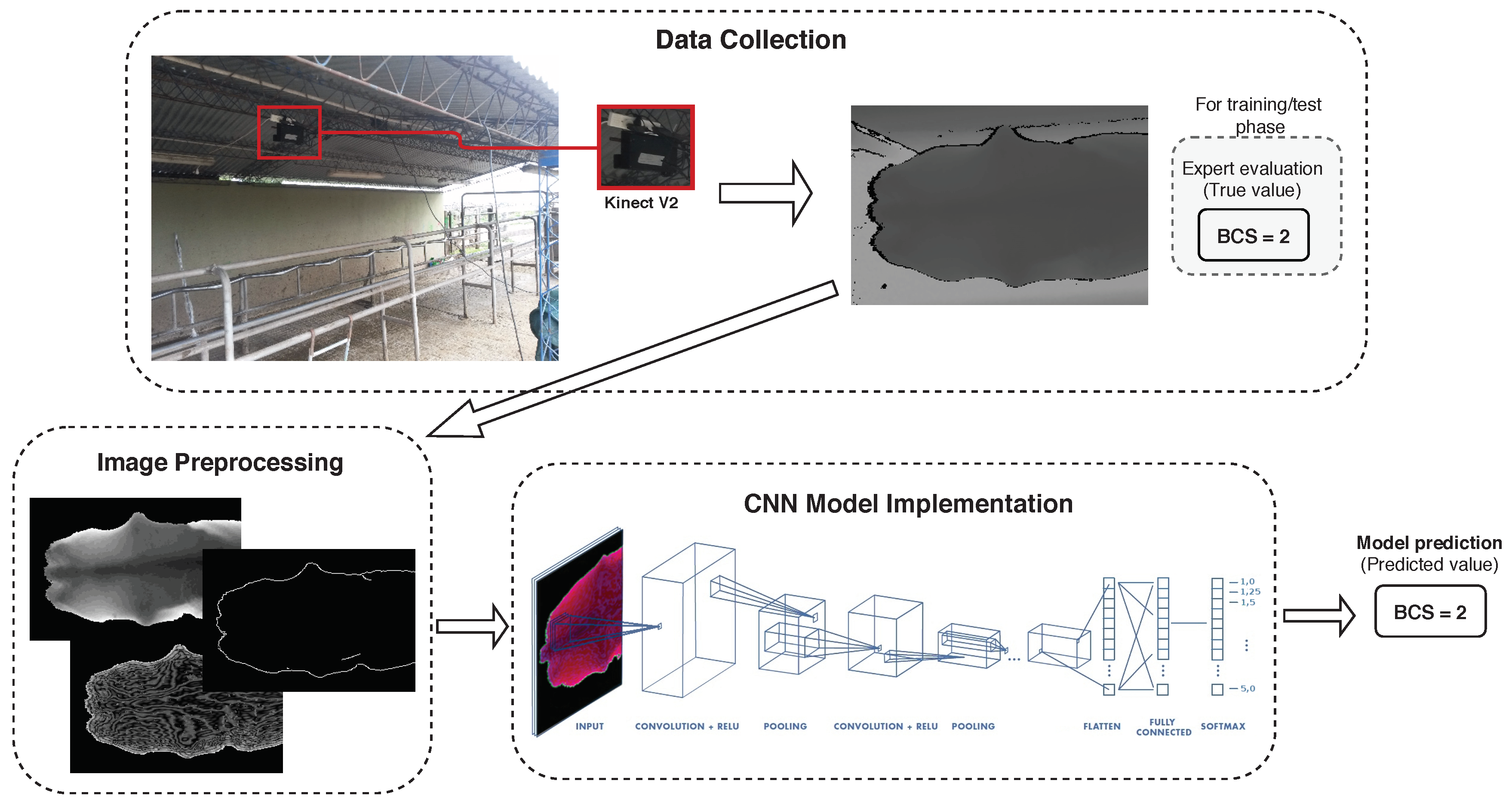
Article

Estimating Body Condition Score in Dairy Cows From Depth Images Using Convolutional Neural Networks, Transfer Learning and Model Ensembling Techniques

1
CIVETAN (Facultad de Ciencias Veterinarias—UNCPBA, CICPBA and CONICET), UNICEN University, Tandil B7001BBO, Argentina
2
D-TEC—Agencia Nacional de Promoción Científica y Tecnológica (ANPCyT), CABA C1425FQD, Argentina
3
ISISTAN-CONICET, UNICEN University, Tandil B7001BBO, Argentina
4
Facultad de Ciencias Veterinarias, UNICEN University, Tandil B7001BBO, Argentina
*
Author to whom correspondence should be addressed.
Current address: ISISTAN-UNICEN-CONICET, UNICEN University, Campus Universitario, Tandil B7001BBO, Buenos Aires, Argentina.
Submission received: 28 December 2018 / Revised: 5 February 2019 / Accepted: 12 February 2019 / Published: 16 February 2019
(This article belongs to the Special Issue Deep Learning Techniques for Agronomy Applications)

Abstract

:
BCS (Body Condition Score) is a method to estimate body fat reserves and accumulated energy balance of cows, placing estimations (or BCS values) in a scale of 1 to 5. Periodically rating BCS of dairy cows is very important since BCS values are associated with milk production, reproduction, and health of cows. However, in practice, obtaining BCS values is a time-consuming and subjective task performed visually by expert scorers. There have been several efforts to automate BCS of dairy cows by using image analysis and machine learning techniques. In a previous work, an automatic system to estimate BCS values was proposed, which is based on Convolutional Neural Networks (CNNs). In this paper we significantly extend the techniques exploited by that system via using transfer learning and ensemble modeling techniques to further improve BCS estimation accuracy. The improved system has achieved good estimations results in comparison with the base system. Overall accuracy of BCS estimations within 0.25 units of difference from true values has increased 4% (up to 82%), while overall accuracy within 0.50 units has increased 3% (up to 97%).

1. Introduction

BCS (“Body Condition Score”) is a technique for visually estimating body fat reserves which have no direct correlation with body weight and frame size [1]. BCS is a 5-point scale system with 0.25-point intervals; in this system, cows with a score of 1 are emaciated, while cows with a score of 5 are obese [2,3]. BCS is especially important for dairy cows as it is not only a measurement of obesity degree, but also a suitable assessment of feeding management according to each stage of lactation, which heavily influences milk production, reproduction, and cow health. Despite its importance, BCS is currently a time-consuming manual task performed by expert. Furthermore, results are subjective as the experts estimate BCS scores relaying only in a naked-eye inspection and their experience.
The increasing advances in technology availability at an accessible cost, automation, and digitalization of livestock farming tasks offer multiple opportunities to aid BCS estimation. In this context, different studies have particularly focused on BCS automation using digital images [4,5,6,7,8,9,10]. In these works the traditional model of pattern/image recognition was applied, in which a by hand-designed feature extractor gathers relevant information from the input image. Then, features are used to train a classifier (or a regression model), which outputs the class (or value) corresponding to an input image.
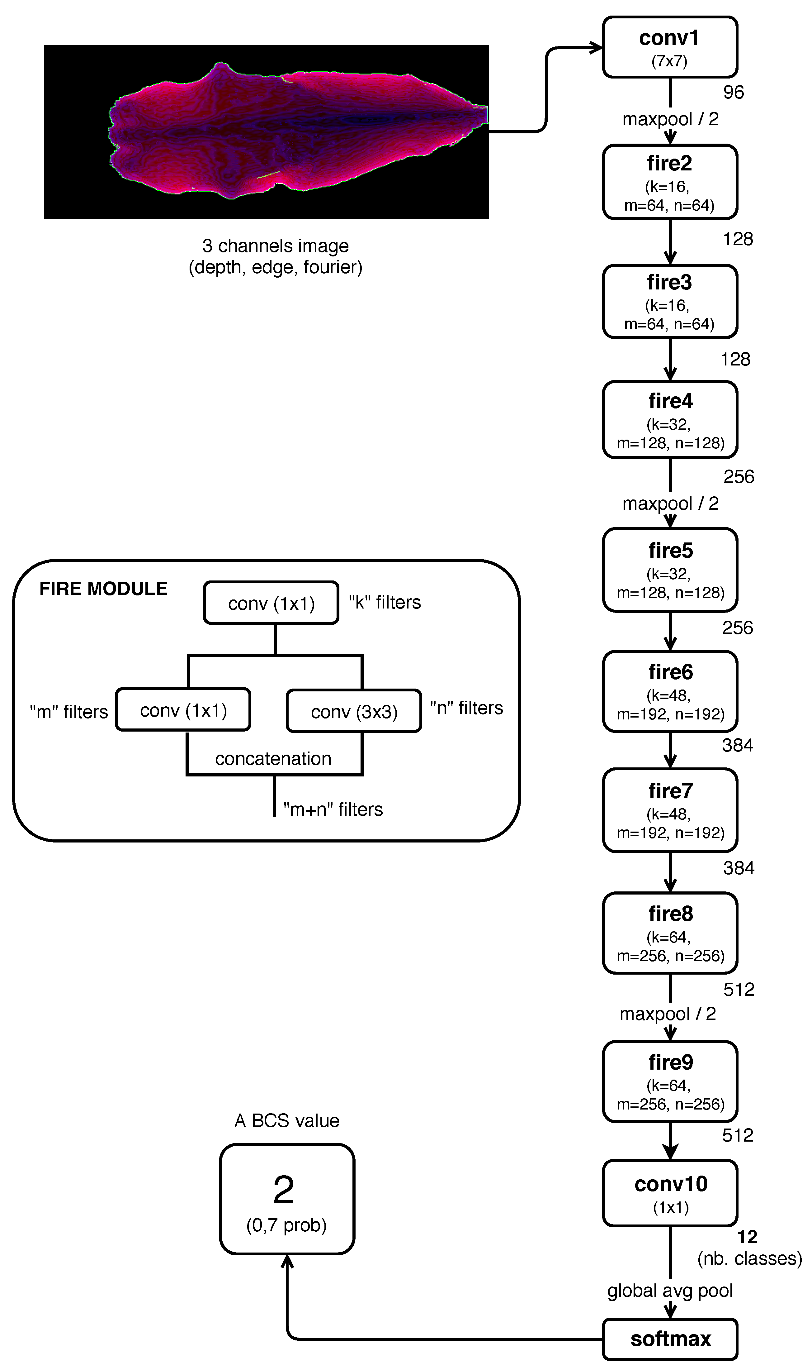
However, an alternative technique from the field of Deep Leaning, known as Convolutional Neural Network (CNN), has been found highly effective and been commonly used in computer vision and image classification [11,12,13,14,15]. A CNN is a specialized kind of neural network with a particular architecture composed of a sequence three types of layers: convolutional, pooling (or subsampling) and fully-connected. In a CNN, convolution and pooling layers play the role of feature extractor, where the weights (model coefficients or parameters) of the convolutional layer being used for feature extraction as well as the fully connected layer being used for classification are automatically determined during the training process [12]. Thus, CNNs have the advantage of locating the important features itself through training, reducing the need for by-hand feature engineering, which is a complex, time-consuming, and experts’ knowledge dependent process, whose performance could affect the overall results [16].
Although CNNs, and more generally deep learning techniques, have been successfully applied in various domains, its adoption in agriculture tasks is relatively recent. Kamilaris et al. [16] have performed a survey of 40 research works that employ deep learning techniques in the agriculture domain, among which only 3 works correspond to livestock activities. Within these, Demmers et al. [17,18] have developed first order DRNN (Differential Recurrent Neural Networks) models to control and predict growth of pigs and broiler chickens (by estimating their weight) using field sensory data and a combination of static and dynamic environmental variables. Santoni et al. [19] have built a CNN model to classify cattles into 5 different races using grayscale images.
That is why, with the objective to exploit the benefits of deep learning in the cows’ BCS estimation problem, a novel CNN-based model was proposed in a recent published work [15] to estimate BCS on cows from depth images. The development system has achieved very good results in comparison with related works, improving the classification accuracy within different error ranges (0.25, 0.50 BCS units) which are measures commonly used in literature to analyze model efficiency. However, obtaining close-to-ideal BCS estimations is still an open problem, so a detailed analysis of potential improvements could be carried out taking into account other model configurations and strategies. Particularly, two of the strategies considered in this work are transfer learning and model ensembling. Transfer learning aims to extract and transfer the knowledge from some source tasks to a target task when the latter has fewer high-quality training data [20]. The main goal of this technique is to train the lower network layers, i.e., the ones which are closest to the input, which are likely to learn general features that can be fed to classifier, usually a shallow neural network, with less variance than a full deep neural network. On the other hand, model ensembling is a machine learning technique that combines the decisions from multiple models to improve the overall performance, based on the concept that a diverse set of model are likely to make better predictions in comparison to single models like [15].
Therefore, the aim of this work is to develop alternative models employing different architecture configurations and commonly used techniques in deep learning area to study and analyze their impact and benefits when estimating BCS on cows. The next Section discusses the data used to train and test the system, explains the use of CNNs for the problem at hand, and presents our improvements to the approach first described in [15]. Section 3 analyzes the obtained results. Finally, Section 4 concludes the paper.

2. Materials and Methods

Figure 1 overviews the developed system in a recent published work [15] oriented towards estimating dairy cow BCS values from depth images. This general method was adopted in this work too, focusing on the analysis of different CNN model implementations in order to improve previous results. Section 2.1 describes the image collection process followed and the dataset used to train and validate the new proposed BCS classification models. Section 2.2 presents the techniques and considerations that were taken into account to preprocess collected images. Section 2.3 describes the CNN models analyzed in this work, considering different approaches and learning techniques. Finally, Section 2.4 presents the metrics used to evaluated models performance.

2.1. Image Collection Process and Employed Dataset

In order to train and validate proposed models, a dataset of 1661 cow images was built. A Microsoft Kinect v2 camera was used to capture the images from the top as cows voluntarily walked below it. The device was located at the exit of the milk parlor at 2.8 m above ground, and aimed downward to an area that was not exposed to direct sunlight avoiding Kinect problems under sunlight conditions (bad image quality or noise). Depth 512 × 424 images were used to train/test the analyzed approaches because they have proven to be more suitable than RGB images to depict cow body variability associated with changes in BCS [5]. During the acquisition of the cow images, an expert scorer rated the BCS of cows in situ.
The dataset was split into training and test sets. In this sense, 70% of the images (1158) were used for model development (training) and the remaining images (503) were used for model validation. Both datasets were composed of BCS values ranging from 1.75 to 4.5 preserving samples distribution of the whole dataset, i.e., images were distributed proportionally into both datasets, as Table 1 and Figure 2 show.

2.2. Images Preprocessing

First of all, a segmentation between background objects and the cow in the image was applied to filter pixels that do not belong to a cow’s body. To do this, a capture of the empty scene was set as background image and it was subtracted to cow images. Thus, only a cow’s back end that was not present in the background image were conserved. Additionally, pixels located above 1.8 m from the floor were filtered out, assuming that there are no cows taller than this value and therefore they were irrelevant. Depth values was rescaled from 0 to 255 (8 bits representation) highlighting cow’s body variability, and making them independent of animal size.
The resulted depth image was transformed to generate 2 additional channels. One of them used discrete Fourier transform to perform filtering operations to adjust the spatial frequency content of the depth image. To do that, firstly a Fourier transform was used to find the frequency domain of the depth image. Secondly, the transformed image was manipulated applying a high-pass filtering, preserving only the higher spatial frequency components. Lastly, an inverse Fourier transform was performed to produce the final filtered image for the new channel, which preserves all of the sharp crisp edges from the original depth image. The other channel was generated using the Canny algorithm [21], an edge detector method used to locate sharp intensity changes and to find object boundaries [22], which allowed for the cow’s body contour to be highlighted.

2.3. BCS Estimation Models

2.3.1. CNN Models Trained From Scratch

In the previous work [15], a CNN model based on SqueezeNet [23] architecture was implemented to estimate BCS (Figure 3), achieving very good results in comparison with related works. In that work, preprocessed images composed by the three channels presented in Section 2.2 were used as CNN input values.
However, the number of input channels taking into account was not deeply analyzed in [15]. The results published in [15] considered only a network with the three channels. Thus, in this work models composed by one (Depth) and two (Depth and Edge) input channels were also analyzed, using the same architecture model defined in [15] (Figure 3). Then, new models were identified as follow:
  • Model 1: input image composed by one channel (Depth).
  • Model 2: input image composed by two channel (Depth and Edge).
  • Model 3: input image composed by three channel (Depth, Edge, Fourier).
Other combinations of one and two input channels were not analyzed because, firstly it is important to preserve a part or a partial variation of the original data (depth data), and secondly because data corresponding to the contour of the cows (edge data) have also proven to be a determinant feature (in machine learning terms) to guide the estimation of BCS from images, as evidenced in previous works [4,6,7,8,9,24,25].

2.3.2. Transfer Learning

A common and highly effective approach to deep learning on small image datasets (datasets with 500 images per class or even less [26]) is to use a pretrained network (over thousands or millions of images), and then use part of the acquired knowledge by this network to solve a new task of interest [27]. This approach is known as transfer learning. In transfer learning, a base network is trained on a base dataset and task (usually a big one, such as the well-known ImageNet (http://image-net.org) dataset), and then the learned features are repurposed or transferred to a second target network to be trained on a target dataset and task. This process will tend to work if the features are general, meaning suitable to both base and target tasks, instead of specific to the base task. In this sense, transfer learning can be very useful to train a model on a target dataset which is significantly smaller than the base dataset, avoiding overfitting [28].
The usual transfer learning approach is to train a base network and then copy its first n layers to the first “n” layers of a target network. The remaining layers of the target network are then randomly initialized and trained toward the target task of classifying cow images by BCS. It is possible to identify two principal techniques to apply transfer learning, kwown as feature extraction and fine-tuning.
The first one consists of using the representations learned by a previous network to extract interesting features from new samples, and then run those features through a new classifier, which is trained from scratch. A CNN used for image classification comprise two parts: a series of pooling and convolution layers, and a final densely connected classifier. The first part is called the convolutional base of the model. Feature extraction (in CNN context) consists of taking the convolutional base of a previously trained network, running the new data through it, and training a new classifier on top of the output [27]. The weights of the transferred feature layers (convolutional base) are left frozen, meaning that they do not change during training on the new task [28]. It is important to reuse only the convolutional base of the pretrained model because the representations learned by this part are likely to be more generic and therefore more reusable (generic concepts which are likely to be useful regardless of the computer-vision problem at hand). In addition, it is necessary to train a new classifier because the new representations learned by this part should be specific to the set of classes on which the model was trained [27].
The second widely used technique, fine tuning, consists of unfreezing a few of the top layers of a frozen model base used for feature extraction, and jointly training both the newly added part of the model (new classifier) and these top layers. This is called fine-tuning because it slightly adjusts the more abstract representations of the model being reused, in order to make them more relevant for the problem at hand. It is important that previous to fine-tuning the top layers, the new added classifier is trained by using the feature extraction technique. If the classifier is not already trained (its weights are randomly initialized), then the error signal propagating through the network during training will be too large, and the representations previously learned by the layers being fine-tuned will be destroyed. In addition, it is not recommendable to fine-tune all layers in the convolutional base for two main reasons. One of them, because the first layers encode more generic, reusable features (edges, textures, etc.), whereas layers close to the end encode more specialized features (rounded contours, angular contours, anatomical parts of cow). In this sense, it may be more convenient to adjust more specialized features since these are the ones that must be readjusted to the new problem, i.e., differentiate changes in the BCS of the cows. The other reason, because the risk of overfitting is greater when more parameters (weights) need to be train. That is why generally it is a good strategy to fine-tune only the top two or three layers in the convolutional base [27].
In this paper, Keras API [29] was used to implement the previous described transfer learning alternatives. Keras has deep learning models implemented with pre-trained weights over the ImageNet data set, of which VGG16 [30] model was used to analyze the impact of these techniques. Keras provides support to build model architecture, load its weights, and discard the fully connected layers, preserving only the convolutional base of the model.
Firstly, we implemented the feature extraction technique. Thus, the convolutional base was completely freeze, so that the weights of these layers was not change during training. Two different set of layers were considered and added next to the convolutional base in order to implement the part of the models which act as classifiers and should be trained from scratch. One of them has only fully connected layers, and the other uses Fire modules which were defined by SquezeeNet architecture [23] and used in the previous work [15]. Figure 4 shows architectures corresponding to each of the models. Thus two new models were generated, which were identified as follows:
  • Model 4: VGG16 convolutional base and fully connected classifier.
  • Model 5: VGG16 convolutional base and classifier based on Fire modules.
Once previous models were trained, setting the weights associated with the classifiers incorporated at the end of the network, we analyzed the influence or effect of fine-tuning technique. For that, part of the convolutional base was enabled to be adjusted in order to train the weights associated with these layers. Figure 5 shows in yellow the layers of the VGG16 network selected to apply this technique. In this sense, the previous models were re-trained, readjusting the weights of these layers and the classifiers at the end of their architectures. This leads to having two extra new models are identified as follows:
  • Model 6: fine-tuning over model 4.
  • Model 7: fine-tuning over model 5.

2.3.3. Model Ensembling

Model emsembling is another powerful technique for improving single-model results. Model ensembling consists of pooling together the predictions of a set of different models. It is based on the idea that each model looks at slightly different aspects of the data to make its predictions, from its own perspective, using its own assumptions based on the unique architecture of the model. Each of them gets part of the truth of the data, but not the whole truth. By pooling their perspectives together, it is possible to get a far more accurate description of the data.
The easiest way to pool the predictions of a set of classifiers—i.e., to ensemble the classifiers—is to average their predictions at inference time. However, this only works if the classifiers are more or less equally good. If one of them is significantly worse than the others, the final predictions may not be as good as the best classifier of the group. At this point, a smarter alternative is using a weighted average, where the weights are assigned to the classifiers according to how well they respond to the testing data.
The key to making model ensembling to work is the diversity of the set of classifiers. If all models are biased in the same way, then the ensemble will retain this same bias. If models are biased in different ways, the biases will cancel each other out, and the ensemble will be more robust and more accurate. That is why the ensemble should be composed by models that are as good as possible while being as different as possible. In other words, this implies using models with different architectures [27]. Given these considerations, the model ensemble built will be composed by the two best overall models (based on SqueezeNet, Section 2.3.1), the best transfer learning model with the fully connected classifier (Section 2.3.2) and the best transfer learning model with the classifier based on Fire modules (Section 2.3.2).

2.4. Performance Evaluation

A set of metrics was used to evaluate the CNN model, measuring the classification performance. First of all, a confusion matrix for each model was built, in order to analyze how well a given classifier can recognize tuples of different classes showing a detailed breakdown of correct and incorrect classifications for each class [31]. The ground truth are the scores given by the expert scorer to each cow. Columns represent predicted classes and rows represent true classes, i.e., an entry “row, column” in a confusion matrix indicates the number of tuples of class “row” that were labeled by the classifier as class “column” [32]. Thus, the main diagonal of a confusion matrix shows the number of observations that have been correctly classified, while the off diagonal elements indicate the number of observations that have been incorrectly classified [33]. In fact, for an individual class it is possible to identify four possible values: the number of correctly recognized class examples ( T P = true positives), the number of correctly recognized examples that do not belong to the class ( T N = true negatives), and examples that were either incorrectly assigned to the class ( F P = false positives) or not recognized as class examples ( F N = false negatives) [34].
Then, using the information of confusion matrix, the following measures were calculated [34]:
  • Classification Accuracy: effectiveness of a classifier, that is the percentage of samples correctly classified. C A = ( T P + T N ) / ( T P + F P + T N + F N ) .
  • Precision: ability of the classifier not to label a negative example as positive, that is the fraction of true positives ( T P , correct predictions) from the total amount of relevant results, i.e., the sum of T P and F P (false positives). P = T P / ( T P + F P ) .
  • Recall (a.k.a. sensitivity): ability of the classifier to find all the positive samples, that is the fraction of T P from the total amount of T P and false negatives ( F N ). R = T P / ( T P + F N ) .
  • F1-score: one measure that combines the trade-offs of precision and recall, and outputs a single number reflecting the “goodness” of a classifier in the presence of rare classes [33]. It is the harmonic mean of precision and recall. F 1 = 2 ( T P F P ) / ( T P + F P ) .
For multi-class classification problems such as the one in this paper these metrics are averaged among the classes. Particularly, classification accuracy was micro-averaged, i.e., it was overall assessed over the test data considering the number of correct predictions over the total number of test samples. Precision, recall, and F1-score were macro-averaged (average per-class measure), where metrics were calculated for each class and then values were weighted and unweighted average.
Additionally, for all calculated measures, classifications within human error ranges were taken into account, that is 0.25 and 0.50 units of differences between true BCS values (ground truth) and predicted BCS values. Assessments within these ranges are frequently used in the literature to evaluate the accuracy of the models [3,4,7,10,24,35,36]. Thus, the obtained results could be contrasted against other studies.

3. Results and Discussion

Figure 6 shows the confusion matrices of test samples classification of the individual models (first 7 models). The concept of predictions over the main diagonal of the confusion matrix was expanded and represented by a color scale (from red to yellow) in order to contemplate different human error ranges. Particularly, red cells represent exact predictions, orange cells represent predictions with 0.25 units of error, and yellow cells represent predictions with 0.50 units of error. This representation allows to simplify the calculation of the remaining metrics, which use confusion matrix values taking into account different error ranges.
Table 2 shows micro-averaged accuracies of individual models. According to this comparison, Model 2 has achieved the best results regardless of human error range. This is one of the model trained from scratch, using input images composed by Depth and Edge channels.
A more detailed evaluation is shown in Table 3, Table 4 and Table 5. These tables show precision, recall and F1-score evaluations per BCS values (class) in the test set, where particularly Table 3 considers exact predictions, Table 4 considers predictions within 0.25 units of error between true and predicted BCS values, and Table 5 considers predictions within 0.50 units of differences.
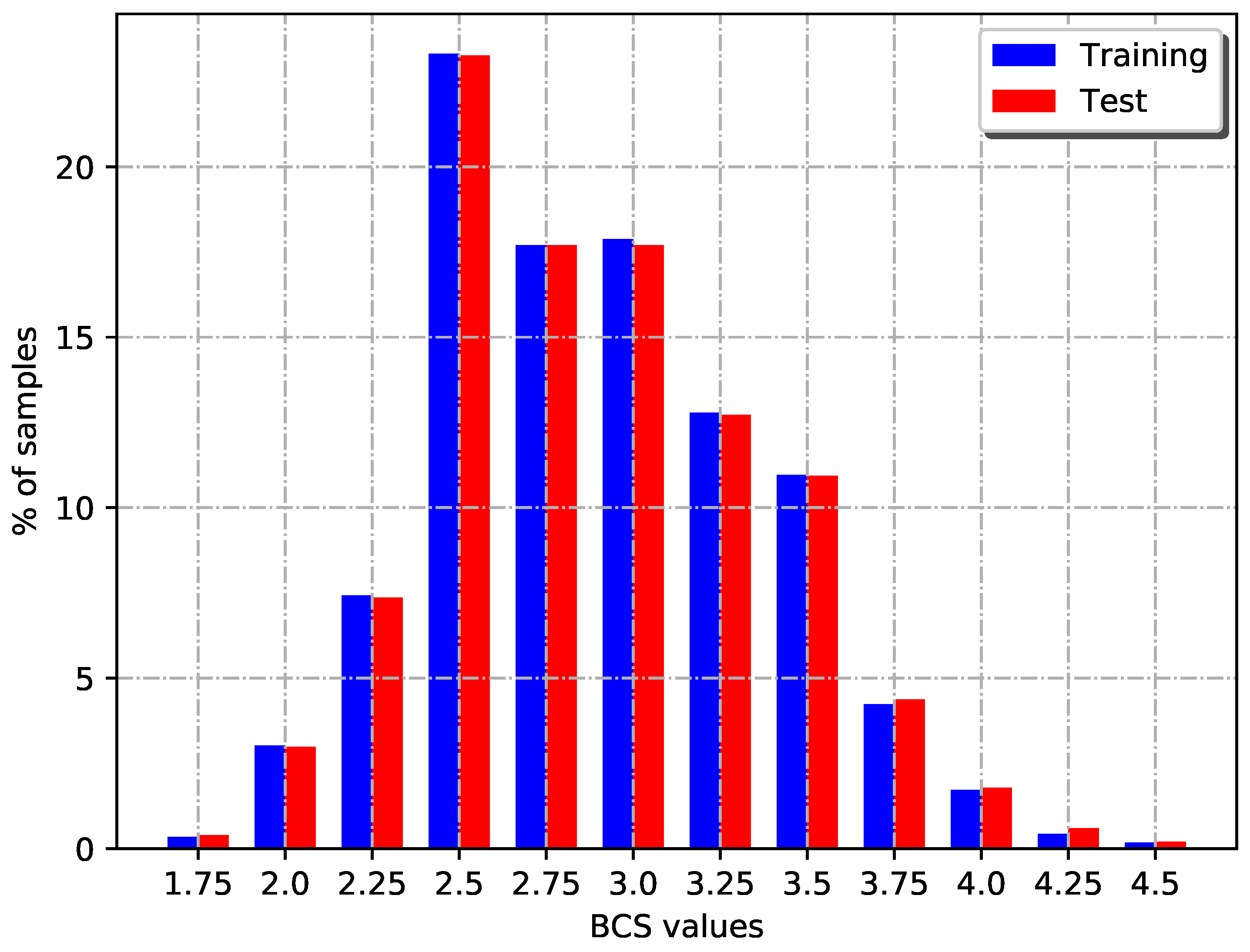
In each table, the last two rows combine per-class results to respectively calculate weighted and unweighted average metrics, i.e., these two rows present the macro-averaged classification measures of the model, considering (or not) the distribution of BCS values in the test set. Weighted metrics were added because, as it was shown before, the image dataset is imbalanced in terms of class instances.
The tables show zero values for a metric when there are not true positive values for a class. Particularly, it is possible to see that BCS = 4.5 class could not be predicted by any model irrespectively of error range. This happened because the whole dataset of images had very few samples of this class (3 in total), because of which only two samples were used to train the model to identify particular patterns, and only one sample to test them.
In general, considering confusion matrices and classification measures results, models have shown problems or difficulties to classify images on extreme BCS values, mainly in higher classes. These problems were related to low data distribution of low (emaciated) and high (fat) BCS values, because in an average livestock establishment is rare to find cows with poor body condition. This hinders the ability of models to learn features associated with extreme values, considering only a few training examples. In this sense, classes with more images to train, in the middle of the scale, present better results.
From the tables, it is possible to appreciate that two of the individual models have obtained the best results. Those were the models that transformed the depth images to generate additional channels which added extra information to assist network training. Particularly, it is important to note the incidence of the channel that highlight cow body contour, whose impact or influence on the value of the BCS has been assumed and demonstrated in different related works.
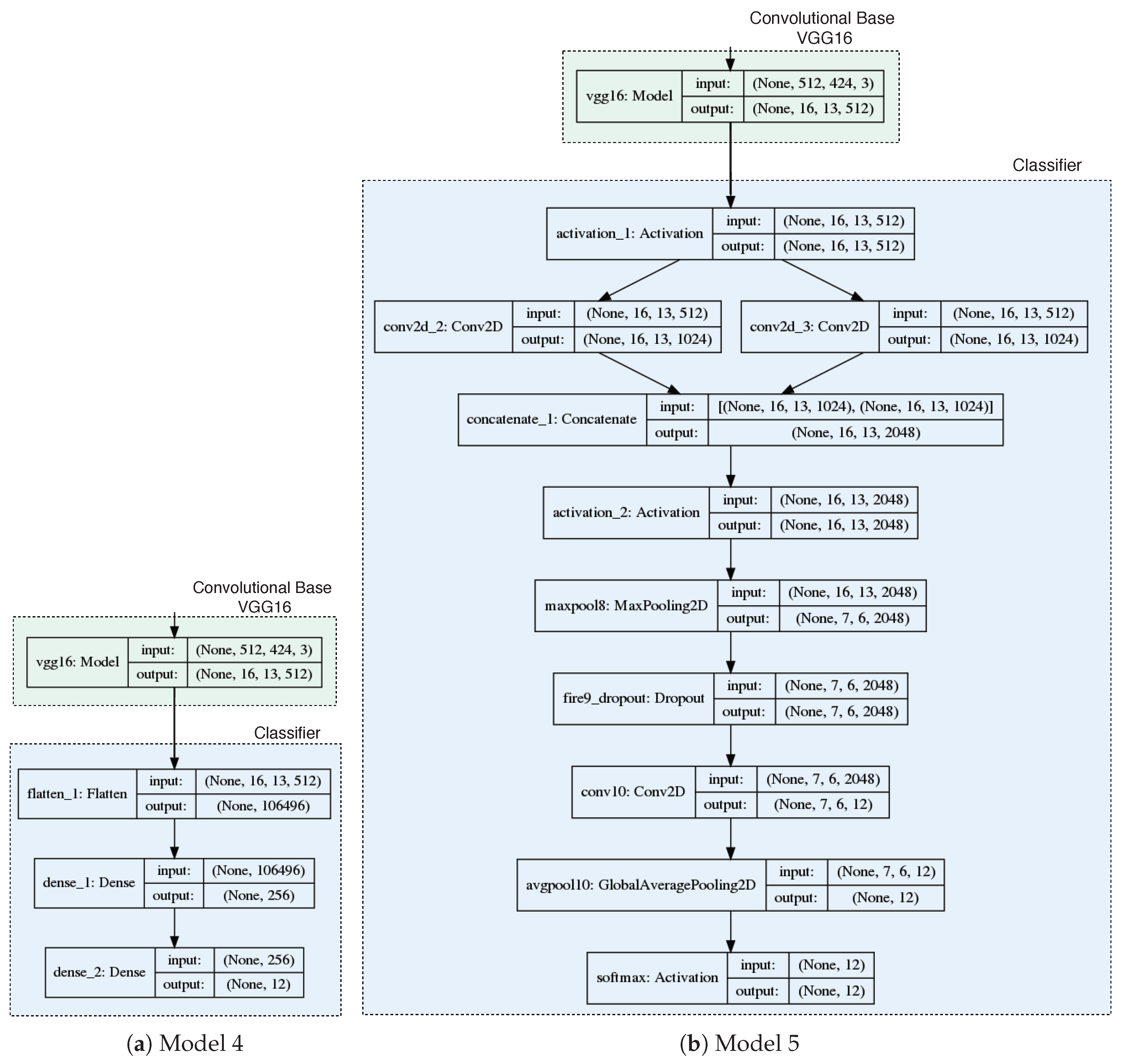
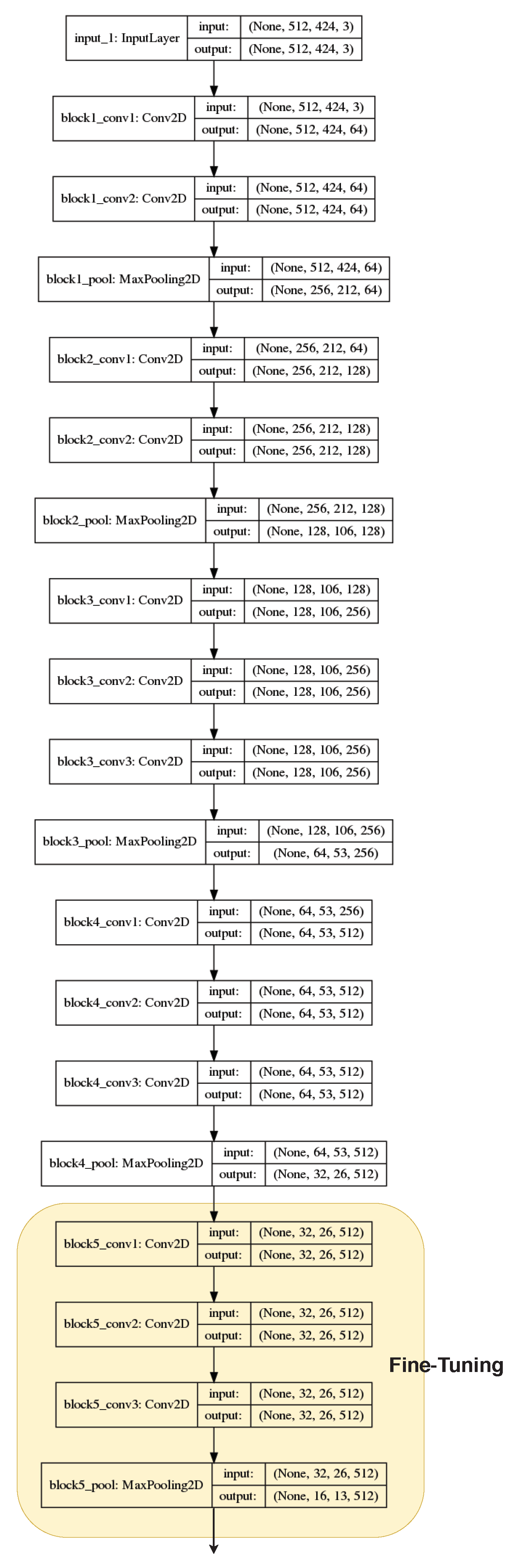
With respect to models which applied transfer learning, it was not possible to obtain the desired results and take advantage of the use of pre-trained networks over large volumes of data. At this point, the negative effect of diverse data sources was observed, corresponding to the differences between the characteristics of the images on which the weights of the VGG16 network (base) were trained and the images used in this work. The VGG16 network adjusts its weights using RGB images (with the well-known red, green and blue channels), while the cow images used in this work were composed of 3 completely different channels (Depth, Edges and Fourier). It is important to remember that we used these type of channels (i.e., channels built from depth values) instead of RGB channels because they have proven to be more suitable to depict cow body variability associated with changes in BCS [5,15]. Therefore, it was this disparity in the data sources that generates a negative impact on the final predictions.
Despite this, it was decided to test the generality and reusability of the first layers of a pre-trained deep network, fine-tuning the weights of the final layers of the VGG16 network convolutional base. Although the results improved marginally, these values did not reach those achieved by two of the models trained from scratch (Model 2 and Model 3), since the growth in the number of parameters to train produced overfitting over training set images, without contributing significantly to the generality of the model.
Although the accuracy obtained by models which applied transfer learning techniques was not as good as expected, it was decided to exploit the diversity generated and analyze if these models could contribute to give diversity to a set of predictions or model ensemble, which could allow improving the overall results of the system obtained by the best of the individual models. Thus, according to previous results and the considerations in Section 2.3.3, we define the models which compose the model ensemble as:
  • Model 2 (SqueezeNet 2 channels),
  • Model 3 (SqueezeNet 3 channels),
  • Model 6 (Fine tuning over VGG16 with a fully connected classifier),
  • Model 7 (Fine tuning over VGG16 with a classifier based on Fire modules).
Additionally, it was necessary to determine how the predictions of the models are combined to generate a new one associated with the model ensemble. The weighted average of the predictions of the individual models was chosen to calculate this value, taking into account the efficiency of each one. Table 6 shows the accuracy of each model of the ensemble and the weights assigned to each one, highlighting the importance that the best models have greater weight in the final prediction. Also, model ensemble accuracy value is shown and compared to the values achieved by its individual models. Although the improvement was small (in comparison with Model 2), these results demonstrated the importance of having an architecturally heterogeneous set of models in the model ensemble. That is, obtained results were improved even though individual models that were not as good enough as others were taken into account (particularly Model 6 and Model 7), but that allowed to add diversity to the model ensemble and counteract prediction biases. It remains to be analyzed as part of future works if these results could be even improved if models of comparable accuracy (i.e., accuracy values close to Model 2) were taken into account in the ensemble.
Similar to the analysis made in the previous work [15], overall accuracy of the best single model and the model ensemble were contrasted against works presenting medium to high BCS automatization level in the bibliography. Each related work builds and uses its own dataset to calculate this metric, i.e., there is no universal dataset of cow images that allows for a standardization of experimental factors. That is why just a high-level accuracy comparison could be made (such as those found in previous works [7,8,9,10,15]. Table 7 shows the accuracy comparison within different human error ranges, which is one of the most frequently used measure in the literature to evaluate the precision of models [3,4,7,10,24,35,36]. It is possible to appreciate how Model 2 has achieved very good results, outperforming in all cases accuracy estimations within 0.25 and 0.50 units of difference between true and predicted BCS value. However, it is important to highlight how the model ensemble has improved these results by combining different models, demonstrating a higher prediction capacity than the individual models.
An automatic estimation of BCS, as we mentioned before, already means a qualitative improvement of great impact in terms of effort, time, money and objectivity in capturing this productive variable. However, in addition, improvements in the accuracy of any of these automatic processes (such as the 3–4% achieved by this work in comparison with the previous one), which a priori seem scarce numerically, represent a great advance (especially if we take into account that quality jumps in accuracy values are reduced as they approach 100% accuracy) that allow a more precise monitoring of this indicator, which could directly impact and achieve a greater nutritional efficiency, and at the same time would lead to improve the profitability of the livestock business.
Regarding Model 8, it is true that implementing an ensemble could increase the computational cost of the solution, but as we mentioned before at this scale of accuracy each improvement represents a challenge and it is justified if the cost is not too high. In this sense, on one hand each model used by the ensemble was trained offline, and each one represented a potential solution during the learning cycle (Idea-Code new model-Training-Testing/Evaluation). Thus, at this point, the extra computational cost was just associated in order to decide how the results of the individual models should be combined to generate a more accurate final prediction. On the other hand, in practice the estimation produced by each trained model could be done in parallel, and then simply combine the values in the previously defined way.

4. Conclusions

This work has analyzed how different model configuration and machine learning techniques could be used in order to estimate BCS on cows from depth images. As base system, we employed a single-model BCS estimator that uses CNNs already proposed in [15].
Particularly, a variation on the number of input channel model has proven to get better results than the legacy model. It was possible to appreciate that the information added by Fourier channel was not relevant to this problem, since it was not reflected in an increase in model performance and could even generate an increase in preprocessing times.
The models that used the different transfer learning alternatives were not able to improve classification measures. This is due to the disparate nature of the data used to pre-train models (used to transfer knowledge) and data used to solve the current problem. At this point it may be convenient to use only part of the convolutional base of the pre-trained network, in particular some of the first layers, since they extract more generic features and they are less linked to the source problem. This would reduce the bias of the layers near the output of the convolutional base towards classes of the source task. Nevertheless, these models were useful to give diversity to an ensemble of models, improving the obtained results by any of the individual models, and validating the application of this technique. However, in future works it will be necessary to analyze if it is possible to improve the ensemble accuracy considering new models that are better than those obtained through transfer learning techniques, and achieve accuracy values comparable to Model 2. According to the shown results, these new models should be trained from scratch (as far as we know there are not CNN models trained over similar problem which could be used to transfer learning) and they should developed using different architectures or configurations (with respect to Model 2), in order to preserve models diversity in the ensemble, which has demostrated to be useful.
Summarizing, two of the model analyzed in this work have improved the results achieved by the previous work. These two models were:
  • Model 2: a model based on SqueezeNet with two input channels (Depth and Edge) trained from scratch;
  • Model 8: an ensemble which combined the two best models (Model 2 and Model 3) with two other architecturally different models (Model 6, Model 7).
However, although the results of Rodríguez Alvarez et al. [15] have been improved, at this point the need to increase the dataset is stressed, especially extreme BCS values. That is, it is necessary to have an extended data set with an equitable data distribution in order to achieve a quality jump in the system accuracy.

Author Contributions

J.R.A., M.A., J.M.R., C.M. (Claudio Machado), C.M. (Cristian Mateos) conceived the experiments and established guidance for the writing of the manuscript. J.R.A., J.T., D.J., C.S., C.M. (Claudio Machado) performed the experiments. J.R.A., P.M., J.T., D.J., A.T., C.S., C.M. (Claudio Machado) performed data collection. J.R.A. completed the system development and experimental verification. J.R.A., M.A., J.M.R., C.M. (Cristian Mateos) wrote the paper. J.R.A., M.A., J.M.R., C.M. (Cristian Mateos), C.M. (Claudio Machado), A.Z. reviewed the manuscript. M.A., A.Z., C.M. (Claudio Machado), C.M. (Cristian Mateos) supervised the work. C.M. (Claudio Machado), A.Z. acquired the necessary funding.

Funding

We acknowledge the financial support by ANPCyT through grant D-TEC 2013 Number 0005/13.

Acknowledgments

We acknowledge the donated Titan XP GPU by NVIDIA through its NVIDIA GPU Grant program.

Conflicts of Interest

The authors declare no conflict of interest.

References

  1. Wildman, E.; Jones, G.; Wagner, P.; Boman, R.; Troutt, H.; Lesch, T. A dairy cow body condition scoring system and its relationship to selected production characteristics. J. Dairy Sci. 1982, 65, 495–501. [Google Scholar] [CrossRef]
  2. Ferguson, J.; Azzaro, G.; Licitra, G. Body condition assessment using digital images. J. Dairy Sci. 2006, 89, 3833–3841. [Google Scholar] [CrossRef]
  3. Ferguson, J.D.; Galligan, D.T.; Thomsen, N. Principal descriptors of body condition score in Holstein cows. J. Dairy Sci. 1994, 77, 2695–2703. [Google Scholar] [CrossRef]
  4. Shelley, A.N. Incorporating Machine Vision in Precision Dairy Farming Technologies. Ph.D. Thesis, University of Kentucky, Lexington, KY, USA, 2016. [Google Scholar]
  5. Fischer, A.; Luginbühl, T.; Delattre, L.; Delouard, J.; Faverdin, P. Rear shape in 3 dimensions summarized by principal component analysis is a good predictor of body condition score in Holstein dairy cows. J. Dairy Sci. 2015, 98, 4465–4476. [Google Scholar] [CrossRef] [PubMed]
  6. Hansen, M.; Smith, M.; Smith, L.; Hales, I.; Forbes, D. Non-intrusive automated measurement of dairy cow body condition using 3D video. In Proceedings of the British Machine Vision Conference—Workshop of Machine Vision and Animal Behaviour, Swansea, Wales, UK, 10 September 2015; BMVA Press: Durham, England, UK, 2015; pp. 1.1–1.8. [Google Scholar]
  7. Bercovich, A.; Edan, Y.; Alchanatis, V.; Moallem, U.; Parmet, Y.; Honig, H.; Maltz, E.; Antler, A.; Halachmi, I. Development of an automatic cow body condition scoring using body shape signature and Fourier descriptors. J. Dairy Sci. 2013, 96, 8047–8059. [Google Scholar] [CrossRef] [PubMed]
  8. Halachmi, I.; Klopčič, M.; Polak, P.; Roberts, D.; Bewley, J. Automatic assessment of dairy cattle body condition score using thermal imaging. Comput. Electron. Agric. 2013, 99, 35–40. [Google Scholar] [CrossRef]
  9. Azzaro, G.; Caccamo, M.; Ferguson, J.; Battiato, S.; Farinella, G.; Guarnera, G.; Puglisi, G.; Petriglieri, R.; Licitra, G. Objective estimation of body condition score by modeling cow body shape from digital images. J. Dairy Sci. 2011, 94, 2126–2137. [Google Scholar] [CrossRef]
  10. Spoliansky, R.; Edan, Y.; Parmet, Y.; Halachmi, I. Development of automatic body condition scoring using a low-cost 3-dimensional Kinect camera. J. Dairy Sci. 2016, 99, 7714–7725. [Google Scholar] [CrossRef]
  11. Deng, L.; Yu, D. Deep learning: Methods and applications. Found. Trends® Signal Process 2014, 7, 197–387. [Google Scholar] [CrossRef]
  12. Hijazi, S.; Kumar, R.; Rowen, C. Using Convolutional Neural Networks for Image Recognition, 2015. Available online: http://site.eet-china.com/webinar/pdf/Cadence_0425_webinar_WP.pdf (accessed on 15 December 2018).
  13. Krizhevsky, A.; Sutskever, I.; Hinton, G.E. Imagenet classification with deep convolutional neural networks. Adv. Neural Inf. Process. Syst. 2012, 25, 1097–1105. [Google Scholar] [CrossRef]
  14. Szegedy, C.; Liu, W.; Jia, Y.; Sermanet, P.; Reed, S.; Anguelov, D.; Erhan, D.; Vanhoucke, V.; Rabinovich, A. Going deeper with convolutions. In Proceedings of the IEEE Conference on Computer Vision and Pattern Recognition, Boston, MA, USA, 7–12 June 2015; pp. 1–9. [Google Scholar]
  15. Rodríguez Alvarez, J.; Arroqui, M.; Mangudo, P.; Toloza, J.; Jatip, D.; Rodríguez, J.M.; Teyseyre, A.; Sanz, C.; Zunino, A.; Machado, C.; et al. Body condition estimation on cows from depth images using Convolutional Neural Networks. Comput. Electron. Agric. 2018, 155, 12–22. [Google Scholar] [CrossRef]
  16. Kamilaris, A.; Prenafeta-Boldú, F.X. Deep learning in agriculture: A survey. Comput. Electron. Agric. 2018, 147, 70–90. [Google Scholar] [CrossRef]
  17. Demmers, T.G.M.; Cao, Y.; Gauss, S.; Lowe, J.C.; Parsons, D.J.; Wathes, C.M. Neural predictive control of broiler chicken growth. IFAC Proc. Vol. 2010, 43, 311–316. [Google Scholar] [CrossRef]
  18. Demmers, T.G.M.; Gauss, S.; Wathes, C.M.; Cao, Y.; Parsons, D.J. Simultaneous monitoring and control of pig growth and ammonia emissions. In Proceedings of the Ninth International Livestock Environment Symposium (ILES IX), International Conference of Agricultural Engineering-CIGR-AgEng 2012: Agriculture and Engineering for a Healthier Life, Valencia, Spain, 8–12 July 2012. [Google Scholar]
  19. Santoni, M.M.; Sensuse, D.I.; Arymurthy, A.M.; Fanany, M.I. Cattle race classification using gray level co-occurrence matrix convolutional neural networks. Procedia Comput. Sci. 2015, 59, 493–502. [Google Scholar] [CrossRef]
  20. Pan, S.J.; Yang, Q. A survey on transfer learning. IEEE Trans. Knowl. Data Eng. 2010, 22, 1345–1359. [Google Scholar] [CrossRef]
  21. Canny, J. A computational approach to edge detection. IEEE Trans. Pattern Anal. Mach. Intell. 1986, PAMI-8, 679–698. [Google Scholar] [CrossRef]
  22. Ding, L.; Goshtasby, A. On the Canny edge detector. Pattern Recognit. 2001, 34, 721–725. [Google Scholar] [CrossRef]
  23. Iandola, F.N.; Han, S.; Moskewicz, M.W.; Ashraf, K.; Dally, W.J.; Keutzer, K. SqueezeNet: AlexNet-level accuracy with 50x fewer parameters and <0.5 MB model size. arXiv, 2016; arXiv:1602.07360. [Google Scholar]
  24. Bewley, J.; Peacock, A.; Lewis, O.; Boyce, R.; Roberts, D.; Coffey, M.; Kenyon, S.; Schutz, M. Potential for estimation of body condition scores in dairy cattle from digital images. J. Dairy Sci. 2008, 91, 3439–3453. [Google Scholar] [CrossRef]
  25. Salau, J.; Haas, J.; Junge, W.; Bauer, U.; Harms, J.; Bieletzki, S. Feasibility of automated body trait determination using the SR4K time-of-flight camera in cow barns. Springer Plus 2014, 3, 225. [Google Scholar] [CrossRef] [Green Version]
  26. Goodfellow, I.; Bengio, Y.; Courville, A. Deep Learning; MIT Press: Cambridge, MA, USA, 2016. [Google Scholar]
  27. Chollet, F. Deep Learning with Python; Manning Publications Co.: Shelter Island, NY, USA, 2017. [Google Scholar]
  28. Yosinski, J.; Clune, J.; Bengio, Y.; Lipson, H. How transferable are features in deep neural networks? Adv. Neural Inf. Process. Syst. 2014, 27, 3320–3328. [Google Scholar]
  29. Keras. 2015. Available online: https://github.com/fchollet/keras (accessed on 30 November 2018).
  30. Simonyan, K.; Zisserman, A. Very deep convolutional networks for large-scale image recognition. arXiv, 2014; arXiv:1409.1556. [Google Scholar]
  31. Stehman, S.V. Selecting and interpreting measures of thematic classification accuracy. Remote Sens. Environ. 1997, 62, 77–89. [Google Scholar] [CrossRef]
  32. Han, J.; Pei, J.; Kamber, M. Data Mining: Concepts and Techniques; Elsevier: Amsterdam, The Netherlands, 2011. [Google Scholar]
  33. Maimon, O.; Rokach, L. Data Mining and Knowledge Discovery Handbook, 2nd ed.; Springer: Berlin, Germany, 2010. [Google Scholar]
  34. Sokolova, M.; Lapalme, G. A systematic analysis of performance measures for classification tasks. Inf. Process. Manag. 2009, 45, 427–437. [Google Scholar] [CrossRef]
  35. Krukowski, M. Automatic Determination of Body Condition Score of Dairy Cows From 3D Images. Master’s Thesis, Royal Institute of Technology, School of Computer Science and Communication, Stockholm, Sweden, 2009. [Google Scholar]
  36. Anglart, D. Automatic Estimation of Body Weight and Body Condition Score in Dairy Cows Using 3D Imaging Technique. Master’s Thesis, Faculty of Veterinary Medicine and Animal Science, Swedish University of Agricultural Sciences, Uppsala, Sweden, 2010. [Google Scholar]
Figure 1. Overview of developed BCS estimation system [15].
Agronomy 09 00090 g001
Figure 2. Percentage of BCS values distribution over training and test set.
Agronomy 09 00090 g002
Figure 3. CNN architecture model implemented in previous work Rodríguez Alvarez et al. [15] (based on SqueezeNet [23]). Description of SqueezeNet “Fire” module, and structure of the CNN model from its input (preprocessed image) to the final predicted class or BCS value (class with highest probability according to the input image).
Agronomy 09 00090 g003
Figure 4. Transfer Learning: Architecture of the models taken into account. Keras support to graph models [29] was used.
Agronomy 09 00090 g004
Figure 5. Transfer learning/Fine-Tuning: Convolutional Base of VGG16 model where layers selected to re-train are highlighted in yellow. Keras support to graph models [29] was used.
Agronomy 09 00090 g005
Figure 6. Confusion matrices of test samples classification. Red cells represent exact predictions, orange cells represent predictions with 0.25 units of error, and yellow cells represent predictions with 0.50 units of error.
Agronomy 09 00090 g006
Table 1. BCS values distribution over training and test set.
BCS Value (Class)Training Values DistributionTest Values Distribution
1.7542
2.003515
2.258637
2.50270117
2.7520589
3.0020789
3.2514864
3.5012755
3.754922
4.00209
4.2553
4.5021
Table 2. Micro-averaged accuracy of individual models considering correct classifications within different human error ranges. Best results are in bold.
Accuracy (%)
Error rangeM1M2M3M4M5M6M7
0 (exact)30.0039.5635.7824.4531.4133.4030.22
0.2565.2181.3177.1360.8367.3966.6071.37
0.5089.2696.8295.8288.6789.2689.4691.85
Table 3. Classification measures for exact predictions. Best results are in bold.
BCS ValuePrecision (%)Recall (%)F1-Score (%)
M1M2M3M4M5M6M7M1M2M3M4M5M6M7M1M2M3M4M5M6M7
1.75000000000000000000000
2.0050033000100701300071201900012
2.25032332533443702714831927029191252631
2.50364743413939476451513063664446494734494945
2.75333529212632251746272825224922402824252633
3.00213930212919242042402619131020403423231614
3.25203038142227212825332725143124273519241925
3.50344342332732314245452945672937444431344330
3.7525433836604033545271814275844322422328
4.00001400000011000000120000
4.25000000000000000000000
4.50000000000000000000000
Weighted average per class273735263030333040362431333026383524282928
Unweighted average per class182325162019241523221416191714232314151817
Table 4. Classification measures within 0.25 range error. Best results are in bold.
BCS ValuePrecision (%)Recall (%)F1-Score (%)
M1M2M3M4M5M6M7M1M2M3M4M5M6M7M1M2M3M4M5M6M7
1.75001000000001000000001000000
2.0050100800010010074027001313125740002424
2.2510085948210091766876814973847081808761848773
2.50568277766562816987765981819062847766727085
2.75867882607281598289906579798384838662758069
3.00547664586958865875768055387456766967614680
3.25568783416280545981786462645358848150627154
3.50648271675346697684717175787569837169625872
3.7510081908994749159100823673774574908652827661
4.0067100881001001001002278782211221133888236203620
4.2510001000000330330000500500000
4.50000000000000000000000
Weighted average per class678178636769736581776167677165817760666570
Unweighted average per class616477485158604559663742454348606939434645
Table 5. Classification measures within 0.50 range error. Best results are in bold.
BCS ValuePrecision (%)Recall (%)F1-Score (%)
M1M2M3M4M5M6M7M1M2M3M4M5M6M7M1M2M3M4M5M6M7
1.750100100100010010001001005001001000100100670100100
2.00100100100100100100100938710040878760979310057939375
2.251009597100100100907398957884899584969688919492
2.50849897948988979098978791929687989791909097
2.751009698909396859397969689849697969793919090
3.0091999791959599999898100100989895989795979698
3.25819795738395877597959589849778979582868992
3.50819690837368859896958985918089969286797882
3.7510088911009583951001009595919195100949398938795
4.008810010010010010010078100100337889568210010050889471
4.25100100100000033673300005080500000
4.500000000000000000 0000
Weighted average per class899796898990918997968989899289979688898991
Unweighted average per class778989786977786986846466757371878567677674
Table 6. Model ensembling: accuracy of models and associated weights to individual predictions. Best results are in bold.
M2M3M6M7M8 (Ensemble)
Accuracy(%)
Error Range
0 (exact)39.5635.7833.4030.2241.15
0.2581.3177.1366.6071.3781.51
0.5096.8295.8289.4691.8597.42
Weighted predictions models0.50.30.10.1
Table 7. Overall accuracy level reported by related works and the developed system (in bold) within different human error ranges.
Error RangeKrukowski (2009)Anglart (2010)Bercovich et al. (2013)Shelley (2016)Spoliansky et al. (2016)Rodríguez Alvarez et al. (2018)Model 2 SqueezeNet (2 Channels)Model 8 Ensemble
0.2520%69%43%71.35%74%78%81%82%
0.5046%95%72%93.91%91%94%96%97%

