Multi-Temporal Agricultural Land-Cover Mapping Using Single-Year and Multi-Year Models Based on Landsat Imagery and IACS Data

Abstract

The spatial distribution and location of crops are necessary information for agricultural planning. The free availability of optical satellites such as Landsat offers an opportunity to obtain this key information. Crop type mapping using satellite data is challenged by its reliance on ground truth data. The Integrated Administration and Control System (IACS) data, submitted by farmers in Europe for subsidy payments, provide a solution to the issue of periodic field data collection. The present study tested the performance of the IACS data in the development of a generalized predictive crop type model, which is independent of the calibration year. Using the IACS polygons as objects, the mean spectral information based on four different vegetation indices and six Landsat bands were extracted for each crop type and used as predictors in a random forest model. Two modelling methods called single-year (SY) and multiple-year (MY) calibration were tested to find out their performance in the prediction of grassland, maize, summer, and winter crops. The independent validation of SY and MY resulted in a mean overall accuracy of 71.5% and 77.3%, respectively. The field-based approach of calibration used in this study dealt with the ‘salt and pepper’ effects of the pixel-based approach.

1. Introduction

The increasing world population coupled with the high demand for agricultural resources [1] require reliable data on agricultural lands for decision making and planning towards the future [2]. The knowledge on available croplands is fundamental to food security [3], sustainable cropping [4] and the maximization of food production [5]. Information about the spatial distribution of crops and the spatial extent of croplands are also essential to ascertain the impact of any human activity on croplands [6].

Reliable and accurate information about agricultural lands requires an efficient and precise approach, which remote sensing (RS) can offer [7,8,9]. RS-based methods can be used to obtain various crop information, such as crop type [10], biomass [11], or yield [12]. The advent of satellite-based optical RS has revolutionized large-scale cropland mapping and has been used in many local, regional, and global agricultural projects [4,13,14,15].

The free availability of some of these images adds to the many advantages of satellite-based optical remote sensing in agriculture [16]. Such data, which is also available for historic time periods back to the early 1970s, provides a means to study the present landscapes in relation to how they were in the past. Landsat, which is the oldest running earth monitoring program, provides a 47-year archive of satellite data of the entire earth at a 30-meter resolution. As a result, most of the crop types and other agricultural mapping studies have used Landsat images as the main data source. For instance, Lui et al., [16] used multi-temporal Landsat-8 to successfully map winter wheat in China. Maxwell et al., [17] demonstrated an effective corn classification from Landsat images through an automated process in south-central Nebraska of USA, and Yin et al., [18] used dense Landsat time series data to map agricultural and land abandonment with a high level of accuracy in the Caucasus, covering parts of Russia and Georgia. Many of these studies either employed supervised or unsupervised classification to ascertain the needed land-cover information [19,20], either at the pixel or object-based levels. Despite their accurate performances, they have some limitations [21,22]. Supervised learning always requires field information, also known as training or ground-truth data [23]. Even with the unsupervised learning, knowledge about the study area is required to assign the correct land cover type to the classification results.

A large number of studies on crop type and cropland mapping used field data from the same mapping year [24,25,26]. This way of mapping is limited in situations, where there are no ground truth data available, or data collection is impossible for the period of interest. Due to the yearly and periodic changes in cultivated crops, continuous collection of ground truth information is necessary to reliably map crop types. However, given the labor-intensive, expensive and difficult nature of ground truth data collection [27], studies such as Botkin et al., [28] and Sonobe et al., [29] have recommended research into the development of training and classification methods, which is applicable to years where field information is not available (i.e., a generalized classifier).

Given the rotation of crops on fields at different seasons and the fast changes in biomass and phenology of crops, the use of temporal information is very crucial in the discrimination of crops. Prediction of land-cover based on multi-temporal data involves the use of data from several different seasons and has proven to be effective in many studies [30,31], as it integrates the varying phenological characteristics among vegetation. Leaf pigment, water, and canopy structure are proven to relate with spectral reflectance of crops but varies at different growing seasons [32]. The use of data from a single date is known to inefficiently capture the differences among the many crops which share similar spectral characteristics [10]. Manfron et al., [33] for instance, analyzed time series of satellite images to efficiently estimate the inter-annual variability of the sowing dates of winter wheat Many other studies have employed vegetation indices such as the normalized difference vegetation index and the enhanced vegetation index to capture the seasonal dynamics of crops and other land-cover characteristics [19,34].

In Europe, there exists a remarkably rich agricultural land cover data body within the Integrated Administration and Control System (IACS), which are regularly collected by farmers as part of the subsidy payment scheme in the common agricultural policy [35]. A similar agricultural data in the United States of America is the reference data collected by the Department of Agriculture (USDA) to produce the annual crop data layer (CDL) [36]. These reference data are not available to the public, which may be the reason why the CDL has served as validation data in many crop type mapping studies [8,37]. Conversely, the IACS data can be freely obtained by scientists and research institutions for scientific purposes upon an official request. However, not much has been done with the IACS data in crop type mapping. Griffiths et al., [38] created a national single-year wall-to-wall land-cover map of Germany and used IACS data as a reference to validate some part of the study area. The study of Vuolo et al., [30] demonstrated how multi-temporal Sentinel-2 data can improve the accuracy of crop prediction when IACS data was used to independently validate the classified map. To the best of the authors’ knowledge, there is no research that has used multi-temporal IACS data as training data to develop a generalized model to predict crop types from satellite data at the field level.

Therefore, we hypothesize that the IACS data can be used to train a multi-temporal field-based model, which can predict crop types from a satellite image that is independent of the model’s training year. Hence, the calibration data, as well as the data used for testing the models, are from different years. In addressing the stated hypothesis, two different modelling approaches, i.e., multiple-year (MY) and single-year (SY) calibrations were tested in the present study. While SY models are calibrated using data from just one year, MY modelling involves model training based on data from two or more years. The SY and MY approaches have been applied in some crop mapping studies, e.g., [8], but were done at the pixel level, which is characterized by the problem of ‘salt and pepper’ effects (i.e., a misclassification of neighbouring pixels despite large similarities). On the other side, the object-based method of land cover classification, that has recently attracted considerable attention [39] as a replacement for the pixel-based [40], suffers from difficulties in the segmentation scale selection. Further, it was shown to depend on the size of the objects being mapped [41] and tend to misclassify small land-cover objects in low to medium satellite images, such as Landsat [22]. Therefore, this study employs a field/polygon-based calibration approach using the exact crop field shapes from the IACS database. Our study addresses the following questions:

(1)

How well do models based on a single year’s spectral information predict crops when tested on years not included in the model calibration process?

(2)

What is the prediction performance of models calibrated on spectral information from multiple years?

(3)

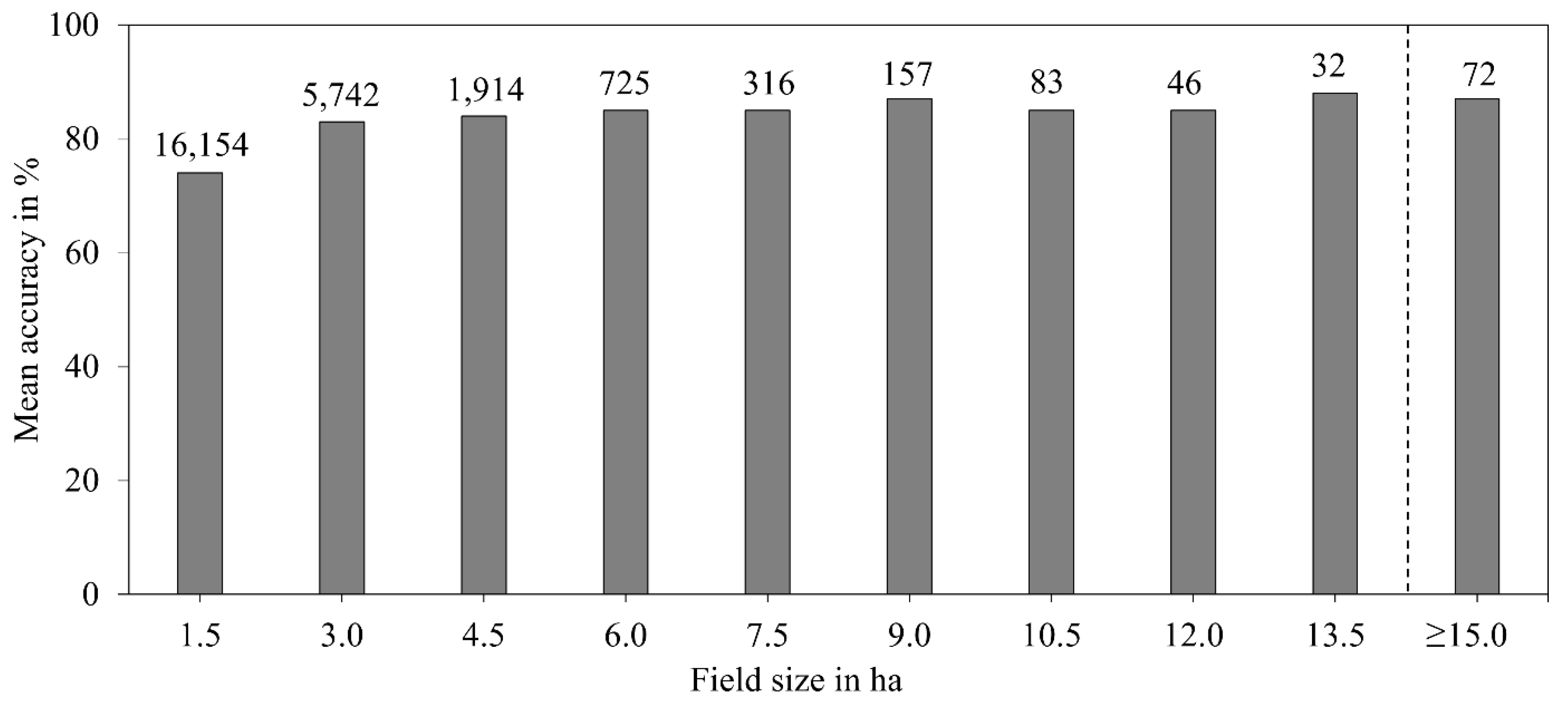
Is the accuracy of the classification models affected by field size?

2. Materials and Methods

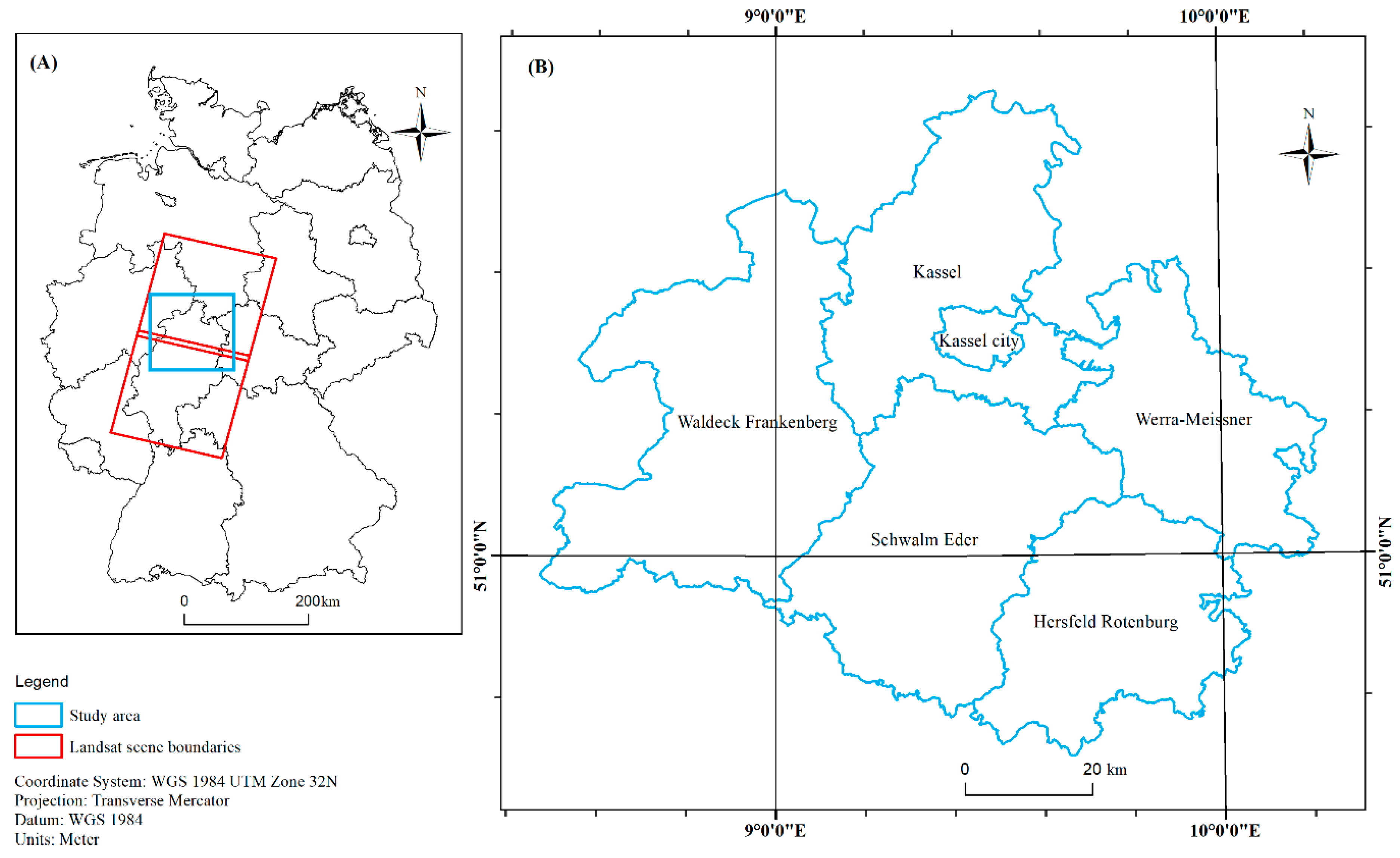
2.1. Study Area

The study was done in the Northern Hesse region of Germany (Figure 1) comprising the districts of Kassel, Waldeck-Frankenberg, Schwalm-Eder, Hersfeld Rotenburg, and Werra-Meissner. The study area comprises ca. 6900 km² and is characterized by diverse landscapes and sites with favorable and less favorable environmental conditions for farming. The favourable arable lands are mostly found in flat valleys and on plateaus with moderate slopes, which are often covered by loess of substantial thickness mainly in the western and northern parts [42]. The less favourable arable sites show shallow soils with less native water and nutrient availability.

Elevation ranges from 101 to 754 m with mean annual temperatures of 9–10 °C in the lowlands and 5–6 °C in the highlands. The mean annual rainfall ranges from 500–1300 mm [43]. The calendar of the crop types considered in this study can be seen in

Table 1. Generalized calendar of the four crop types in the study area.

Crop Types	Sowing Window	Peak Greenness	Harvesting Window
Grassland	Depending on the grassland management system
Maize	Late April	Mid-August	Mid-late September
Summer crops	Late March-Mid April	Mid-Late June	July-September
Winter crops	September-October	Mid-June	July-August

.

2.2. Data

2.2.1. Satellite Data

A total of 63 satellite images from the period April to October between 2005 and 2015 were used for this study. Surface reflectance Landsat scenes (Level-2) as summarized in

Table 2. Summary of satellite images used. (TM: Thematic Mapper, ETM+: Enhanced Thematic Mapper plus). The numbers in brackets represent the number of images used per date.

		Date of Image Acquisition
Year	Satellite	Early Summer	Late Summer
2005	Landsat 5 TM	03-Apr. (1), 21-Apr. (2)	18-Aug. (2)
	Landsat 7 ETM+	4-Apr. (2)
2007	Landsat 5 TM	02-Apr. (2), 25-Apr. (1), 27-Apr. (1)	16-Jul. (2), 01-Aug. (1), 24-Aug. (2)
	Landsat 7 ETM+	26-Apr (2)
2009	Landsat 5 TM	07-Apr. (2), 14-Apr. (2), 16-Apr. (2), 02-May (1), 25-May (1)	06-Aug. (2), 20-Aug. (2)
	Landsat 7 ETM+		05-Aug. (1), 22-Sep. (1)
2010	Landsat 5 TM	17- Apr. (2), 19-Apr. (2)	08-Jul. (1), 31-Jul. (1), 07-Aug. (2)
	Landsat 7 ETM+	18-Apr. (2)
2011	Landsat 5 TM	20-Apr. (1), 22-Apr. (2), 08-May (1)	03-Aug. (1), 15-Oct. (1), 22-Oct. (1)
	Landsat 7 ETM+	21-Apr. (2), 07-May(2)	20-Aug. (1), 03-Sep. (2), 21-Sep (1), 28-Sep. (2)
2015	Landsat 8	24-Apr. (2)	30-Aug. (2)

were downloaded from USGS’s Earth Explorer [44]. Images from only six years were used because of little to no clouds. The images of Landsat 5 TM and 7 ETM+ had been atmospherically corrected using Landsat Ecosystem Disturbances Adaptive Processing System (LEDAPS) by NASA [45]. Surface reflectance of Landsat-8 was produced using Landsat Surface Reflectance Code [46].

Table 3. Summary of the six spectral bands of the Landsat 5, 7 and 8. NIR = Near infra-red, SWIR = Shortwave infra-red, TM = Thematic Mapper, ETM+ = Enhanced Thematic Mapper plus.

Landsat 5 TM and 7 ETM+			Landsat 8
Band Number	Band Name	Wavelength (μm)	Band Number	Band Name	Wavelength (μm)
Band 1	Blue	0.441–0.514	Band 2	Blue	0.452–0.512
Band 2	Green	0.519–0.601	Band 3	Green	0.533–0.590
Band 3	Red	0.631–0.692	Band 4	Red	0.636–0.673
Band 4	NIR	0.772–0.898	Band 5	NIR	0.851–0.879
Band 5	SWIR-1	1.547–1.749	Band 6	SWIR-1	1.566–1.651
Band 7	SWIR-2	2.064–2.345	Band 7	SWIR-2	2.107–2.294

shows detailed information about the six spectral bands of the Landsat data used. Despite the small differences in the spectral ranges of the Landsat types, which have been well studied [47,48] to be smaller than 1 standard deviation of time-series of the spectral curve had no significant effect on classification results. Additionally, according to USGS [49], the Level-2 product (surface reflectance) of the Landsat images are similar, therefore, the Landsat data was not normalized. The atmospherically corrected Landsat images were accompanied by cloud mask layers. The images were categorized according to the dates when the images were captured, i.e., early summer (ES, April to May) and late summer (LS, July to October). ES and LS seasons cover the growing period of crop types in the study area; hence their use can help capture the different phenology of the crops at different stages of their development.

2.2.2. Reference Data

The IACS data were used as ancillary data in this study. These are spatial data collected by farmers as part of the subsidy support system within the EU. It is made up of the shapes of agricultural fields and the crop types planted in each cropping season. The models were initially developed to predict individual crop species in the study area, but tests (not shown) exhibited incorrect predictions among crops species of similar spectral characteristics and growing periods. Therefore, several crops were grouped into four crop types. They were grassland, maize, summer, and winter crops with their vegetation profiles shown in Figure 2. These vegetation profiles depict the spectral characteristics of the crop types at different stages of their development and show a similar trend across all years. Farmers are not obliged to register their fields; except for farmers who apply for subsidies. Therefore, the reference data used in this study is limited to the declared fields as submitted to the responsible agency. Fallow fields were not considered in this study since the reference data (i.e., the IACS) used for modelling consists of only cultivated fields.

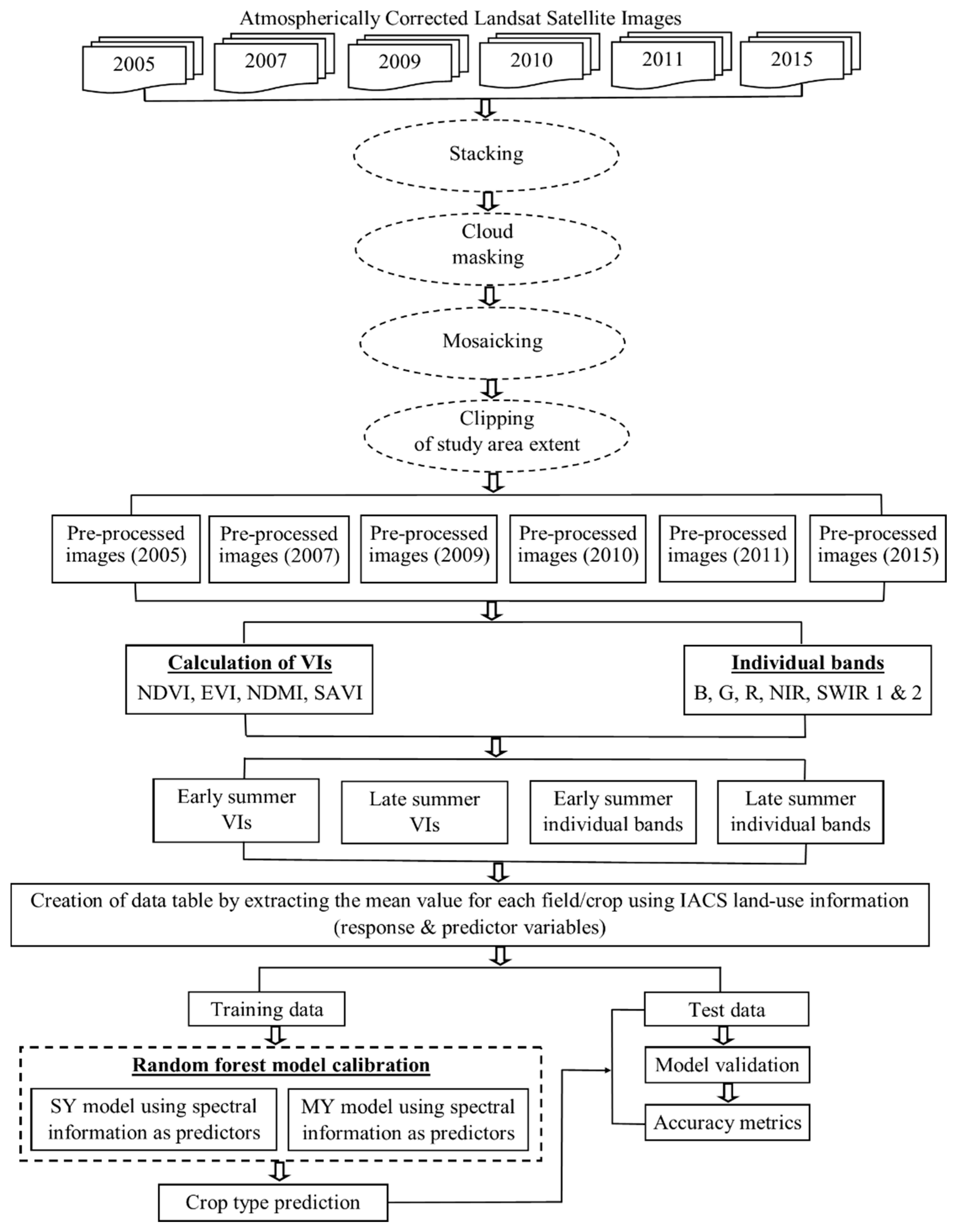
2.3. Data Processing

Image Pre-processing

The different bands (i.e., blue, green, red, near infra-red and shortwave infra-red 1 and 2) of the satellite images were stacked together, based on the years and acquisition time (Figure 3). Some of the images had small areas of clouds since cloud cover of less than 10% was considered appropriate for the study purpose. As a result, the cloud masks that came with the images were used to mask out all clouds. The masked areas were replaced with non-cloudy data from other images of the same area around the same time frame (i.e., May for ES and September, October for LS). With respect to the Landsat 7, the scan lines which resulted from the failure of the scan line corrector of the ETM+ sensor were also replaced with cloud-free satellite data from other images of the same area using the “cover” function [50] from the “raster” package in R software [51]. As our study area includes more than one Landsat image, some images were mosaicked to cover the entire area of interest. Mean values were used for overlapping layers during the mosaicking process. Figure 3 shows a complete workflow of the data analysis of this study.

2.4. Model Calibration and Validation

Crop type prediction models were built based on random forest (RF) algorithm, which is an ensemble supervised machine learning classifier that creates numerous decision trees for prediction by randomly selecting subsets of the training data through the process of bagging [52]. Higher accuracies have been achieved with RF as compared to other machine learning algorithms in many crop mapping studies [7,8]. It can effectively function with only two main parameters, i.e., the number of trees to grow (Ntree) and the number of predictor variables selected for the best splitting of each tree node (Mtry) [53]. In this study, Ntree was set at 500 for all models since the error steadies before this number is reached, while Mtry was set to the square root of the input variables as reviewed by Belgiu and Drăgu [53].

2.4.1. Input Variables Used in the Model

Spectral data obtained from the satellite data and used as predictors in the crop type predictive models consisted of blue, green, red, near infra-red (NIR), shortwave infra-red 1 (SWIR 1) and shortwave infra-red 2 (SWIR 2). Additionally, four widely used spectral vegetation indices (VIs), i.e., normalized difference vegetation index (NDVI) [54], enhanced vegetation index (EVI) [34], soil adjusted vegetation index (SAVI) [55] and normalized difference moisture index (NDMI) [56], were computed from a ratio of different satellite bands (see Equations (1)–(4)) and included as explanatory variables. These VIs capture the dynamics of vegetation like greenness and vigor among others at different phenological stages. The potential of NDVI to assess vegetation dynamics of crops has been demonstrated by a number of studies [10,19]. However, it has shortcomings of sensitivity to saturation, soil background effects, or atmospheric effects. In dealing with these limitations, EVI and SAVI were added. SAVI deals with the soil background effects, while EVI uses the blue band to deal with the atmospheric influences by aerosols. EVI, NDVI, and SAVI, as shown in Equations (1)–(3), respectively, use the NIR and red bands in their computation, and they complement each other when used in vegetation analysis. NDMI, which uses NIR and SWIR for measuring the water content in vegetation, was also included in the analysis (Equation (4)), as it adds some complementary information to the other VIs.

NDVI = (NIR − Red)/(NIR + Red)

(1)

EVI = G × (NIR − Red)/(NIR + C₁ × Red − C₂ × Blue + L)

(2)

SAVI = [(NIR − Red)/(NIR + Red + L)] × (1+ L)

(3)

NDMI = (NIR − SWIR)/(NIR + SWIR)

(4)

where NIR = Near Infra-red, G = gain factor, C₁ and C₂ are aerosol resistance term coefficients, L in Equation (2) is non-linear canopy background adjustment, L in Equation (3) is soil brightness factor and SWIR = Shortwave Infra − red (values: G = 2.5, C₁ = 6, C₂ = 7.5, L_EVI = 1, L_SAVI = 0.5).

2.4.2. Field-based Extraction of Spectral Information.

The extraction of the spectral information was done at field base with the exact crop fields as objects. Mean values of each crop’s field were extracted from the spectral data, which consisted of six individual bands of the satellite image, as well as four vegetation indices; grouped into early summer (ES) and late summer (LS) spectral information. In all, 20 different spectral information were used as predictors in the RF models. Since the IACS data (Figure 5) represent field information and, crops are cultivated with unequal distribution of fields for each crop type, almost equal numbers of polygon/field samples for each crop type were selected. Thus, crop types with many fields were always undersampled compared to those which were represented by fewer fields. Six different data tables were built for the six respective years, which were later used to calibrate and validate the crop type prediction model, with the spectral information and crop types as predictor and response variables, respectively.

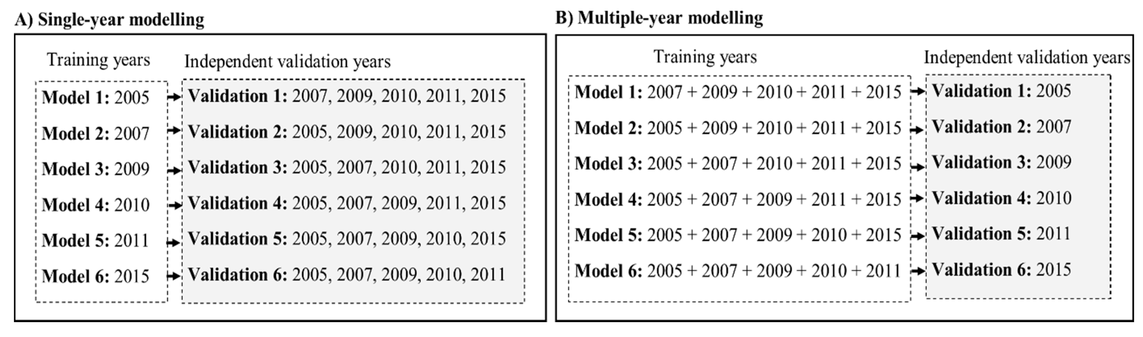
2.4.3. Crop Type Prediction Modelling

Two different modelling approaches called same-year (SY) and multiple-year (MY) training were employed. With respect to SY models, an RF algorithm was trained using only the spectral information of one year and cross-validated using the remaining years as shown in Figure 4A. This was repeated six times, where for each repetition a different year was used to train the model, and the model’s performance in predicting crop types was assessed using the remaining single-year data.

MY models were trained by combining the extracted spectral information from five different years during the training phase and tested on an independent year. The training combination with multiple years was done six times, and with each repetition a single year was left out to validate the efficacy of the MY models (Figure 4B). The contribution of the predictors was assessed based on the internal mean decrease Gini of RF, which is the average of all Gini impurity recorded for each input variable when selected for splitting at each tree node [57]. Graphs showing the six most important predictor variables (based on percentages of the mean decrease Gini Index) of the best modelling method were created for visualization.

2.4.4. Accuracy Assessment

The performance of the models in predicting crop types was independently evaluated at field scale based on a confusion matrix. The independent validation was done by comparing the predicted crop types with the known crops using the reference data. The three most important and widely used metrics namely, overall accuracy (OA), user accuracy (UA) and producer accuracy (PA), resulting from the confusion matrix were calculated. OA assesses the overall performance of a model and is the ratio of correctly predicted crops and the total number of predicted crops. UA evaluates how well the predicted crops agree with the known reference data (i.e., the IACS field data), while PA measures the agreement between the reference data and the prediction. From the confusion matrix, the error of commission (EC) and error of omission (EO) of the respective land cover types can be obtained. Since the performance of each developed SY model was tested for all years, except for the training years, the presented accuracy measures are averages of OA, UA, and PA of the same years. Since accuracies and errors of spatial data are spatially explicit, a map was created that demonstrates our models’ ability to visualize correctly and wrongly predicted fields using the best modelling method.

2.5. Relationship between Field Size and Accuracy

To check whether the accuracy of crop type prediction depended on the size of crop fields, the correctly and wrongly predicted fields along with their sizes were extracted for each of the MY models. Field sizes were rounded to the nearest multiples of 1.5 ha (i.e., the average field size) to create field size classes, with the count of the all correct (True) and wrong (False) predictions for each field size category. The percentages of correct predictions for all the field size categories were computed.

3. Results

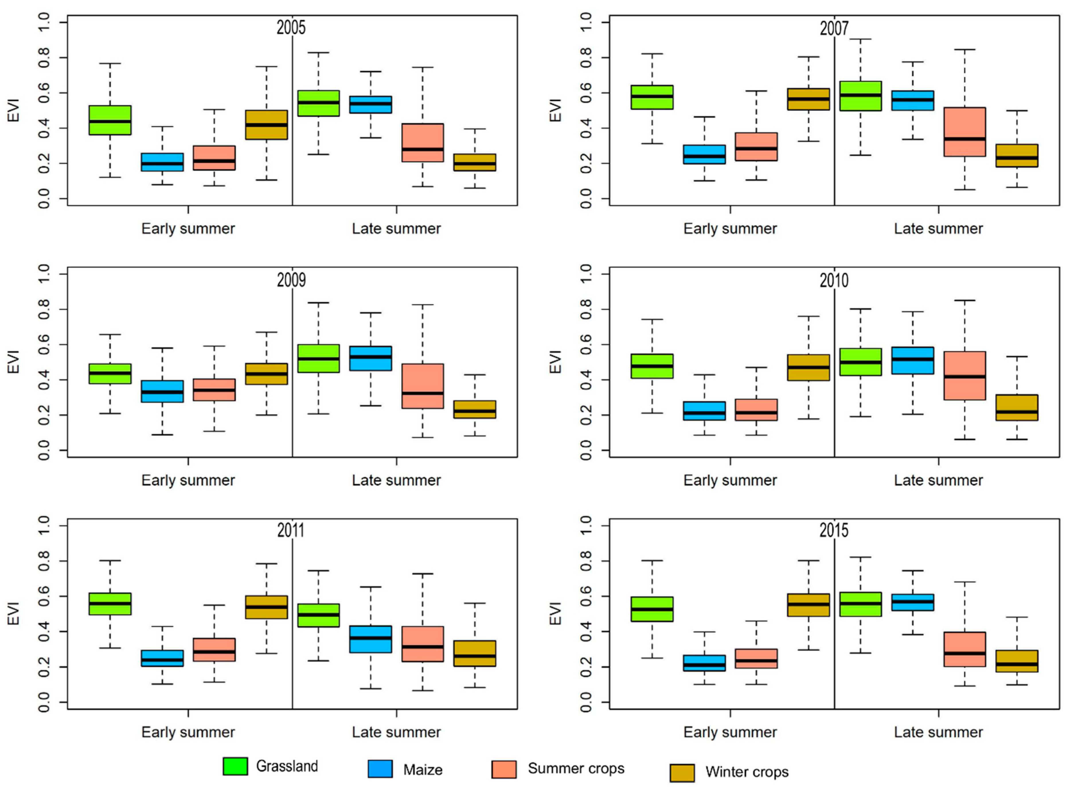
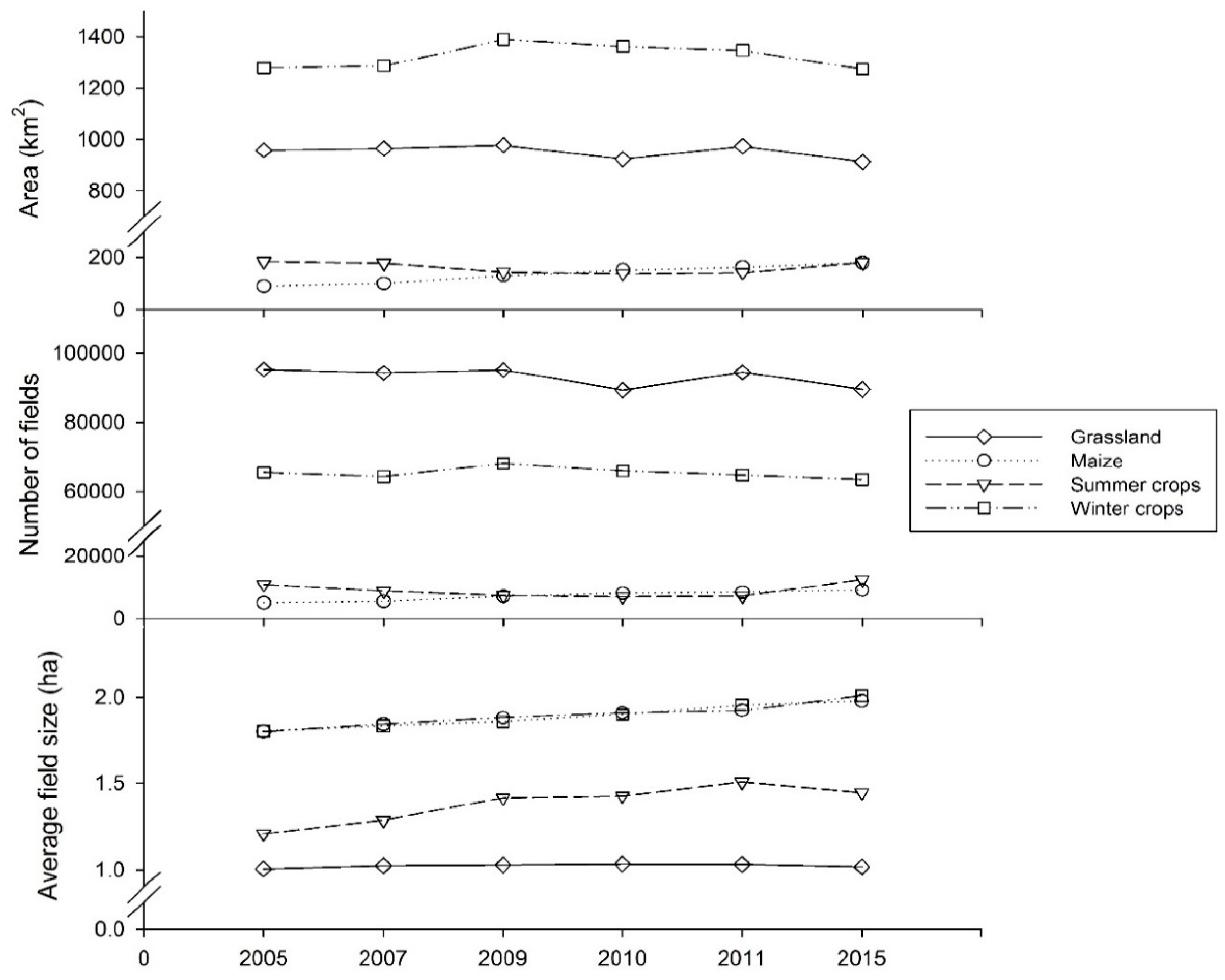
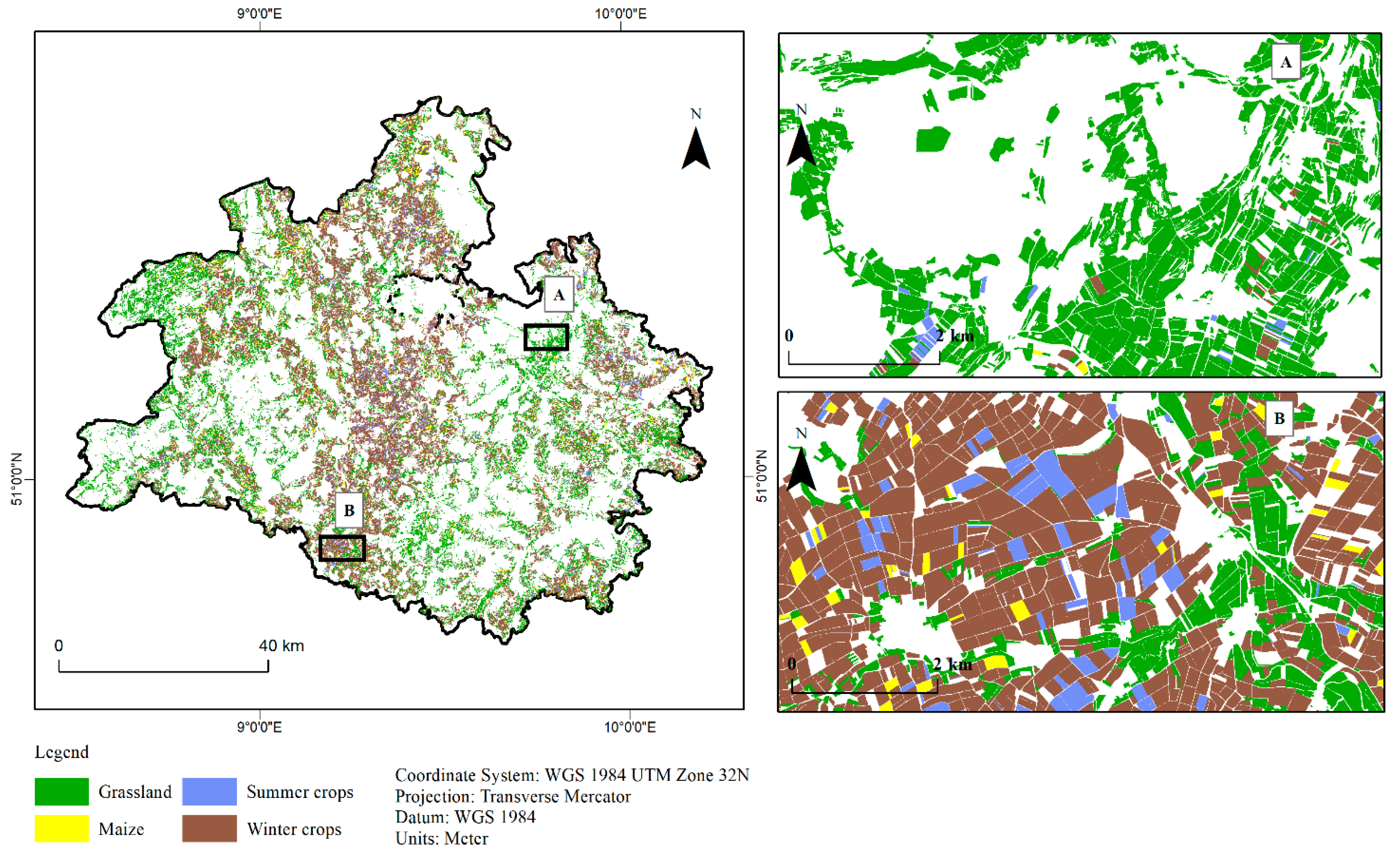
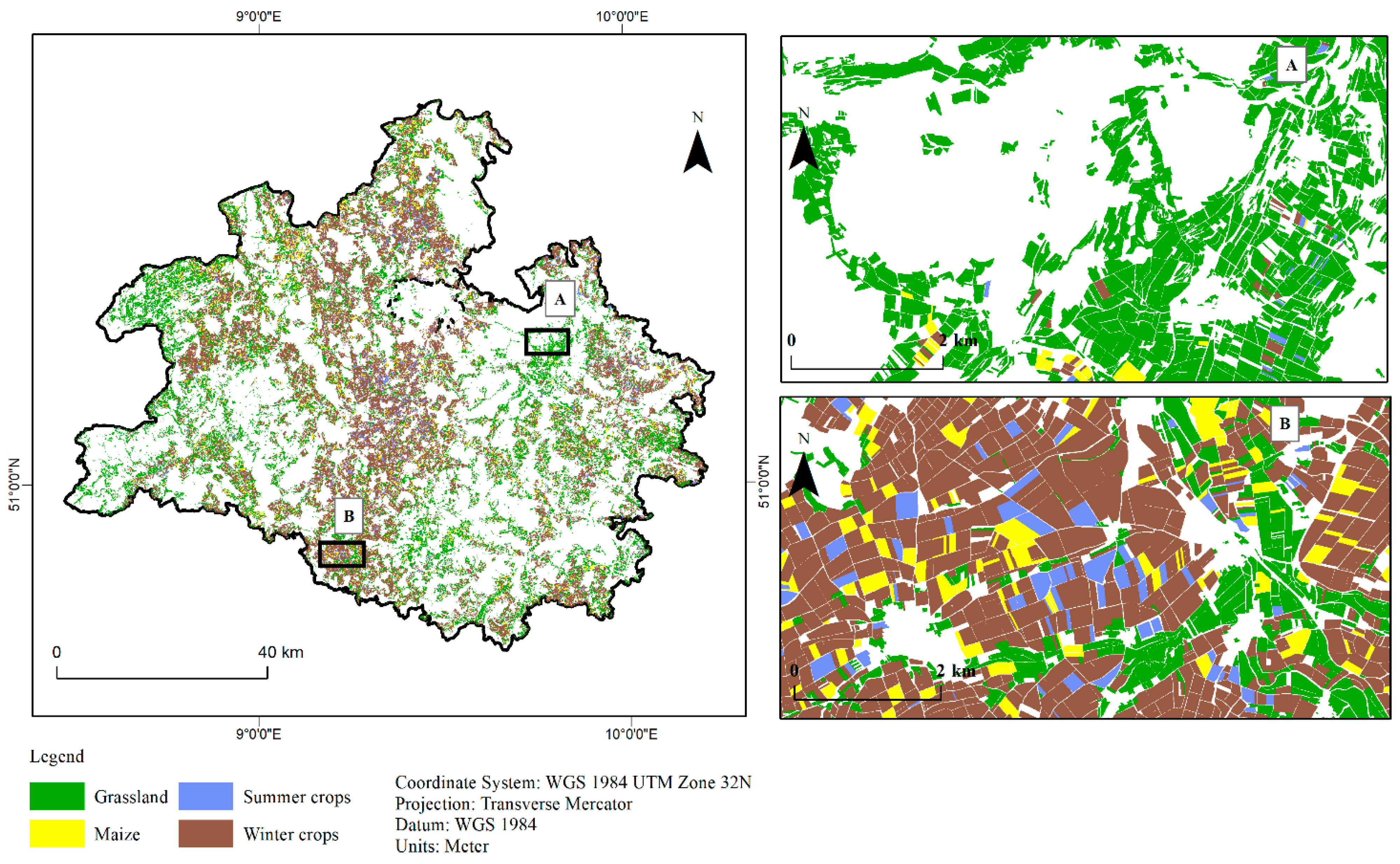
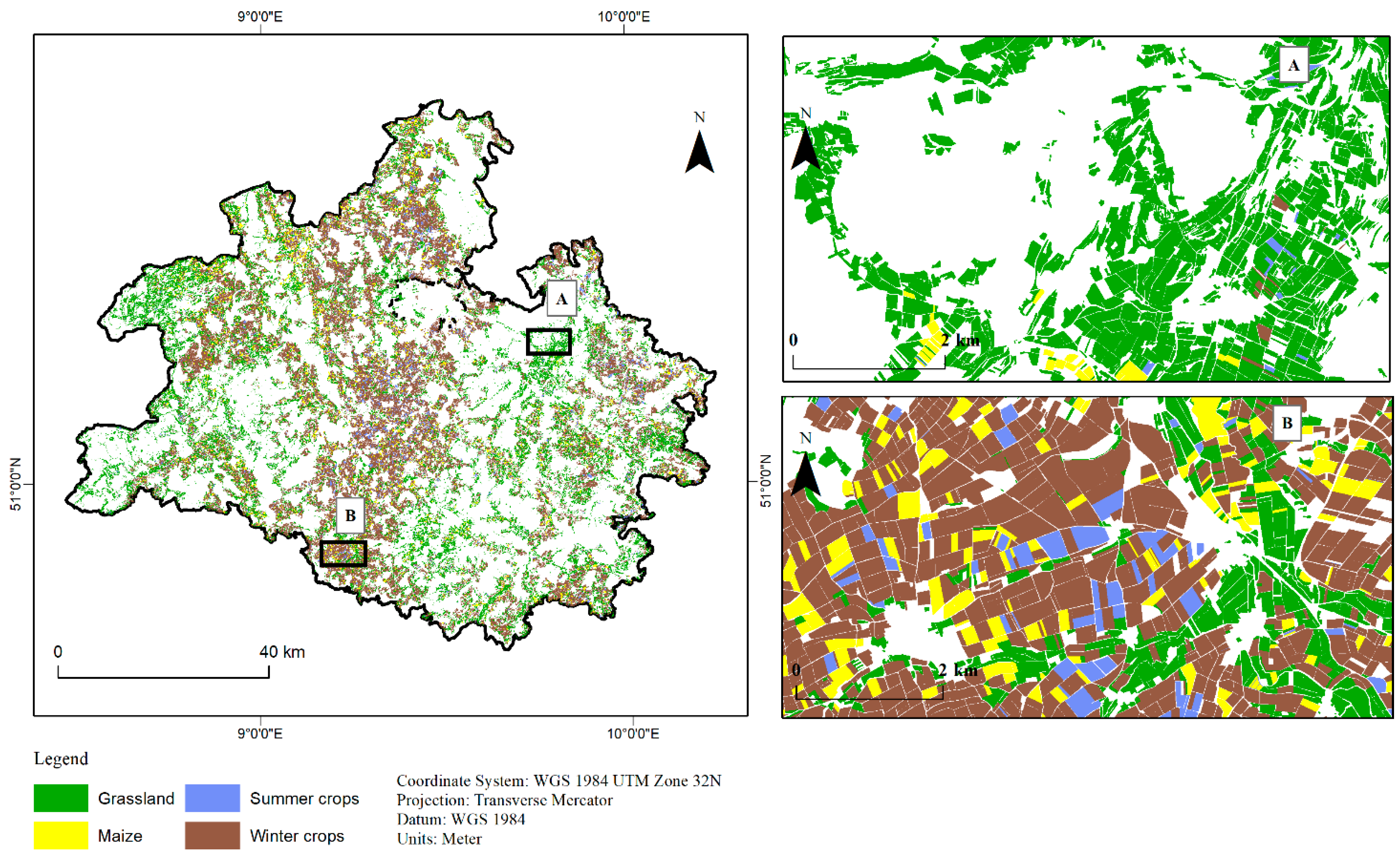
3.1. Agricultural Land Cover Data

The IACS data used as reference data to calibrate and validate the developed models showed different field numbers, average field size, and area for grassland, maize, summer crops, and winter crops (Figure 5). The average field size for grassland was around 1 ha and did not change significantly over time. Summer crops showed a slightly higher average field size between 1.2 and 1.5 ha for all years under consideration. Maize and winter crops had the biggest average field sizes, ranging between 1.8 ha to 2 ha from 2005 to 2015.

While grassland had the highest number of fields followed by winter crops, the number of maize and summer crops were the lowest. Consequently, winter crops covered the largest area of arable lands in the study area followed by grassland, whereas the area of maize and summer crops was comparatively small.

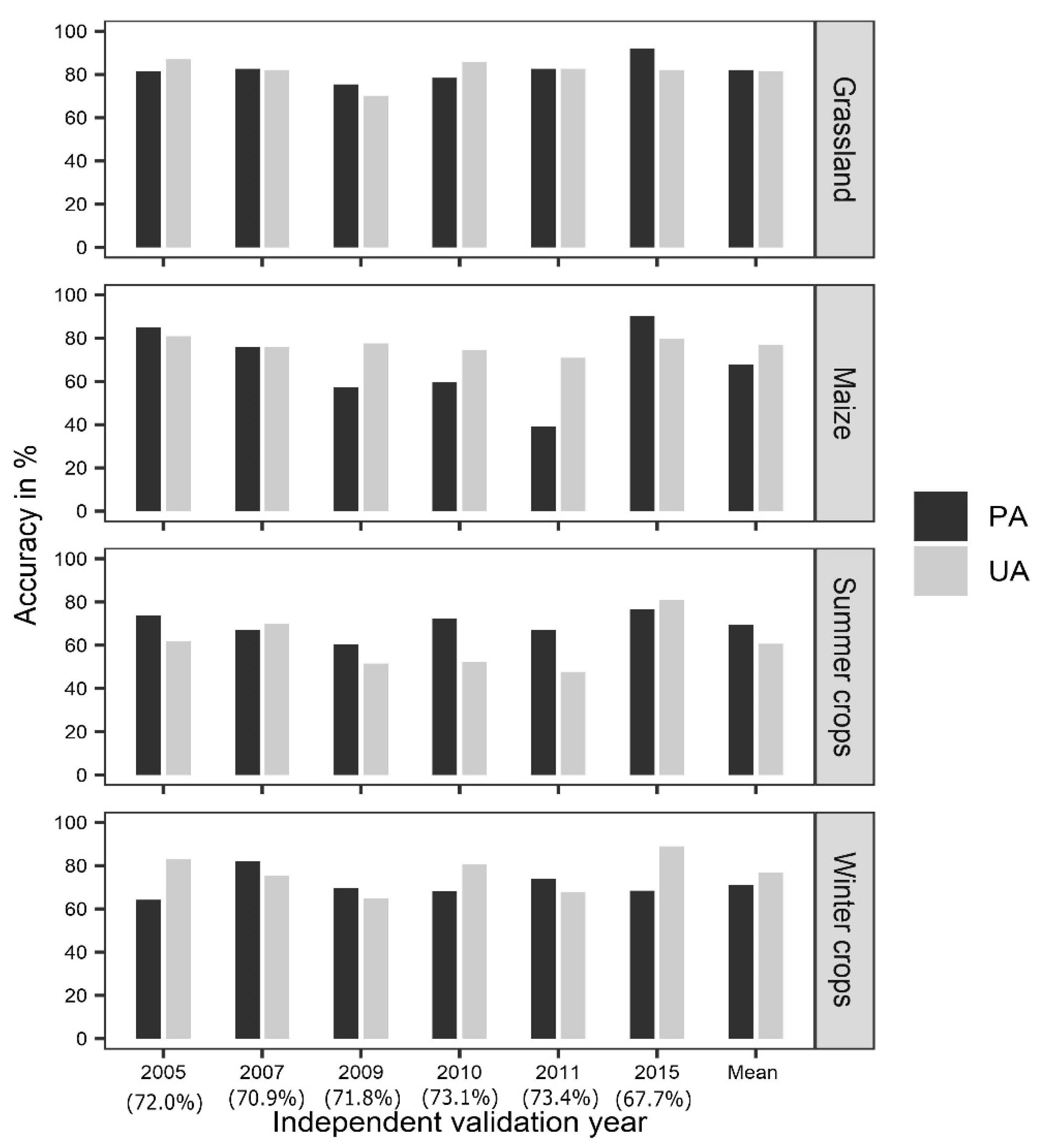
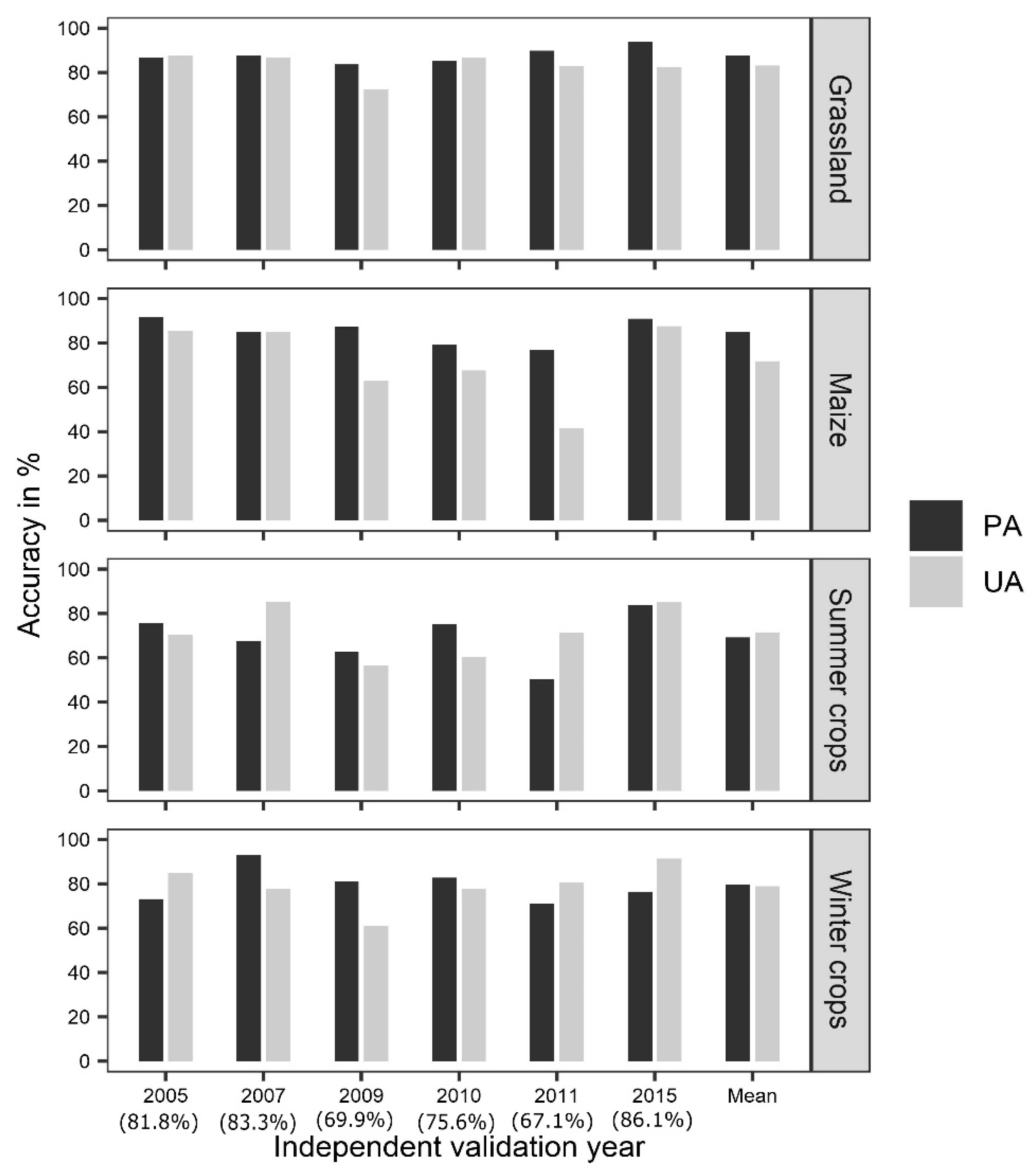
3.2. Assessment of the Modelling Approaches

The general performance of the two modelling approaches as indicated by the OA (Figure 6) ranged from 67.7% to 73.4% with an average value of 71.5% for the SY models. The MY modelling approach showed an OA between 67.1% and 86.1% with an average of 77.3% (Figure 7). The lowest OA for the SY models was observed when they were tested with crops in the year 2015, while the highest OA value was achieved in 2011. Conversely, MY models achieved their highest OA in 2015, whereas, the lowest performance was observed in 2011.

The SY prediction of individual crop types in different years based on user (UA) and producer accuracy (PA) showed a high UA (81.6%) and PA (82.2%) values for grassland, while UA (76.7%) and PA values (67%) for maize were somewhat lower. Prediction of summer crops (UA and PA of 60.6 % and 69.5 % respectively) was less accurate than winter crops (UA 76%, PA 71.1%).

The application of MY models to identify grassland area of different years resulted in a mean UA of 83.1% and a PA of 87.8% (Figure 7). Maize was discriminated with a mean UA and PA of 71.8% and 85.2% respectively, while winter crops were discriminated with a mean accuracy of 79% (UA) and 79.6% (PA). The average accuracy for summer crops was comparatively low (PA = 71.5% and PA = 69.3%), which was mainly a result of the confusion between summer crops and the other crops.

Overall, grasslands always exhibited higher accuracies (UA and PA > 80%) across years when predicted by the two modelling methods, whereas the arable crops were better predicted by the MY models in comparison to the SY models.

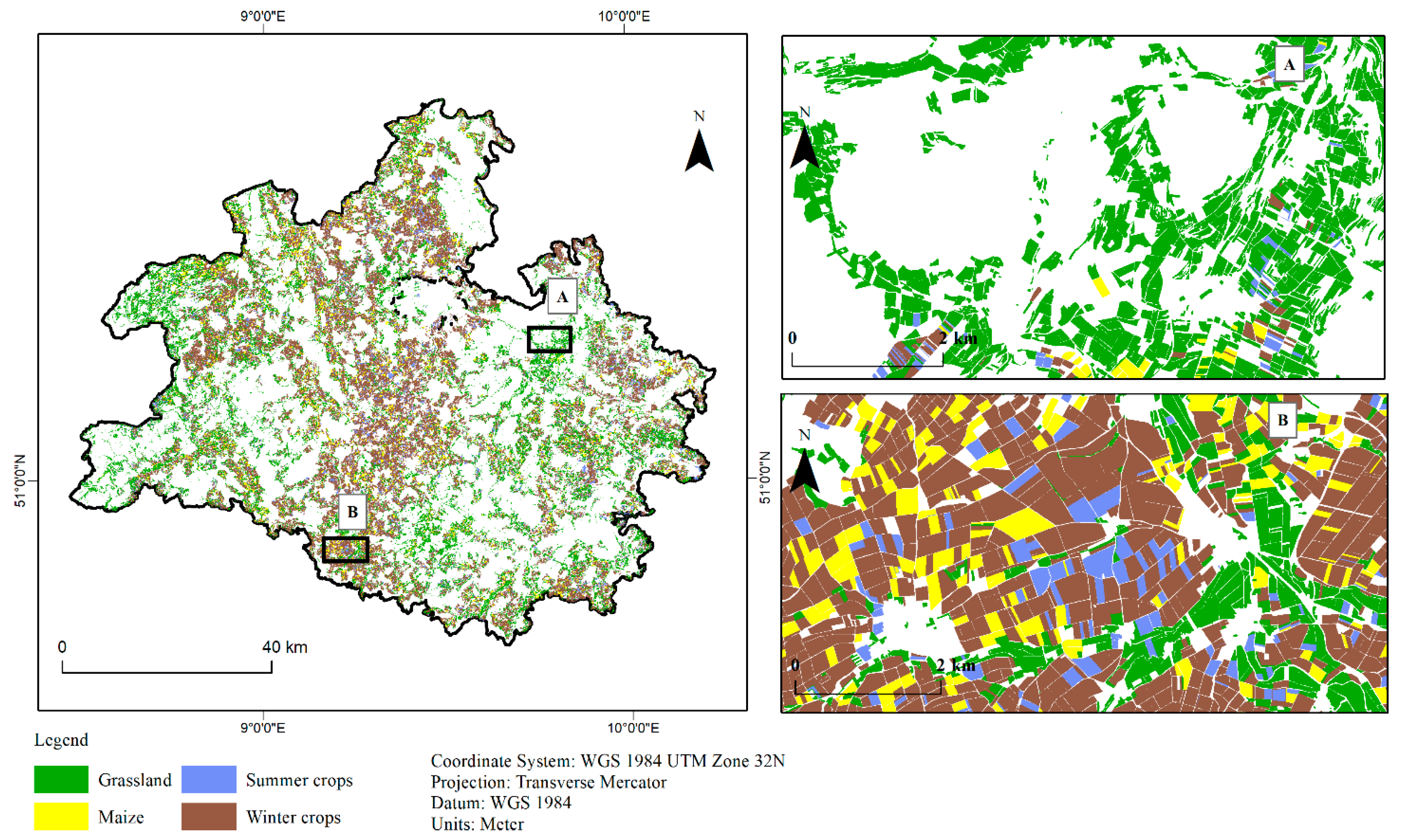
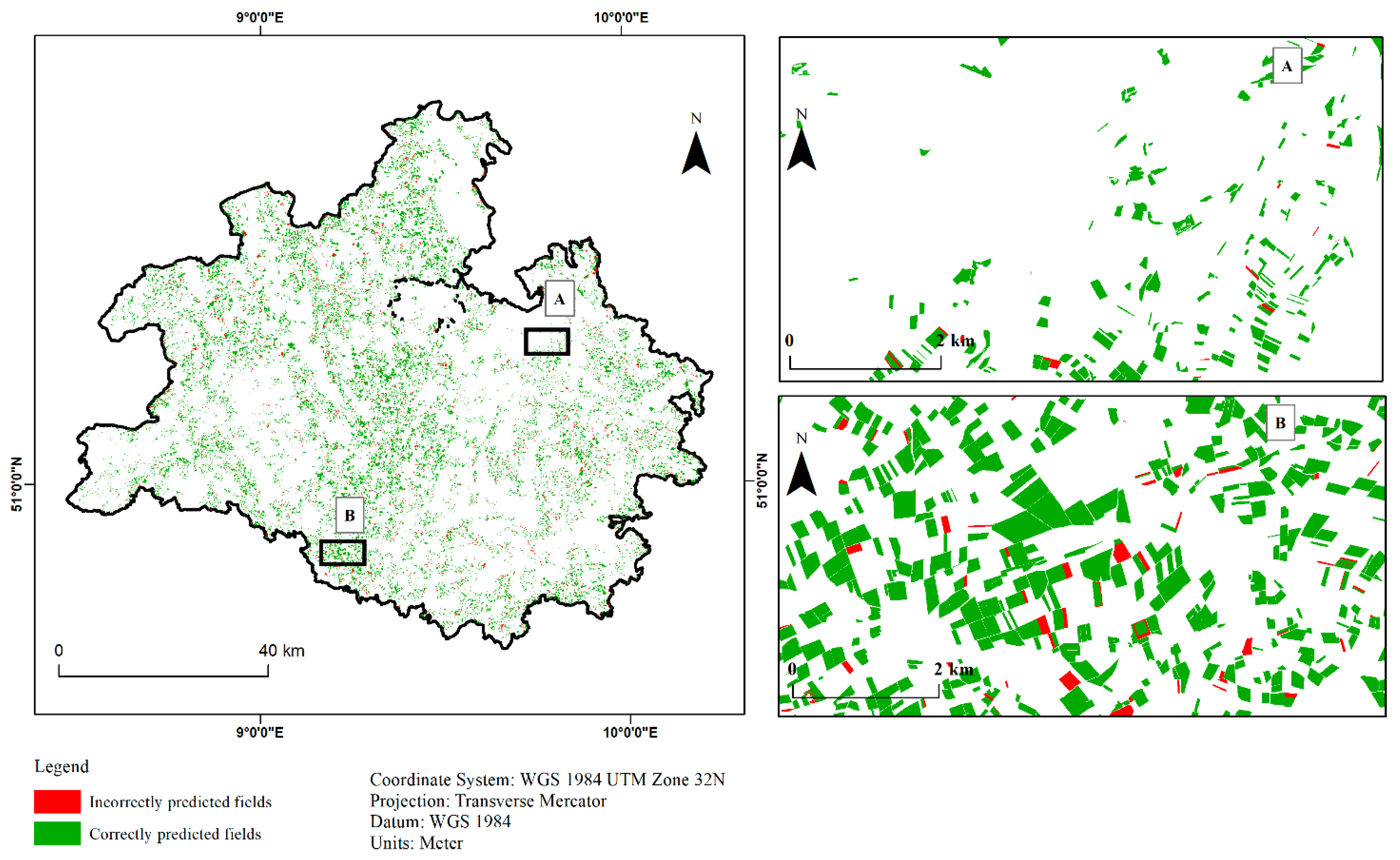
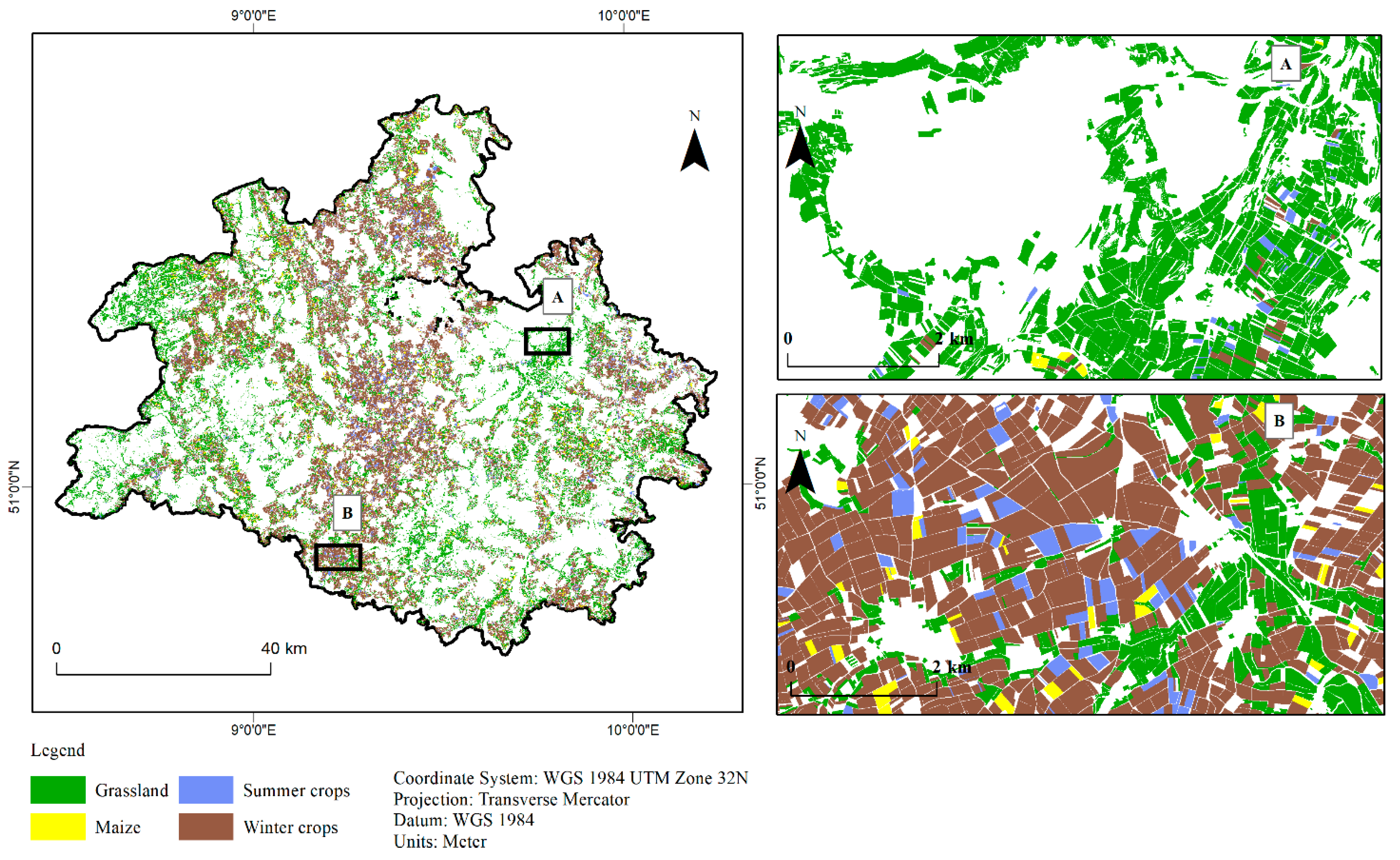
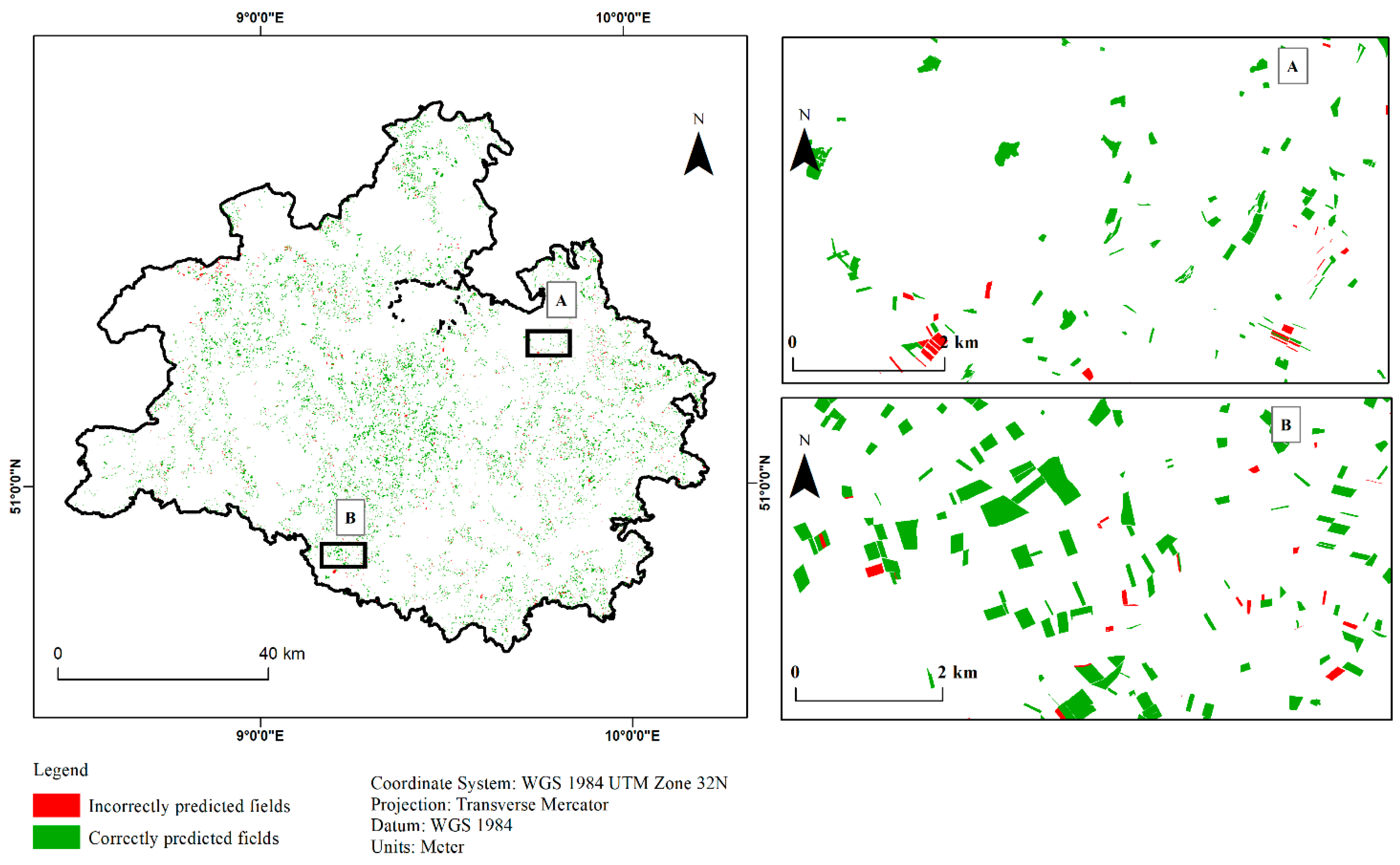
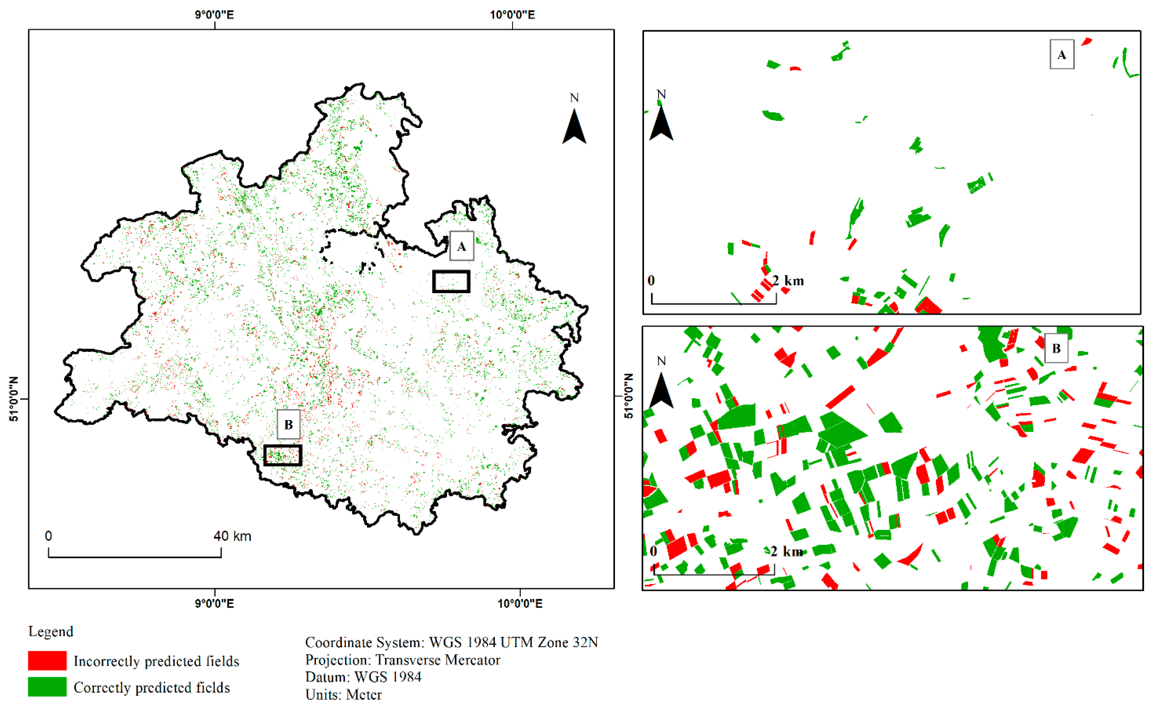
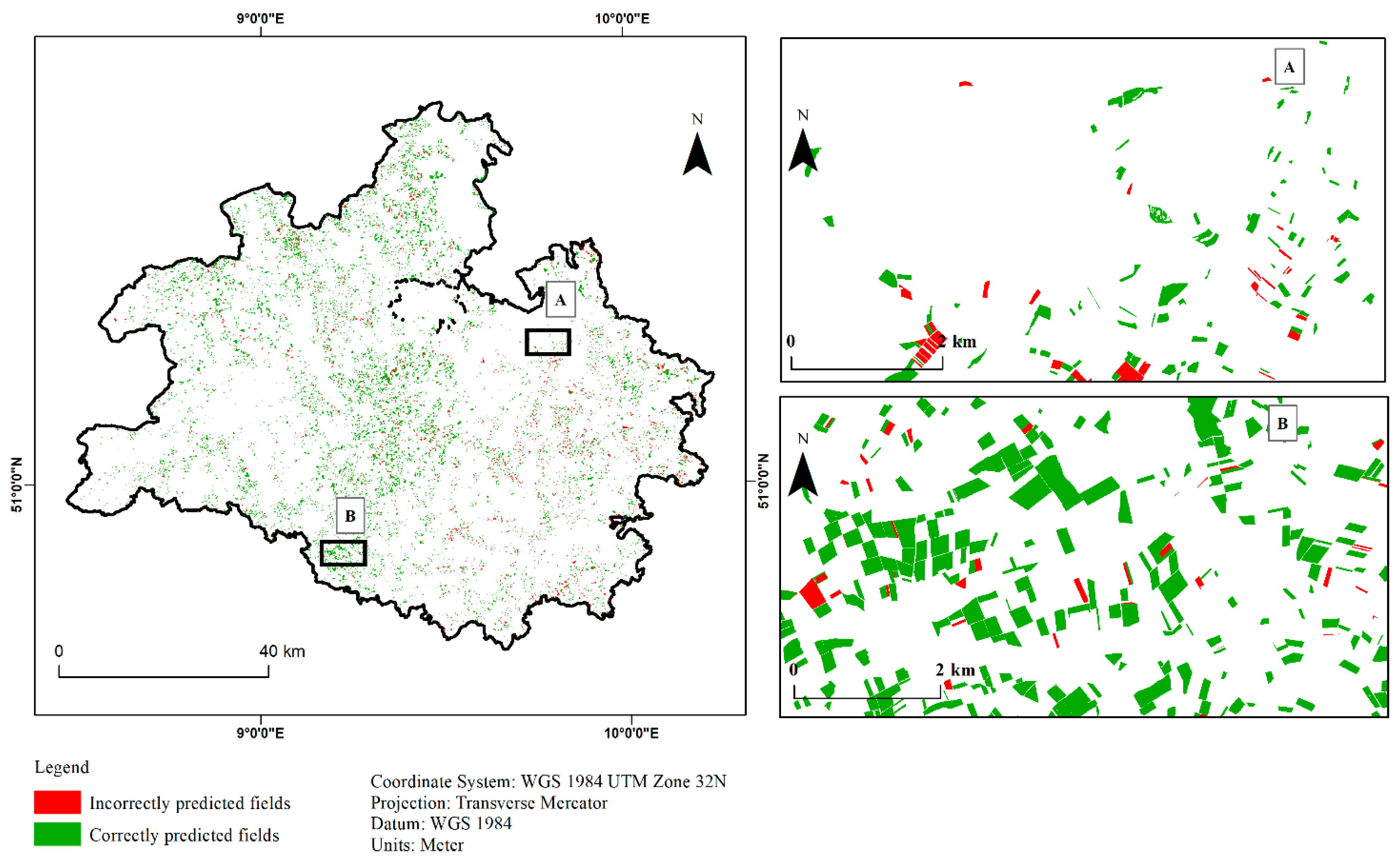
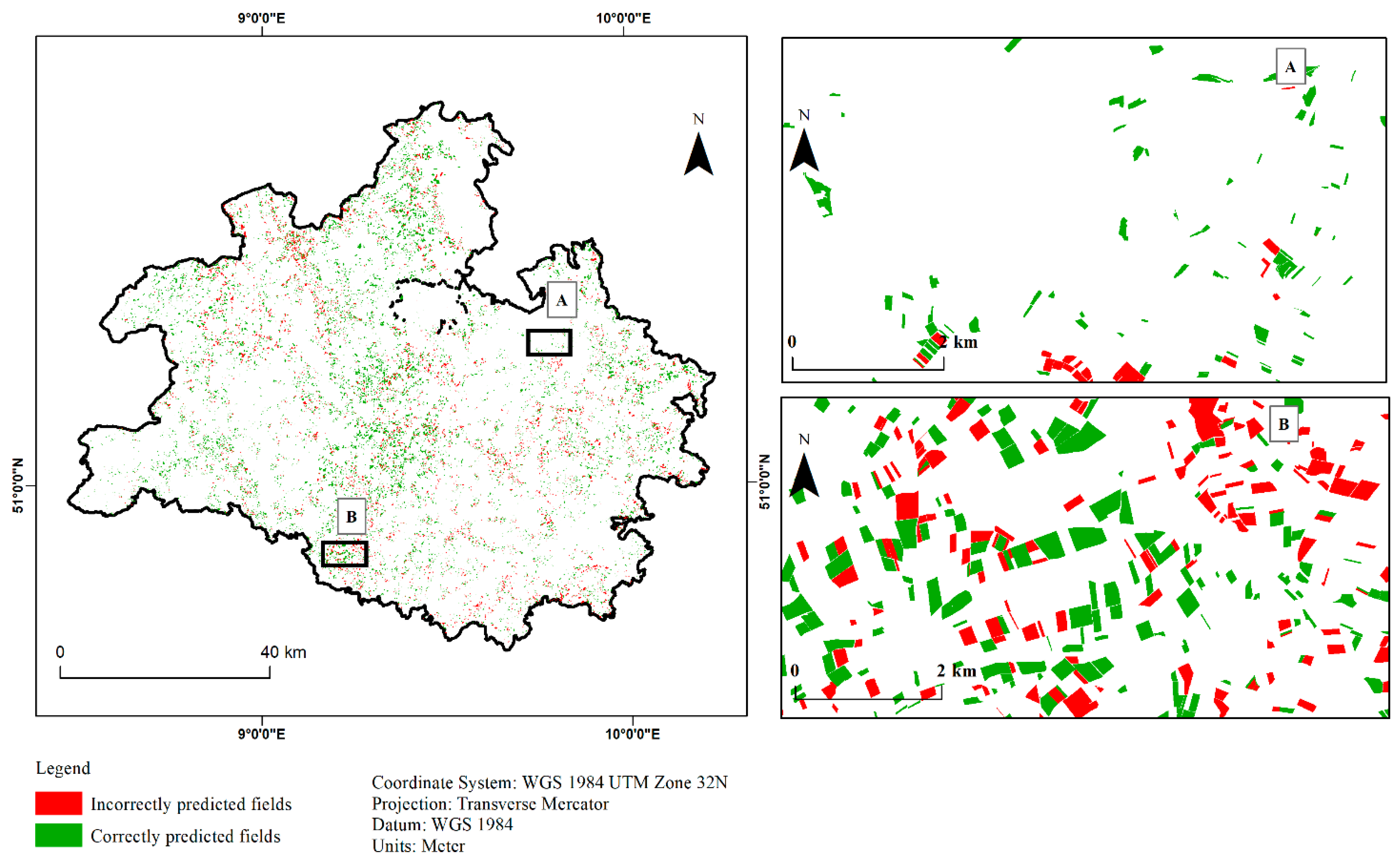
3.3. Classified Maps Based on Best Modelling Method

Since MY models proved to be the best modelling approach, their capability to create accurate crop-type maps are exhibited in Figure 8 for 2015, which corresponds to an OA of 86.1% (see Appendix A,

Table A6. Confusion matrix of the classified map of 2015 using the multiple-year model. The shaded diagonals represent the number of correctly predicted crops. GL = Grassland, MZ = Maize, SC = Summer crops, WC = Winter crops, UA = User accuracy, PA = Producer accuracy, EC = Error of commission, EO = Error of omission and OA = Overall accuracy.

		Reference
		GL	MZ	SC	WC	Total	UA (%)	CE (%)
Prediction	GL	10,313	461	592	1163	12,529	82.31	17.69
	MZ	183	8111	891	69	9254	87.65	12.35
	SC	305	296	9943	1134	11,678	85.14	14.86
	WC	199	53	464	7634	8350	91.43	8.57
	Total	11,000	8921	11,890	10,000
	PA (%)	93.75	90.92	83.62	76.34
	OE (%)	6.25	9.08	16.38	23.66
	OA (%)	86.1

for a confusion matrix). The map was derived with model 6 (Figure 4B), which is an MY model developed based on information from 2005, 2007, 2009, 2010, and 2011. On closer examination, regions at higher altitudes with less favourable growth conditions, which are dominated by grasslands (Figure 8A), can be clearly distinguished from fertile areas, where a multitude of arable crops is grown and where grassland is only interspersed. Moreover, the spatial distribution and patterns of crops, the shape, and edges of fields can clearly be observed. The so-called ‘salt and pepper’ effects, that characterize most land-cover maps at a pixel base were not experienced with the maps produced in this research, which may be a result of the fact that our models were calibrated with the mean spectral information at field scale based on the IACS field polygons. Maps of the remaining years and their respective confusion matrices are shown in the Appendix A, that is, Figure A1, Figure A2, Figure A3, Figure A4 and Figure A5 and

Table A1. Confusion matrix of the classified map of 2005 using the multiple-year model. The shaded diagonals represent the number of correctly predicted crops. GL = Grassland, MZ = Maize, SC = Summer crops, WC = Winter crops, UA = User accuracy, PA = Producer accuracy, EC = Error of commission, EO = Error of omission and OA = Overall accuracy.

		Reference
		GL	MZ	SC	WC	Total	UA (%)	CE (%)
Prediction	GL	4339	137	270	214	4960	87.48	12.52
	MZ	292	4527	442	33	5294	85.51	14.49
	SC	264	229	3792	1099	5384	70.43	29.57
	WC	105	48	496	3654	4303	84.92	15.08
	Total	5000	4941	5000	5000
	PA (%)	86.78	91.62	75.84	73.08
	OE (%)	13.22	8.38	24.16	26.92
	OA (%)	81.8

,

Table A2. Confusion matrix of the classified map of 2007 using the multiple-year model. The shaded diagonals represent the number of correctly predicted crops. GL = Grassland, MZ = Maize, SC = Summer crops, WC = Winter crops, UA = User accuracy, PA = Producer accuracy, EC = Error of commission, EO = Error of omission and OA = Overall accuracy.

		Reference
		GL	MZ	SC	WC	Total	UA (%)	CE (%)
Prediction	GL	4380	203	316	156	5055	86.65	13.35
	MZ	158	3738	463	38	4397	85.01	14.99
	SC	68	358	3384	154	3964	85.37	14.63
	WC	394	90	837	4652	5973	77.88	22.12
	Total	5000	4389	5000	5000
	PA (%)	87.60	85.17	67.68	93.04
	OE (%)	12.40	14.83	32.32	6.96
	OA (%)	83.32

,

Table A3. Confusion matrix of the classified map of 2009 using the multiple-year model. The shaded diagonals represent the number of correctly predicted crops. GL = Grassland, MZ = Maize, SC = Summer crops, WC = Winter crops, UA = User accuracy, PA = Producer accuracy, EC = Error of commission, EO = Error of omission and OA = Overall accuracy.

			Reference
		GL	MZ	SC	WC	Total	UA (%)	CE (%)
Prediction	GL	4185	986	430	175	5776	72.45	27.55
	MZ	166	4070	394	26	4656	87.41	12.59
	SC	345	889	3347	748	5329	62.81	37.19
	WC	304	531	1743	4051	6629	61.11	38.89
	Total	5000	6476	5914	5000
	PA (%)	83.70	62.85	56.59	81.02
	OE (%)	16.30	37.15	43.41	18.98
	OA (%)	69.91

,

Table A4. Confusion matrix of the classified map of 2010 using the multiple-year model. The shaded diagonals represent the number of correctly predicted crops. GL = Grassland, MZ = Maize, SC = Summer crops, WC = Winter crops, UA = User accuracy, PA = Producer accuracy, EC = Error of commission, EO = Error of omission and OA = Overall accuracy.

		Reference
		GL	MZ	SC	WC	Total	UA (%)	CE (%)
Prediction	GL	4262	376	179	91	4908	86.84	13.16
	MZ	172	4990	956	185	6303	79.17	20.83
	SC	238	1830	4388	827	7283	60.25	39.75
	WC	328	171	307	3897	4703	82.86	17.14
	Total	5000	7367	5830	5000
	PA (%)	85.24	67.73	75.27	77.94
	OE (%)	14.76	32.27	24.73	22.06
	OA (%)	75.6

and

Table A5. Confusion matrix of the classified map of 2011 using the multiple-year model. The shaded diagonals represent the number of correctly predicted crops. GL = Grassland, MZ = Maize, SC = Summer crops, WC = Winter crops, UA = User accuracy, PA = Producer accuracy, EC = Error of commission, EO = Error of omission and OA = Overall accuracy.

		Reference
		GL	MZ	SC	WC	Total	UA (%)	CE (%)
Prediction	GL	4493	209	264	460	5426	82.81	17.19
	MZ	141	3427	732	151	4451	76.99	23.01
	SC	108	4073	4644	363	9188	50.54	49.46
	WC	258	507	872	4026	5663	71.09	28.91
	Total	5000	8216	6512	5000
	PA (%)	89.86	41.71	71.31	80.52
	OE (%)	10.14	58.29	28.69	19.48
	OA (%)	67.09

, respectively.

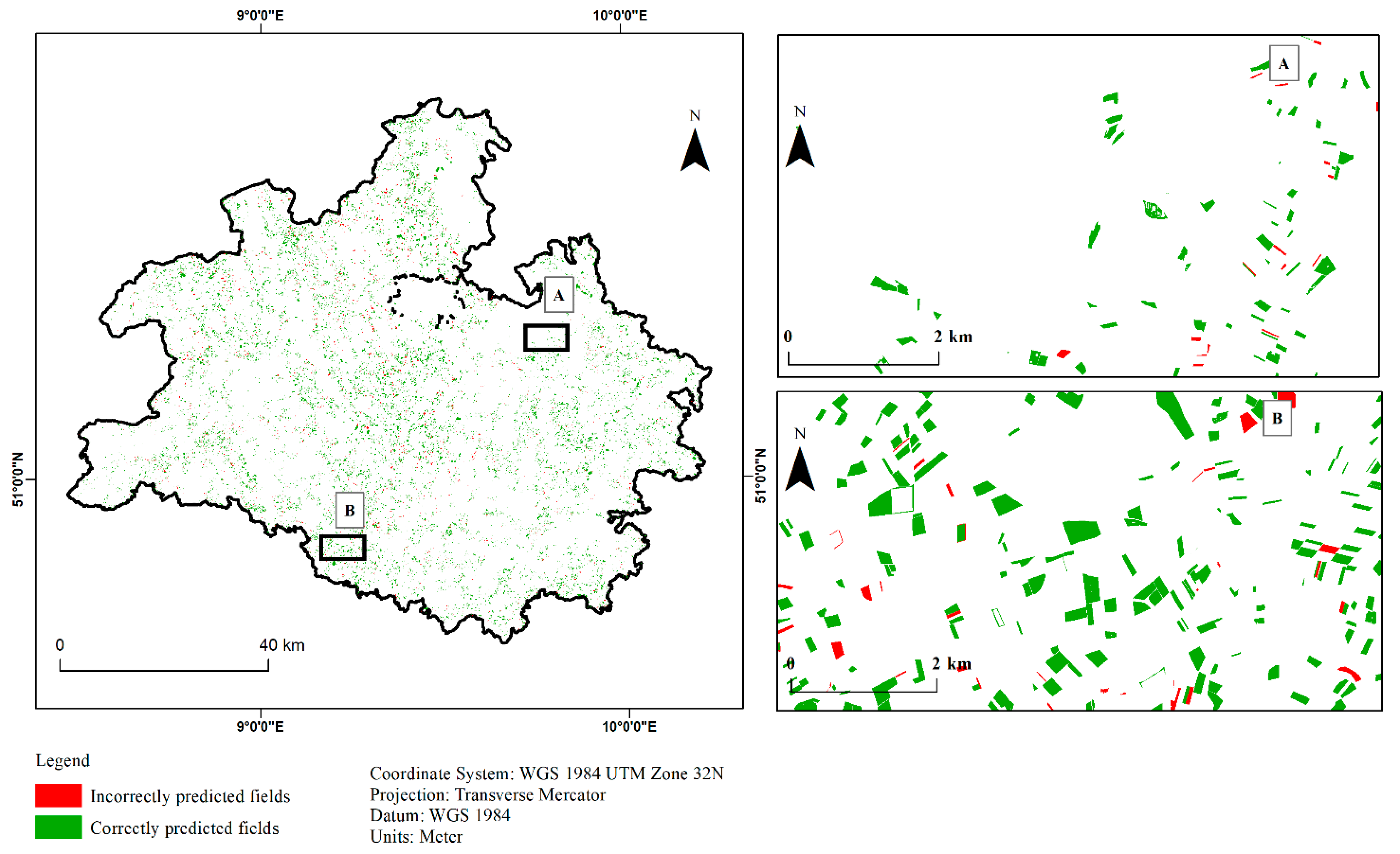
3.4. Relationship between Model Accuracy and Field Size

An increase in mean accuracy from 74% to 87% was observed as the field size increased (i.e., 1.5–9 ha) (Figure 9). Furthermore, a slight decrease in the mean accuracy from 87% to 85% of crop type prediction was seen with increasing field size from 9 ha to 12 ha. As the field size increased further to 13.5 ha, a slight increase in accuracy was observed (from 85% to 88%). However, a marginal reduction to 87% accuracy was observed as the field size increased further. The consistent and marginal rise and fall in accuracy with increasing field sizes indicate that crop type prediction by MY models is independent of field size. But it is important to state that the majority of fields (> 60%) belong to the smallest field category (1.5 ha). The accuracy maps of the MY models can be seen in Figure 10 and the rest in the Appendix A (Figure A6, Figure A7, Figure A8, Figure A9 and Figure A10)

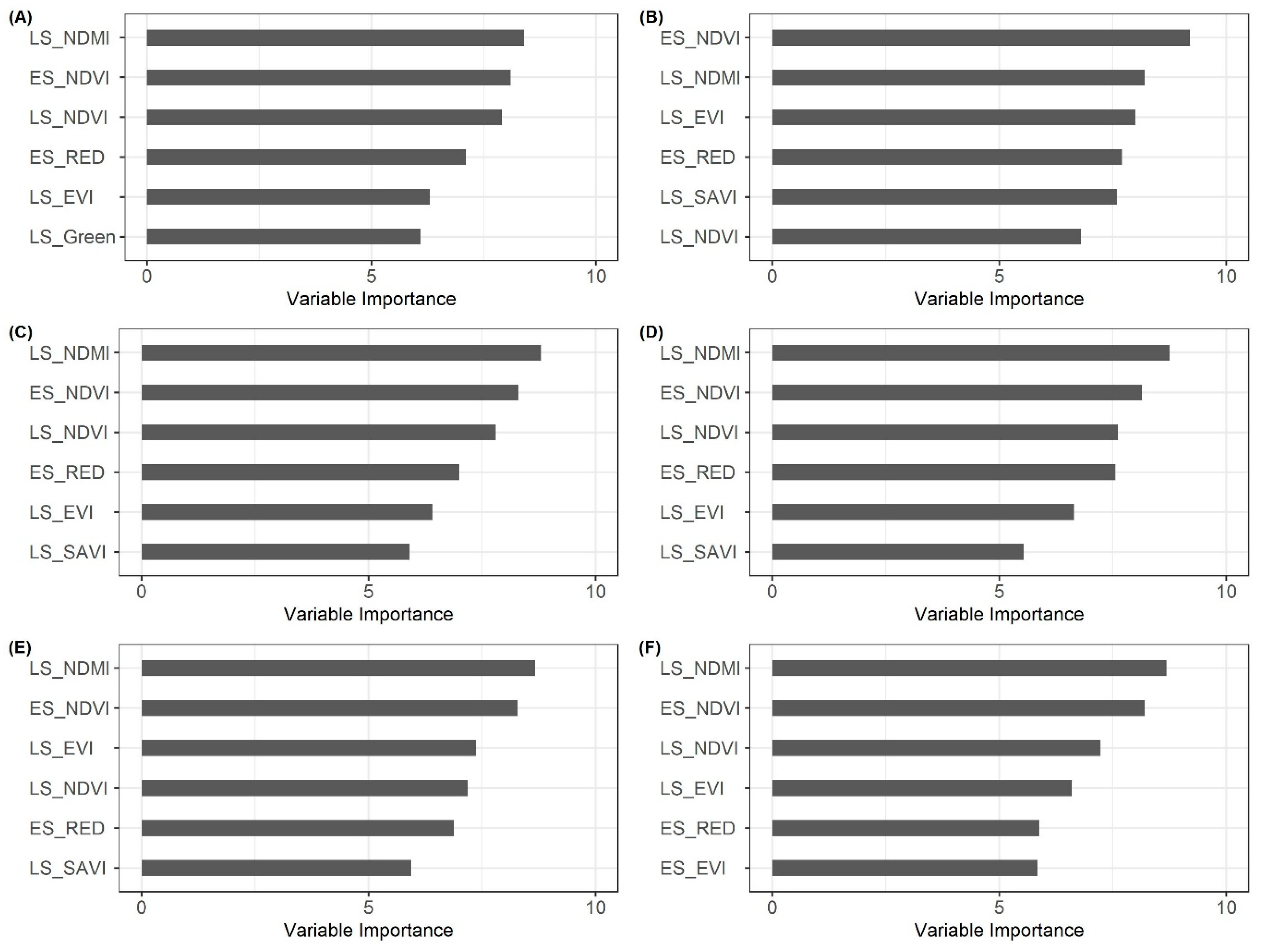
3.5. Importance of Predictor Variables

One of the strengths of RF models is the ability to measure and assess the contribution of each predictor variable used. Figure 11 presents the importance values of the first 6 most important input variables used in the MY models. Late summer (LS) NDMI was the first most important predictor variable in most models, and only in one instance the means of early summer (ES) NDVI was ranked first (Figure 11B). Another predictor that seemed to be important across models was the early summer NDVI as shown in Figure 11A,C–F. The contribution of VIs in the prediction of crops was much stronger than the individual bands. Red and green bands are the only bands that appeared among the first six important predictors, with red being the dominant one across all models.

4. Discussion

Crop type mapping in large agricultural landscapes is challenged by the daunting task of periodic training data collection. The traditional satellite-based mapping approach of using reference data from the same year impedes mapping specifically in periods where reference data is not available. The IACS data, which is a field-based crop type data presents reliable reference datasets to deal with the problem of frequent training data collection for satellite-based crop type mapping through the development of a generalized model. The issue of generalized classifiers has been raised and exploited in a few agricultural mapping studies, but less focus was put on specific crop type mapping. Thus, this study aimed at assessing the efficacy of IACS data to be used as reference data for the development of generalized SY and MY crop type models to predict grassland, maize, summer and winter crops as land-cover categories.

The accuracies achieved in our study are similar to the work of [8], where corn and soybeans were predicted based on spectral characteristics using the single-year modelling approach. While our study considers four different crop types with an acceptable average UA and PA for grassland across years (>80%), maize, summer and winter crops were predicted at somewhat lower accuracies. That means that despite the somewhat low performance of SY models in predicting the other crop types, it is able to predict grassland with an acceptable level of accuracy across years.

The overall accuracy of the SY calibration method employed in our study is rather low compared to the traditional method, where calibration and testing data are from the same year. Probable reasons may be different growing dates of the crops in different years, inter-annual differences in climate, image acquisition time as well as variation in image quality between years, as was also suggested by Laborte et al., [58] and Zhong et al., [8]. The performance of MY models in predicting crop types showed higher robustness across years than the SY calibration approach. An average increment of 6% in OA (i.e., 77.3%) was achieved by MY models across years. A similar OA of 73.1% was achieved by Massey et al., [37] when an MY calibrated model was used to predict crop types from MODIS data for an independent year. The higher robustness of MY models might be attributable to the fact that, through the use of spectral information from different years, the interannual climate variability as well as variations in image quality from different years, are reduced to a certain degree [8,58]. Thus, these factors make them generic with high prediction accuracies when applied to predict crops from data not seen by the model. Additionally, MY calibration compensates for the phenological differences of crops among years through the inclusion of many phenological situations using multiple data from different years. This makes MY models more efficient and generalized for satellite-based crop type classification when training data is not available for a period of interest.

The prediction of crops from the spectral-temporal profiles of satellite images can heavily depend on the time and quality of the images used [10,58]. Occasionally, a compromise has to be made between the quality and time of images in the same growing season, which may ultimately have the consequence that not all years will have high accuracies when data from multiple years are used [8]. In this study, for example, the 2009 and 2011 seasons comprised of very late September and October images (Table 2) due to the lack of earlier images. However, in the study area, maize fields are harvested as late as the end of September or early October, whereas summer crops are harvested much earlier to give way for winter crops, which might have developed one or two leaves at this time. Such sources of variation might explain the somewhat lower accuracies of 2009 and 2011 data as compared to the other years.

The data on the assessment of the spectral predictors used in the MY models indicates a paramount contribution of VIs in the prediction of crops as compared to the individual bands. A similar conclusion was drawn by Fletcher [59] in the discrimination of soybean and three weed species. The highest contribution of VIs in the prediction of the crops was expected since their calculation involved two or more bands and as a result, used the unique spectral characteristics of the individual bands to produce a single layer which captured the different phenological dynamics among the crops. Vegetation indices, which are based on SWIR and NIR spectral bands, are known for their contributions to plant separation [59]. Therefore, despite the contributions of the other predictor variables, the late summer NDMI is ranked as the topmost dominant predictor variables for almost all years, followed by early summer NDVI. NDMI uses a normalized ratio of the difference and sum of NIR and SWIR and is known to be sensitive to changes in water content of vegetations canopies [56]. It can, therefore, be inferred that the differences among the four crop types are better captured by the content of moisture in their leaf canopies during late summer.

The subject of object size and prediction accuracy is very crucial in the mapping of agricultural areas [39]. Our results suggest that the prediction of a particular crop type does not necessarily depend on the corresponding size of the field. It was expected that the prediction of bigger fields may be easier than with smaller fields, but the results do not confirm that. The biggest crop field category (≥15 ha) achieved a prediction accuracy of 88%, nonetheless, comparatively smaller field sizes (9 ha) also achieved the same accuracy. Thus, the present study does not support the conclusions of Castilla et al., [41], that the possibility of correct classification of land-cover type decreases with decreasing object size. The reason may be that Castilla et al., [41] employed a segmentation method, which is dependent on the land cover size, whereas the present study used the exact field polygons declared by farmers in the study area as objects for the prediction of the crop types. However, since the present study area is dominated by smaller fields with very few large fields, future research is required to further investigate the relationship between field size and accuracy of crop types prediction in agricultural areas with a relatively even distribution of field sizes.

The uniqueness of this study compared to other studies of generalized classifiers for cropland mapping is the field-based approach employed. This approach deals with some of the challenges associated with the widely used methods. The issue of segmentation scale selection of the other object-based classification [21] is avoided. Moreover, the ‘salt and pepper’ effects that characterize the pixel-based prediction of land-cover types are equally averted in this study. Hence, our MY modelling approach can be used to map past and present crop types which may be necessary to ascertain the impacts of any agricultural activity (e.g., biogas production) heavily dependent on croplands.

Finally, the hypothesis that IACS data can be used to calibrate models for the prediction of crop types from a satellite image differing from the calibration year has been proven through a field-based SY and MY calibration approach. However, Cai et al., [60] stated that increasing the calibration years to a maximum of 10 years can further increase accuracy. Therefore, our five-year MY models could be improved further by incorporating more years of spectral information, as more satellite data (Sentinel and EnMap) become available in the future.

5. Conclusions

For the first time, this study used a field-based approach to test the usefulness of IACS data in calibrating an RF-based model to predict crop types from satellite images, that are not from the same year as the calibration year. Thus, two modelling methods called SY (i.e., using spectral data from a single year) and MY calibration (i.e., using spectral data from multiple years) were tested in the discrimination of grassland, maize, summer and winter crops.

The results depict a superior performance of the MY approach as compared to SY model. The MY approach included a larger range of inter-annual variability in image quality, climate, and growing dates of crops from different years, thus, contributing to its robustness in predicting crop type from satellite images of different years. The approach employed in this work, unlike other object-based methods, is not dependent on field size. It is, therefore, recommended to use the field-based MY calibration approach for practical crop type mapping, particularly when reference data for the mapping year is not available. This method is useful for practical reasons and can be used to map past and present croplands for comparative analysis. However, the inclusion of soil data and phenological metrics as predictors of MY model may have a potential for future research. This might help improve performance and provide an opportunity for more specific crop type mapping, rather than generic crops like summer and winter crops as used in this study. A combination of data from different satellites like Sentinel or upcoming satellites like EnMap or HyspIRI might further improve the MY modelling approach due to higher revisiting time and thus a denser time series

References

1. Tilman, D.; Balzer, C.; Hill, J.; Befort, B.L. Global food demand and the sustainable intensification of agriculture. Proc. Natl. Acad. Sci. USA 2011, 108, 20260–20264. [Google Scholar] [CrossRef] [PubMed] [Green Version]
2. Nagy, A.; Fehér, J.; Tamás, J. Wheat and maize yield forecasting for the Tisza river catchment using MODIS NDVI time series and reported crop statistics. Comput. Electron. Agric. 2018, 151, 41–49. [Google Scholar] [CrossRef]
3. See, L.; Fritz, S.; You, L.; Ramankutty, N.; Herrero, M.; Justice, C.; Becker-Reshef, I.; Thornton, P.; Erb, K.; Gong, P.; et al. Improved global cropland data as an essential ingredient for food security. Glob. Food Secur. 2015, 4, 37–45. [Google Scholar] [CrossRef]
4. Gumma, M.K.; Thenkabail, P.S.; Teluguntla, P.; Rao, M.N.; Mohammed, I.A.; Whitbread, A.M. Mapping rice-fallow cropland areas for short-season grain legumes intensification in South Asia using MODIS 250 m time-series data. Int. J. Digit. Earth 2016, 9, 981–1003. [Google Scholar] [CrossRef] [Green Version]
5. Funk, C.C.; Brown, M.E. Declining global per capita agricultural production and warming oceans threaten food security. Food Secur. 2009, 1, 271–289. [Google Scholar] [CrossRef]
6. Pérez-Hoyos, A.; Rembold, F.; Kerdiles, H.; Gallego, J. Comparison of global land cover datasets for cropland monitoring. Remote Sens. 2017, 9, 1118. [Google Scholar] [CrossRef]
7. Tatsumi, K.; Yamashiki, Y.; Canales Torres, M.A.; Taipe, C.L.R. Crop classification of upland fields using Random forest of time-series Landsat 7 ETM+ data. Comput. Electron. Agric. 2015, 115, 171–179. [Google Scholar] [CrossRef]
8. Zhong, L.; Gong, P.; Biging, G.S. Efficient corn and soybean mapping with temporal extendability: A multi-year experiment using Landsat imagery. Remote Sens. Environ. 2014, 140, 1–13. [Google Scholar] [CrossRef]
9. Castillejo-González, I. Mapping of Olive Trees Using Pansharpened QuickBird Images: An Evaluation of Pixel- and Object-Based Analyses. Agronomy 2018, 8, 288. [Google Scholar] [CrossRef]
10. Foerster, S.; Kaden, K.; Foerster, M.; Itzerott, S. Crop type mapping using spectral-temporal profiles and phenological information. Comput. Electron. Agric. 2012, 89, 30–40. [Google Scholar] [CrossRef]
11. Moeckel, T.; Dayananda, S.; Nidamanuri, R.R.; Nautiyal, S.; Hanumaiah, N.; Buerkert, A.; Wachendorf, M. Estimation of vegetable crop parameter by multi-temporal UAV-borne images. Remote Sens. 2018, 10, 805. [Google Scholar] [CrossRef]
12. Wu, B.; Meng, J.; Li, Q.; Yan, N.; Du, X.; Zhang, M. Remote sensing-based global crop monitoring: Experiences with China’s CropWatch system. Int. J. Digit. Earth 2014, 7, 113–137. [Google Scholar] [CrossRef]
13. Pittman, K.; Hansen, M.C.; Becker-Reshef, I.; Potapov, P.V.; Justice, C.O. Estimating global cropland extent with multi-year MODIS data. Remote Sens. 2010, 2, 1844–1863. [Google Scholar] [CrossRef]
14. Waldhoff, G.; Lussem, U.; Bareth, G. Multi-Data Approach for remote sensing-based regional crop rotation mapping: A case study for the Rur catchment, Germany. Int. J. Appl. Earth Obs. Geoinf. 2017, 61, 55–69. [Google Scholar] [CrossRef]
15. Habyarimana, E.; Piccard, I.; Catellani, M.; De Franceschi, P.; Dall’Agata, M. Towards Predictive Modeling of Sorghum Biomass Yields Using Fraction of Absorbed Photosynthetically Active Radiation Derived from Sentinel-2 Satellite Imagery and Supervised Machine Learning Techniques. Agronomy 2019, 9, 203. [Google Scholar] [CrossRef]
16. Liu, J.; Feng, Q.; Gong, J.; Zhou, J.; Liang, J.; Li, Y. Winter wheat mapping using a random forest classifier combined with multi-temporal and multi-sensor data. Int. J. Digit. Earth 2018, 11, 783–802. [Google Scholar] [CrossRef]
17. Maxwell, S.K.; Nuckols, J.R.; Ward, M.H.; Hoffer, R.M. An automated approach to mapping corn from Landsat imagery. Comput. Electron. Agric. 2004, 43, 43–54. [Google Scholar] [CrossRef]
18. Yin, H.; Prishchepov, A.V.; Kuemmerle, T.; Bleyhl, B.; Buchner, J.; Radeloff, V.C. Mapping agricultural land abandonment from spatial and temporal segmentation of Landsat time series. Remote Sens. Environ. 2018, 210, 12–24. [Google Scholar] [CrossRef]
19. Zheng, B.; Myint, S.W.; Thenkabail, P.S.; Aggarwal, R.M. A support vector machine to identify irrigated crop types using time-series Landsat NDVI data. Int. J. Appl. Earth Obs. Geoinf. 2015, 34, 103–112. [Google Scholar] [CrossRef]
20. Waldner, F.; Hansen, M.C.; Potapov, P.V.; Löw, F.; Newby, T.; Ferreira, S.; Defourny, P. National-scale cropland mapping based on spectral-temporal features and outdated land cover information. PLoS ONE 2017, 12, e0181911. [Google Scholar] [CrossRef]
21. Phiri, D.; Morgenroth, J. Developments in Landsat land cover classification methods: A review. Remote Sens. 2017, 9, 967. [Google Scholar] [CrossRef]
22. Liu, D.; Xia, F. Assessing object-based classification: Advantages and limitations. Remote Sens. Lett. 2010, 1, 187–194. [Google Scholar] [CrossRef]
23. Chen, D.; Stow, D. The Effect of Training Strategies on Supervised Classification at Different Spatial Resolutions. Photogramm. Eng. Remote Sens. 2002, 68, 1155–1162. [Google Scholar]
24. Li, Q.; Wang, C.; Zhang, B.; Lu, L. Object-based crop classification with Landsat-MODIS enhanced time-series data. Remote Sens. 2015, 7, 16091–16107. [Google Scholar] [CrossRef]
25. Zhu, L.; Radeloff, V.C.; Ives, A.R. Improving the mapping of crop types in the Midwestern U.S. by fusing Landsat and MODIS satellite data. Int. J. Appl. Earth Obs. Geoinf. 2017, 58, 1–11. [Google Scholar] [CrossRef]
26. Chen, Y.; Lu, D.; Moran, E.; Batistella, M.; Dutra, L.V.; Sanches, I.D.; da Silva, R.F.B.; Huang, J.; Luiz, A.J.B.; de Oliveira, M.A.F. Mapping croplands, cropping patterns, and crop types using MODIS time-series data. Int. J. Appl. Earth Obs. Geoinf. 2018, 69, 133–147. [Google Scholar] [CrossRef]
27. Foody, G.M.; Mathur, A.; Sanchez-Hernandez, C.; Boyd, D.S. Training set size requirements for the classification of a specific class. Remote Sens. Environ. 2006, 104, 1–14. [Google Scholar] [CrossRef]
28. Botkin, D.B.; Estes, J.E.; MacDonald, R.M.; Wilson, M.V. Studying the Earth’s Vegetation from Space. Bioscience 1984, 34, 508–514. [Google Scholar] [CrossRef]
29. Sonobe, R.; Yamaya, Y.; Tani, H.; Wang, X.; Kobayashi, N.; Mochizuki, K.I. Mapping crop cover using multi-temporal landsat 8 oli imagery. Int. J. Remote Sens. 2017, 38, 4348–4361. [Google Scholar] [CrossRef]
30. Vuolo, F.; Neuwirth, M.; Immitzer, M.; Atzberger, C.; Ng, W.-T. How much does multi-temporal Sentinel-2 data improve crop type classification? Int. J. Appl. Earth Obs. Geoinf. 2018, 72, 122–130. [Google Scholar] [CrossRef]
31. Zhao, Y.; Feng, D.; Yu, L.; Wang, X.; Chen, Y.; Bai, Y.; Hernández, H.J.; Galleguillos, M.; Estades, C.; Biging, G.S.; et al. Detailed dynamic land cover mapping of Chile: Accuracy improvement by integrating multi-temporal data. Remote Sens. Environ. 2016, 183, 170–185. [Google Scholar] [CrossRef]
32. Xiao, X.; Boles, S.; Liu, J.; Zhuang, D.; Frolking, S.; Li, C.; Salas, W.; Moore, B. Mapping paddy rice agriculture in southern China using multi-temporal MODIS images. Remote Sens. Environ. 2005, 95, 480–492. [Google Scholar] [CrossRef]
33. Manfron, G.; Delmotte, S.; Busetto, L.; Hossard, L.; Ranghetti, L.; Brivio, P.A.; Boschetti, M. Estimating inter-annual variability in winter wheat sowing dates from satellite time series in Camargue, France. Int. J. Appl. Earth Obs. Geoinf. 2017, 57, 190–201. [Google Scholar] [CrossRef]
34. Huete, A.; Didan, K.; Miura, T.; Rodriguez, E.P.; Gao, X.; Ferreira, L.G. Overview of the radiometric and biophysical performance of the MODIS vegetation indices. Remote Sens. Environ. 2002, 83, 195–213. [Google Scholar] [CrossRef]
35. Bill, R.; Nash, E.; Grenzdörffer, G. Integrated Administration and Control System. In Springer Handbook of Geographic Information System; Kresse, W., Danko, D.M., Eds.; Springer: Berlin, Germany, 2012; pp. 801–803. ISBN 978-3-540-72678-4. [Google Scholar]
36. Boryan, C.; Yang, Z.; Mueller, R.; Craig, M. Monitoring US agriculture: The US department of agriculture, national agricultural statistics service, cropland data layer program. Geocarto Int. 2011, 26, 341–358. [Google Scholar] [CrossRef]
37. Massey, R.; Sankey, T.T.; Congalton, R.G.; Yadav, K.; Thenkabail, P.S.; Ozdogan, M.; Sánchez Meador, A.J. MODIS phenology-derived, multi-year distribution of conterminous U.S. crop types. Remote Sens. Environ. 2017, 198, 490–503. [Google Scholar] [CrossRef]
38. Griffiths, P.; Nendel, C.; Hostert, P. Intra-annual reflectance composites from Sentinel-2 and Landsat for national-scale crop and land cover mapping. Remote Sens. Environ. 2019, 220, 135–151. [Google Scholar] [CrossRef]
39. Ma, L.; Li, M.; Ma, X.; Cheng, L.; Du, P.; Liu, Y. ISPRS Journal of Photogrammetry and Remote Sensing A review of supervised object-based land-cover image classification. ISPRS J. Photogramm. Remote Sens. 2017, 130, 277–293. [Google Scholar] [CrossRef]
40. Blaschke, T.; Hay, G.J.; Kelly, M.; Lang, S.; Hofmann, P.; Addink, E.; Queiroz Feitosa, R.; van der Meer, F.; van der Werff, H.; van Coillie, F.; et al. Geographic Object-Based Image Analysis—Towards a new paradigm. ISPRS J. Photogramm. Remote Sens. 2014, 87, 180–191. [Google Scholar] [CrossRef]
41. Castilla, G.; Hernando, A.; Zhang, C.; McDermid, G.J. The impact of object size on the thematic accuracy of landcover maps. Int. J. Remote Sens. 2014, 35, 1029–1037. [Google Scholar] [CrossRef]
42. Wagner, B. Spatial analysis of loess and loess-like sediments in the Weser-Aller catchment (Lower Saxony and Northern Hesse, NW Germany). Quarernary Sci. J. 2011, 60, 27–46. [Google Scholar] [CrossRef] [Green Version]
43. HLNUG Hessian Agency for Nature Conservation, Environment and Geology. Available online: Atlas.umwelt.hessen.de (accessed on 9 November 2018).
44. USGS Landsat Surface Reflectance Products. Available online: https://earthexplorer.usgs.gov/ (accessed on 24 July 2018).
45. Masek, J.G.; Vermote, E.F.; Saleous, N.E.; Wolfe, R.; Hall, F.G.; Huemmrich, K.F.; Gao, F.; Kutler, J.; Lim, T.K. A landsat surface reflectance dataset for North America, 1990–2000. IEEE Geosci. Remote Sens. Lett. 2006, 3, 68–72. [Google Scholar] [CrossRef]
46. Vermote, E.; Justice, C.; Claverie, M.; Franch, B. Preliminary analysis of the performance of the Landsat 8/OLI land surface reflectance product. Remote Sens. Environ. 2016, 185, 46–56. [Google Scholar] [CrossRef]
47. Flood, N. Continuity of reflectance data between landsat-7 ETM+ and landsat-8 OLI, for both top-of-atmosphere and surface reflectance: A study in the australian landscape. Remote Sens. 2014, 6, 7952–7970. [Google Scholar] [CrossRef]
48. Li, P.; Jiang, L.; Feng, Z. Cross-comparison of vegetation indices derived from landsat-7 enhanced thematic mapper plus (ETM+) and landsat-8 operational land imager (OLI) sensors. Remote Sens. 2014, 6, 310–329. [Google Scholar] [CrossRef]
49. USGS Landsat Science Products-Landsat Surface Reflectance. Available online: https://www.usgs.gov/land-resources/nli/landsat/landsat-surface-reflectance?qt-science_support_page_related_con=0#qt-science_support_page_related_con (accessed on 10 May 2019).
50. Hijmans, R.J.; van Etten, J.; Cheng, J.; Mattiuzzi, M.; Sumner, M.; Greenberg, J.A.; Lamigueiro, O.P.; Bevan, A.; Racine, E.B.; Shortridge, A. Package “raster”. R Package 2019, version 2.9-5. 1–60. [Google Scholar]
51. Team, R.D.C. R Development Core Team R. R A Lang. Environ. Stat. Comput. 2015, 1, 409. [Google Scholar]
52. Breiman, L. Random forest. Mach. Learn. 2001, 45, 5–32. [Google Scholar] [CrossRef]
53. Belgiu, M.; Drăgu, L. Random forest in remote sensing: A review of applications and future directions. ISPRS J. Photogramm. Remote Sens. 2016, 114, 24–31. [Google Scholar] [CrossRef]
54. Tucker, C.J. Red and photographic infrared linear combinations for monitoring vegetation. Remote Sens. Environ. 1979, 8, 127–150. [Google Scholar] [CrossRef] [Green Version]
55. Huete, A. A soil-adjusted vegetation index (SAVI). Remote Sens. Environ. 1988, 25, 295–309. [Google Scholar] [CrossRef]
56. Gao, B.C. NDWI-A normalized difference water index for remote sensing of vegetation liquid water from space. Remote Sens. Environ. 1996, 58, 257–266. [Google Scholar] [CrossRef]
57. Liaw, A.; Wiener, M. Classification and Regression by randomForest. R News 2002, 2, 18–22. [Google Scholar]
58. Laborte, A.G.; Maunahan, A.A.; Hijmans, R.J. Spectral Signature Generalization and Expansion Can Improve the Accuracy of Satellite Image Classification. PLoS ONE 2010, 5, e10516. [Google Scholar] [CrossRef] [PubMed]
59. Fletcher, R.S. Using Vegetation Indices as Input into Random Forest for Soybean and Weed Classification. Am. J. Plant Sci. 2016, 07, 2186–2198. [Google Scholar] [CrossRef] [Green Version]
60. Cai, Y.; Guan, K.; Peng, J.; Wang, S.; Seifert, C.; Wardlow, B.; Li, Z. A high-performance and in-season classification system of field-level crop types using time-series Landsat data and a machine learning approach. Remote Sens. Environ. 2018, 210, 35–47. [Google Scholar] [CrossRef]
Figure 1. Map of the study area. (A) shows a map of Germany and the location of the study area, with the boundaries of the Landsat scenes; (B) shows the five districts, where the study was done.
Agronomy 09 00309 g001
Figure 2. Vegetation profiles of the four crops based on enhanced vegetation index (EVI). Early summer = April to May, Late summer = July to October.
Agronomy 09 00309 g002
Figure 3. The workflow of the data analysis. SY-Single-year, MY-Multiple-years, VIs-Vegetation Indices, B-Blue, G-Green, R-Red, NIR-Near Infra-red, SWIR-Shortwave Infra-red, NDVI-Normalized Difference Vegetation Index, EVI-Enhanced Vegetation Index, SAVI-Soil Adjusted Vegetation Index, NDMI-Normalized Difference Moisture Index.
Agronomy 09 00309 g003
Figure 4. An illustration of the two modelling approaches.
Agronomy 09 00309 g004
Figure 5. Characteristics of Integrated Administration and Control System (IACS) data used as reference information for the predictive crop type models.
Agronomy 09 00309 g005
Figure 6. Accuracies of single year models. The mean bars represent average PA and UA, respectively, for each crop across years. Values in brackets represent the average overall accuracies of all models. UA = User accuracy and PA = producer accuracy.
Agronomy 09 00309 g006
Figure 7. Accuracies of multiple-year models. The mean bars represent average producer accuracies (PA) and user accuracy (UA), respectively, for each crop across years. Values in brackets represent the average overall accuracies of all models.
Agronomy 09 00309 g007
Figure 8. A classified map of 2015 resulting from a multiple-year model based on spectral information of 2005, 2007, 2009, 2010 and 2011. ‘A’ and ‘B’ show areas dominated by grassland at higher altitudes and fertile areas dominated by arable crops respectively.
Agronomy 09 00309 g008
Figure 9. The relationship between the accuracy of crop type prediction and field size based on the multiple-year models. The accuracies are mean values for all years, with the last bin representing the average accuracy of all fields ranging 15–34.5 ha. The value on top of each bar represents the number of fields for each field size group.
Agronomy 09 00309 g009
Figure 10. An IACS-based accuracy map of 2015 resulting from a multiple-year model calibrated using spectral data of 2005, 2007, 2009, 2010 and 2011 representing wrongly and correctly predicted fields. ‘A’ and ‘B’ show areas dominated by grassland at higher altitudes and fertile areas dominated by arable crops respectively.
Agronomy 09 00309 g010
Figure 11. The 6 most important predictors used in the multi-year models expressed in decreasing order of importance from the top of the y-axis. Variable importance on the x-axis is expressed as a percentage of Mean Decrease Gini. (AF) are MY models trained by a combination of (2005 + 2007 + 2009 + 2010 + 2011), (2005 + 2007 + 2009 + 2010 + 2015), (2005 + 2007 + 2009 + 2011 + 2015), (2005 + 2007 + 2010 + 2011 + 2015), (2005 + 2009 + 2010 + 2011 + 2015) and (2007 + 2009 + 2010 + 2011 + 2015) respectively. LS = Late summer, ES = Early summer.
Agronomy 09 00309 g011