Field Spectroscopy: A Non-Destructive Technique for Estimating Water Status in Vineyards
 , ,
, ,  and
and 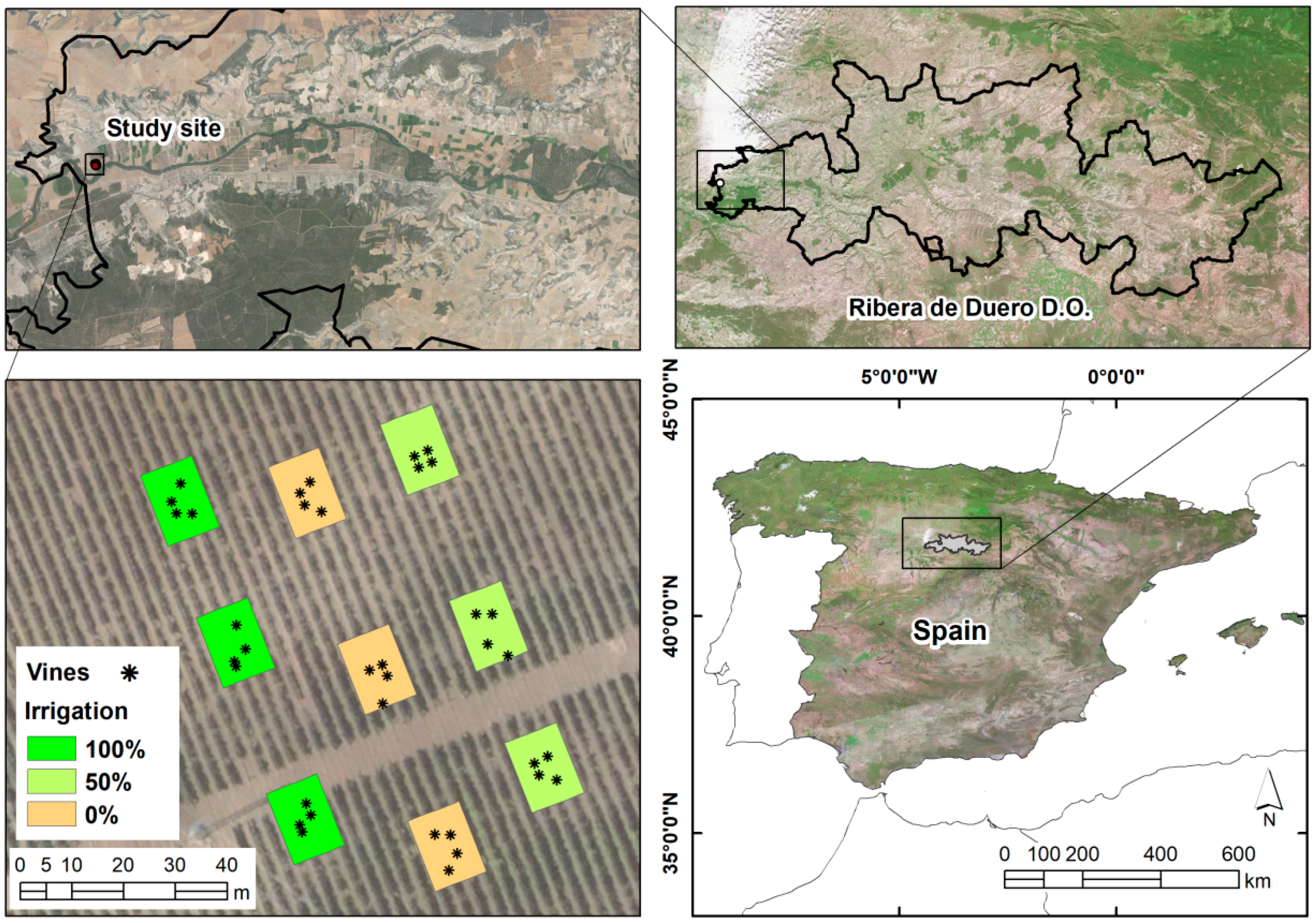
Abstract
:1. Introduction
2. Materials and Methods
2.1. Study Site and Experimental Layout
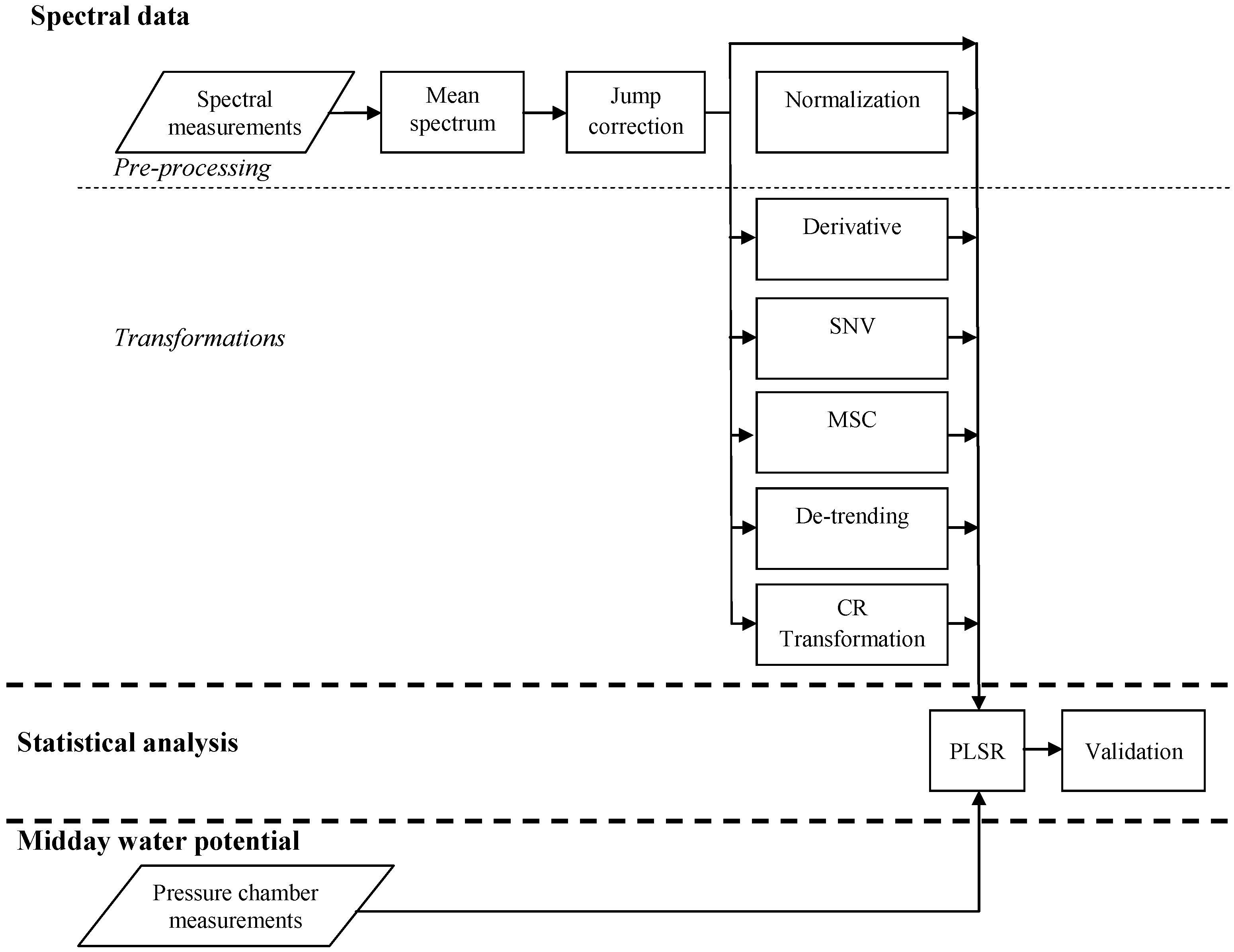
2.2. General Workflow
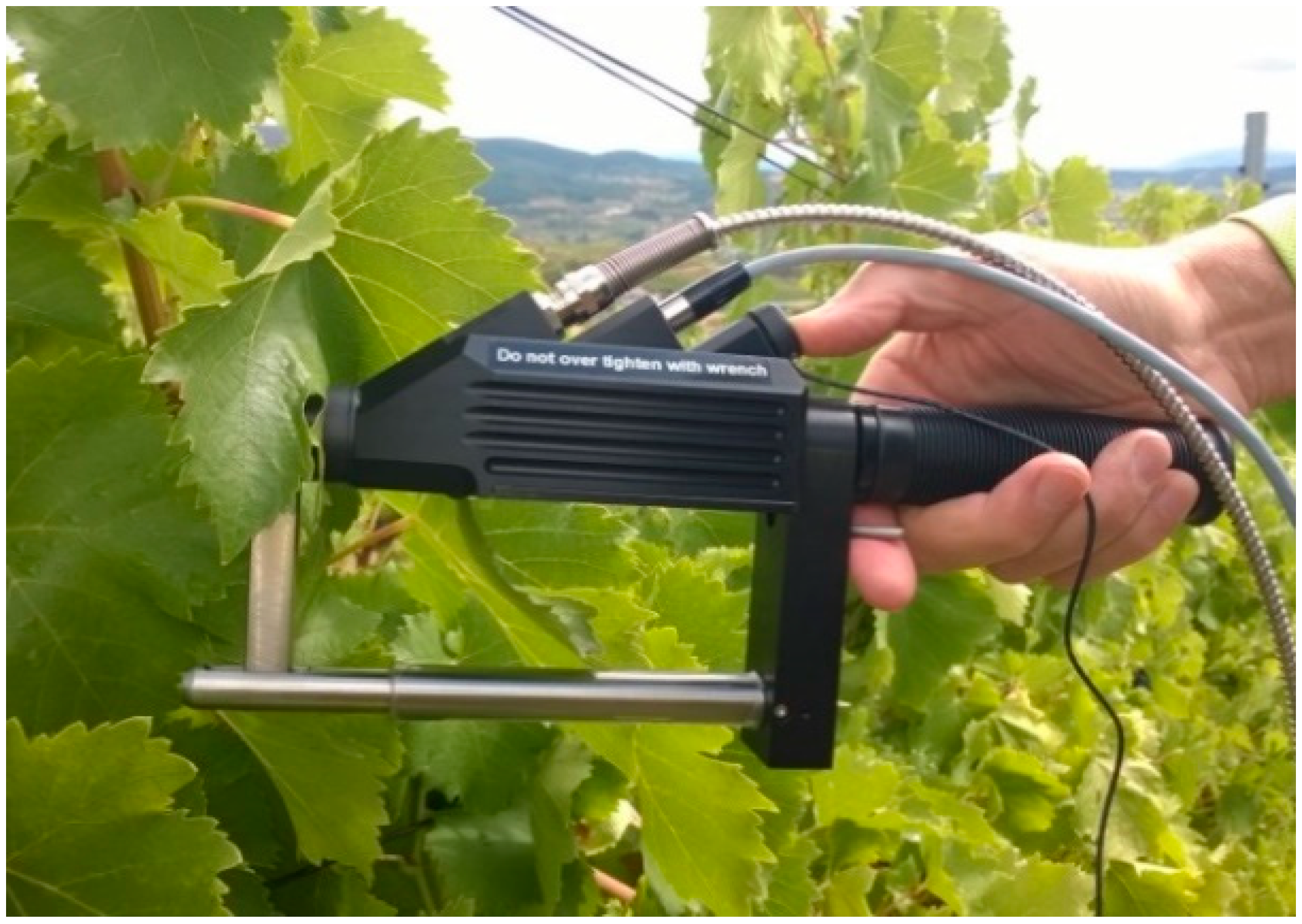
2.3. Leaf Water Status
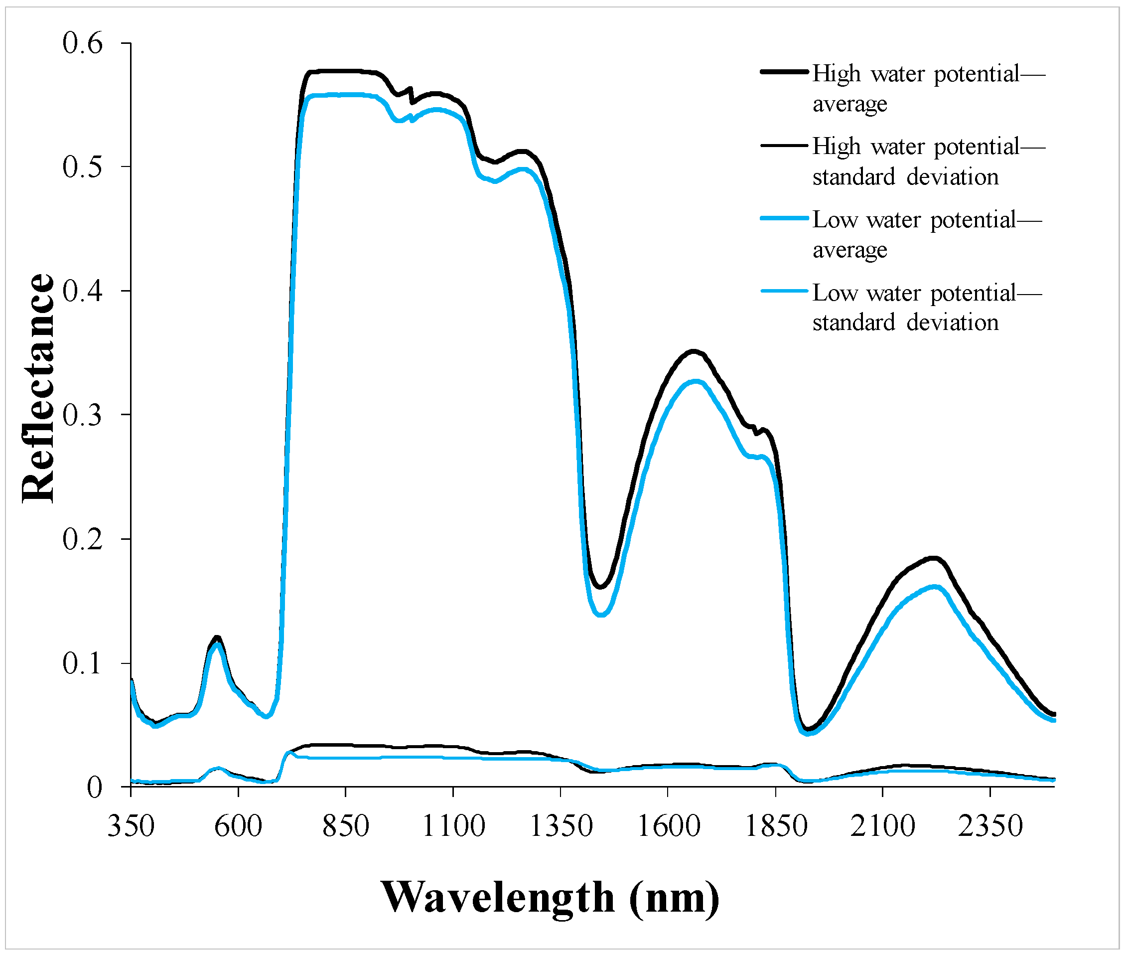
2.4. Spectral Data
2.4.1. Pre-Processing
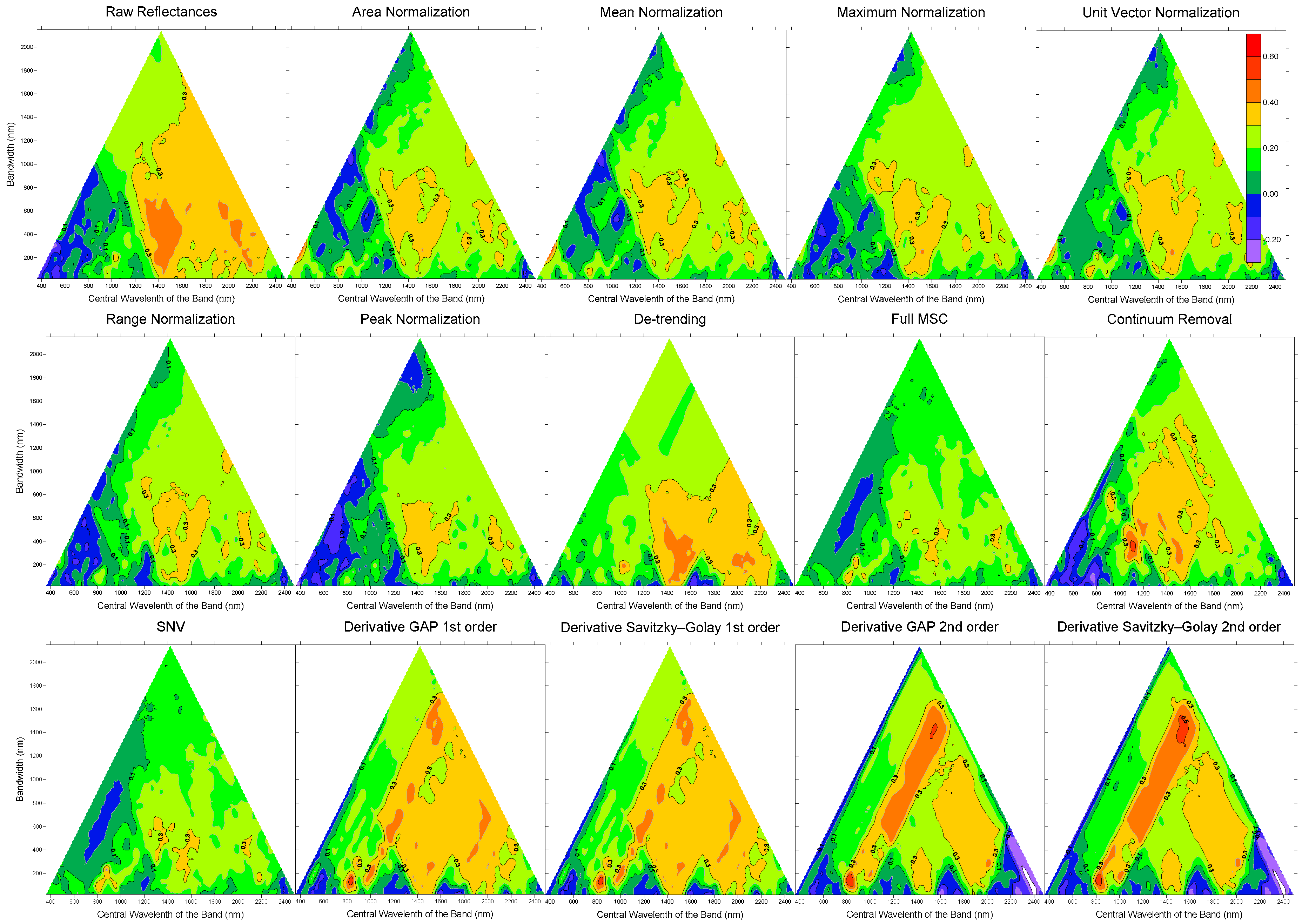
2.4.2. Transformation
2.5. Statistical Methods
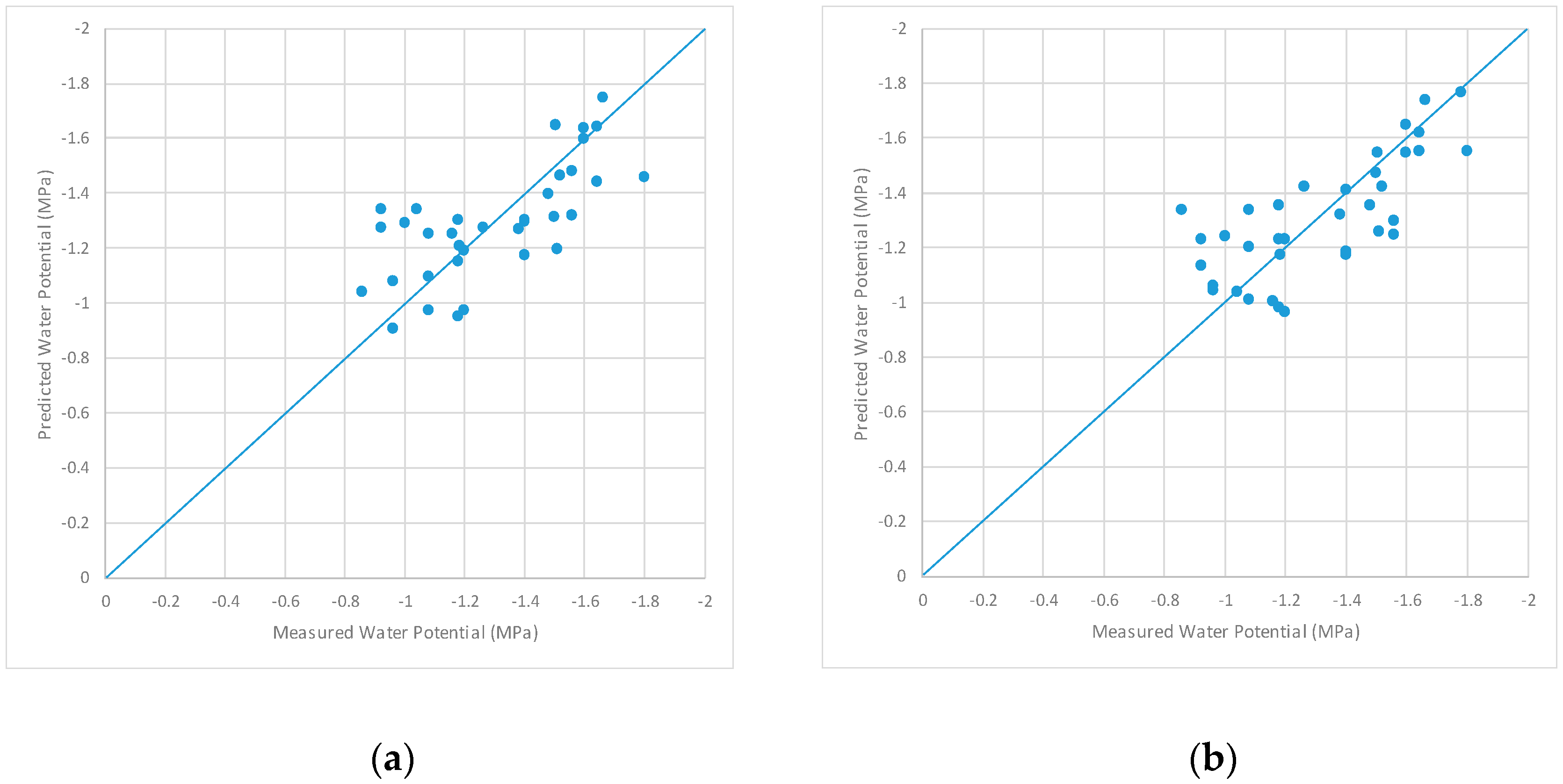
2.5.1. Partial Least Squares Regression
- (i)
- MWP versus full reflectance spectrum from 350 nm to 2500 nm with jump correction.
- (ii)
- MWP versus full reflectance spectrum from 350 nm to 2500 nm with jump correction and area normalization.
- (iii)
- MWP versus full reflectance spectrum from 350 nm to 2500 nm with jump correction and unit vector normalization.
- (iv)
- MWP versus full reflectance spectrum from 350 nm to 2500 nm with jump correction and mean normalization.
- (v)
- MWP versus full reflectance spectrum from 350 nm to 2500 nm with jump correction and maximum normalization.
- (vi)
- MWP versus full reflectance spectrum from 350 nm to 2500 nm with jump correction and unit range normalization.
- (vii)
- MWP versus full reflectance spectrum from 350 nm to 2500 nm with jump correction and peak normalization.
- (viii)
- MWP versus full reflectance spectrum from 350 nm to 2500 nm with jump correction and Norris Gap first-order derivative.
- (ix)
- MWP versus full reflectance spectrum from 350 nm to 2500 nm with jump correction and Norris Gap second-order derivative.
- (x)
- MWP versus full reflectance spectrum from 350 nm to 2500 nm with jump correction and Savitzky–Golay first-order derivative.
- (xi)
- MWP versus full reflectance spectrum from 350 nm to 2500 nm with jump correction and Savitzky–Golay second-order derivative.
- (xii)
- MWP versus full reflectance spectrum from 350 nm to 2500 nm with jump correction and SNV.
- (xiii)
- MWP versus full reflectance spectrum from 350 nm to 2500 nm with jump correction and MSC.
- (xiv)
- MWP versus full reflectance spectrum from 350 nm to 2500 nm with jump correction and de-trending.
- (xv)
- MWP versus full reflectance spectrum from 350 nm to 2500 nm with jump correction and CR transformation.
2.5.2. Cross-Validation
3. Results
4. Discussion
5. Conclusions
Author Contributions
Funding
Acknowledgments
Conflicts of Interest
References
- Flexas, J.; Galmés, J.; Gallé, A.; Gulias, J.; Pou, A.; Ribas, M.; Tomàs, M.; Medrano, H. Improving water use efficiency in grapevines: Potential physiological targets for biotechnological improvement. Aust. J. Grape Wine Res. 2010, 16, 106–121. [Google Scholar] [CrossRef]
- Lisar, S.Y.S.; Motafakkerazad, R.; Hossain, M.M.; Rahman, I.M.M. Water stress in plants: Causes, effects and responses. In Water Stress; Ismail, M.M.R., Hiroshi, H., Eds.; Intech Open: Rijeka, Croatia, 2012; pp. 1–15. [Google Scholar]
- Kennedy, J.A.; Matthews, M.A.; Waterhouse, A.L. Effect of maturity and vine water status on grape skin and wine flavonoids. Am. Enol. Vitic. 2002, 53, 268–274. [Google Scholar]
- Scholander, P.F.; Hammel, H.J.; Bradstreet, A.; Hemmingsen, E.A. Sap pressure in vascular plants. Science 1965, 148, 339–346. [Google Scholar] [CrossRef] [PubMed]
- Santos, A.O.; Kaye, O. Grapevine leaf water potential based upon near infrared spectroscopy. Sci. Agric. 2009, 66, 287–292. [Google Scholar] [CrossRef] [Green Version]
- Triolo, R.; Roby, J.P.; Plaia, A.; Hilbert, G.; Buscemi, S.; Di Lorenzo, R.; van Leeuwen, C. Hierarchy of factors impacting grape berry mass: Separation of direct and indirect effects on major berry metabolites. Am. J. Enol. Vitic. 2018, 69, 103–112. [Google Scholar] [CrossRef]
- Oumar, Z.; Mutanga, O. Predicting plant water content in Eucalyptus grandis forest stands in KwaZulu-Natal, South Africa using field spectra resampled to the Sumbandila Satellite Sensor. Int. J. Appl. Earth Obs. Geoinf. 2010, 12, 158–164. [Google Scholar] [CrossRef]
- Serrano, L.; Gonzalez-Flor, C.; Gorchs, G. Assessing vineyard water status using the reflectance-based water index. Agric. Ecosyst. Environ. 2010, 139, 490–499. [Google Scholar] [CrossRef]
- Zheng, L.; Wang, Z.; Sun, H.; Zhang, M.; Li, M. Real-time evaluation of corn leaf water content based on the electrical property of leaf. Comput. Electron. Agric. 2015, 112, 102–109. [Google Scholar] [CrossRef]
- Fuentes, A.; Vázquez-Gutiérrez, J.L.; Pérez-Gago, M.B.; Vonasek, E.; Nitin, N.; Dian, M.B. Application of non-destructive impedance spectroscopy to determination of the effect of temperature on potato microstructure and texture. J. Food Eng. 2014, 133, 16–22. [Google Scholar] [CrossRef]
- Jamaludin, D.; Abd-Aziz, S.; Ahmad, D.; Jaafar, H.Z.E. Impedance analysis of Labisia pumila plant water status. Inf. Process. Agric. 2015, 2, 161–168. [Google Scholar] [CrossRef]
- Mizukami, Y.; Sawai, Y.; Yamaguchi, Y. Moisture Content Measurement of Tea Leaves by Electrical Impedance and Capacitance. Biosyst. Eng. 2006, 93, 293–299. [Google Scholar] [CrossRef]
- He, J.-X.; Wang, Z.-Y.; Shi, Y.-L.; Qin, Y.; Zhao, D.-J.; Huang, L. A Prototype Portable System for Bioelectrical Impedance Spectroscopy. Sens. Lett. 2011, 9, 1151–1156. [Google Scholar] [CrossRef]
- Muñoz-Huerta, R.F.; Ortiz-Melendez, A.; Guevara-Gonzalez, R.G.; Torres-Pacheco, I.; Herrera-Ruiz, G.; Contreras-Medina, L.M.; Prado-Olivarez, J.V.; Ocampo-Velázquez, R. An Analysis of Electrical Impedance Measurements Applied for Plant N Status Estimation in Lettuce (Lactuca sativa). Sensors 2014, 14, 11492–11503. [Google Scholar] [CrossRef]
- Zimmermann, U.; Rüger, S.; Shapira, O.; Westhoff, M.; Wegner, L.-H.; Reuss, R.; Geßner, P.; Zimmermann, G.; Israeli, Y.; Zhou, A.; et al. Effects of environmental parameters and irrigation on the turgor pressure of banana plants measured using the non-invasive, online monitoring leaf patch clamp pressure probe. Plant Biol. 2010, 12, 424–436. [Google Scholar] [CrossRef]
- Rueger, S.; Ehrenberger, W.; Zimmermann, U.; Ben-Gal, A.; Agam, N.; Kool, D. The leaf patch clamp pressure probe: A new tool for irrigation scheduling and deeper insight into olive drought stress physiology. Acta Hortic. 2011, 888, 223–230. [Google Scholar] [CrossRef]
- Sancho-Knapik, D.; Gismero, J.; Asensio, A.; Peguero-Pina, J.J.; Fernández, V.; Gómez Álvarez-Arenas, T.; Gil-Pelegrín, E. Microwave l-band (1730 MHz) accurately estimates the relative water content in poplar leaves. A comparison with a near infrared water index (R1300/R1450). Agric. For. Meteorol. 2011, 151, 827–832. [Google Scholar] [CrossRef]
- Sancho-Knapik, D.; Gómez Álvarez-Arenas, T.; Peguero-Pina, J.J.; Gil-Pelegrín, E. Air-coupled broadband ultrasonic spectroscopy as a new non-invasive and non-contact method for the determination of leaf water status. J. Exp. Bot. 2010, 61, 1385–1391. [Google Scholar] [CrossRef] [Green Version]
- Sancho-Knapik, D.; Peguero-Pina, J.J.; Medrano, H.; Fariñas, M.D.; Gómez Álvarez-Arenas, T.; Gil-Pelegrín, E. The reflectivity in the S-band and the broadband ultrasonic spectroscopy as new tools for the study of water relations in Vitis vinifera L. Physiol. Plant. 2013, 148, 512–521. [Google Scholar] [CrossRef]
- Moshou, D.; Pantazi, X.; Kateris, D.; Gravalos, I. Water stress detection based on optical multisensor fusion with a least squares support vector machine classifier. Biosyst. Eng. 2014, 117, 15–22. [Google Scholar] [CrossRef]
- Hall, A.; Lamb, D.W.; Holzapfel, B.P.; Louis, J.P. Within-season temporal variation in correlations between vineyard canopy and wine grape composition and yield. Precis. Agric. 2011, 12, 103–117. [Google Scholar] [CrossRef]
- Strever, A.E. Estimating water stress in Vitis vinifera L. using field spectrometry: A preliminary study incorporating multispectral vigour classification. In Information and technology for sustainable fruit and vegetable production. In Proceedings of the Conference FRUTIC, Montpellier, France, 12–16 September 2005. [Google Scholar]
- Atzberger, C.; Guérif, M.; Baret, F.; Werner, W. Comparative analysis of three chemometric techniques for the spectroradiometric assessment of canopy chlorophyll content in winter wheat. Comput. Electron. Agric. 2010, 73, 165–173. [Google Scholar] [CrossRef]
- Cho, M.A.; Skidmore, A.; Corsi, F.; Van Wieren, S.E.; Sobhan, I. Estimation of green grass/herb biomass from airborne hyperspectral imagery using spectral indices and partial least squares regression. Int. J. Appl. Earth Obs. Geoinf. 2007, 9, 414–424. [Google Scholar] [CrossRef]
- González-Fernández, A.B.; Rodríguez-Pérez, J.R.; Marabel, M.; Álvarez-Taboada, F. Spectroscopic estimation of leaf water content in commercial vineyards using continuum removal and partial least squares regression. Sci. Hortic. 2015, 188, 15–22. [Google Scholar] [CrossRef]
- Zhang, Q.; Li, Q.; Zhang, G. Rapid determination of leaf water content using VIS/NIR spectroscopy analysis with wavelength selection. J. Spectrosc. 2012, 27, 93–105. [Google Scholar] [CrossRef]
- Mirzaie, M.; Darvishzadeh, R.; Shakiba, A.; Matkan, A.A.; Atzberger, C.; Skidmore, A. Comparative analysis of different uni- and multi-variate methods for estimation of vegetation water content using hyper-spectral measurements. Int. J. Appl. Earth Obs. Geoinf. 2014, 26, 1–11. [Google Scholar] [CrossRef]
- Zhao, K.; Valle, D.; Popescu, S.; Zhang, X.; Mallick, B. Hyperspectral remote sensing of plant biochemistry using Bayesian model averaging with variable and band selection. Remote Sens. Environ. 2013, 132, 102–119. [Google Scholar] [CrossRef]
- ASD Inc. 2012 FieldSpect4 User Manual 600979. Available online: https://www.malvernpanalytical.com/en/learn/knowledge-center/user-manuals/fieldspec-4-user-guide (accessed on 9 May 2019).
- Barnes, R.J.; Dhanoa, M.S.; Susan, S.J. Standard normal variate transformation and de-trending of near-infrared diffuse reflectance spectra. Appl. Spectrosc. 1989, 43, 772–777. [Google Scholar] [CrossRef]
- Vasques, G.M.; Grunwald, S.; Sickman, J.O. Comparison of multivariate methods for inferential modeling of soil carbon using visible/near-infrared spectra. Geoderma 2008, 146, 14–25. [Google Scholar] [CrossRef]
- Silalahia, D.D.; Midib, H.; Arasanb, J.; Mustafab, M.S.; Calimana, J.P. Robust generalized multiplicative scatter correction algorithm on pre-processing of near infrared spectral data. Vib. Spectrosc. 2018, 97, 55–65. [Google Scholar] [CrossRef]
- Norris, K.H.; Williams, P.C. Optimization of mathematical treatments of raw near-infrared signal in the measurement of protein in hard red spring wheat. i. influence of particle size. Cereal Chem. 1984, 61, 158–165. [Google Scholar]
- CAMO Software AS. The Unscrambler® X v10.3. User Manual. Version 1.0. Available online: https://www.camo.com/files/TheUnscramblerXv10.3-UserManual.zip (accessed on 9 May 2019).
- Syvilay, D.; Wilkie-Chancellier, N.; Trichereau, B.; Texier, A.; Martínez, L.; Serfaty, S.; Detalle, V. Evaluation of the standard normal variate method for Laser-Induced Breakdown Spectroscopy data treatment applied to the discrimination of painting layers. Spectrochim. Acta B 2015, 114, 38–45. [Google Scholar] [CrossRef]
- Maleki, M.R.; Mouazen, A.M.; Ramon, H.; De Baerdemaeker, J. Multiplicative scatter correction during on-line measurement with near infrared spectroscopy. Biosyst. Eng. 2007, 96, 427–433. [Google Scholar] [CrossRef]
- Huang, Z.; Turner, B.J.; Dury, S.J.; Wallis, I.R.; Foley, W.J. Estimating foliar nitrogen concentration from HYMAP data using continuum removal analysis. Remote Sens. Environ. 2004, 93, 18–29. [Google Scholar] [CrossRef]
- Kokaly, R.F.; Asner, G.P.; Ollinger, S.V.; Martin, M.E.; Wessman, C.A. Characterizing canopy biochemistry from imaging spectroscopy and its application to ecosystem studies. Remote Sens. Environ. 2009, 113, S78–S91. [Google Scholar] [CrossRef]
- Rodríguez-Pérez, J.R.; Riaño, D.; Carlisle, E.; Ustin, S.; Smart, D.R. Evaluation of hyperspectral reflectance indexes to detect grapevine water status in vineyards. Am. J. Enol. Vitic. 2007, 58, 302–317. [Google Scholar]
- Turner, N.C. Measurement of plant water status by the pressure chamber technique. Irrig. Sci. 1988, 9, 289–308. [Google Scholar] [CrossRef]
- Lau, I.C.; Cudahy, T.J.; Heinson, G.; Mauger, A.J.; James, P.R. Practical applications of hyperspectral remote sensing in regolith research. In Advances in Regolith; Roach, I.C., Ed.; CRC LEME: Adelaide, Australia, 2003; pp. 249–253. [Google Scholar]
- Geladi, P.; Kowalski, B.R. Partial least-squares regression: A tutorial. Anal. Chim. Acta 1986, 185, 1–17. [Google Scholar] [CrossRef]
- McLachlan, G.J.; Do, K.A.; Ambroise, C. Analyzing Microarray Gene Expression Data, 1st ed.; Wiley: New York, NY, USA, 2004; pp. 61–97. [Google Scholar]
- Richter, K.; Atzberger, C.; Hank, T.B.; Mauser, W. Derivation of biophysical variables from Earth observation data: Validation and statistical measures. J. Appl. Remote Sens. 2012, 6, 1–23. [Google Scholar] [CrossRef]
- Kokaly, R.F.; Clark, R.N. Spectroscopic determination of leaf biochemistry using band-depth analysis of absorption features and stepwise multiple linear regression. Remote Sens. Environ. 1999, 67, 267–287. [Google Scholar] [CrossRef]
- González-Fernández, A.B.; Rodríguez-Pérez, J.R.; Marcelo, V.; Valenciano, J.B. Using field spectrometry and a plant probe accessory to determine leaf water content in commercial vineyards. Agric. Water Manag. 2015, 156, 43–50. [Google Scholar] [CrossRef]
- Rodríguez-Pérez, J.R.; Ordóñez, C.; González-Fernández, A.B.; Sanz-Ablanedo, E.; Valenciano, J.B.; Marcelo, V. Leaf water content estimation by functional linear regression of field spectroscopy data. Biosyst. Eng. 2018, 36–46. [Google Scholar] [CrossRef]
- Milton, E.J.; Schaepman, M.E.; Anderson, K.; Kneubühler, M.; Fox, N. Progressing field spectroscopy. Remote Sens. Environ. 2009, 113, S92–S109. [Google Scholar] [CrossRef]
- Wang, J.; Xu, R.; Yang, S. Estimation of plant water content by spectral absorption features centered at 1450 nm and 1940 nm regions. Environ. Monit. Assess. 2009, 157, 459–469. [Google Scholar] [CrossRef]
- Shenk, J.S.; Workman, J.; Westerhaus, M.O. Application of NIR spectroscopy to agricultural products. In Handbook of Near-Infrared Analysis (Practical Spectroscopy Series), 2nd ed.; Burns, D.A., Ciurczak, E.D., Eds.; Dekker: New York, NY, USA, 2001; pp. 419–474. [Google Scholar]


© 2019 by the authors. Licensee MDPI, Basel, Switzerland. This article is an open access article distributed under the terms and conditions of the Creative Commons Attribution (CC BY) license (http://creativecommons.org/licenses/by/4.0/).
Share and Cite
González-Fernández, A.B.; Sanz-Ablanedo, E.; Gabella, V.M.; García-Fernández, M.; Rodríguez-Pérez, J.R. Field Spectroscopy: A Non-Destructive Technique for Estimating Water Status in Vineyards. Agronomy 2019, 9, 427. https://0-doi-org.brum.beds.ac.uk/10.3390/agronomy9080427
González-Fernández AB, Sanz-Ablanedo E, Gabella VM, García-Fernández M, Rodríguez-Pérez JR. Field Spectroscopy: A Non-Destructive Technique for Estimating Water Status in Vineyards. Agronomy. 2019; 9(8):427. https://0-doi-org.brum.beds.ac.uk/10.3390/agronomy9080427
Chicago/Turabian StyleGonzález-Fernández, Ana Belén, Enoc Sanz-Ablanedo, Víctor Marcelo Gabella, Marta García-Fernández, and José Ramón Rodríguez-Pérez. 2019. "Field Spectroscopy: A Non-Destructive Technique for Estimating Water Status in Vineyards" Agronomy 9, no. 8: 427. https://0-doi-org.brum.beds.ac.uk/10.3390/agronomy9080427