Appendix A. Supporting Information
In order to account for effectiveness of IGS analysis in bacterial species here we report the data for two other species:
B. subtilis and
P. haloplanktis. In fact, from
Figure A1,
Figure A2,
Figure A3,
Figure A4,
Figure A5,
Figure A6,
Figure A7,
Figure A8,
Figure A9,
Figure A10 and
Figure A11 and
Table A1 and
Table A2 have been obtained for the former species, while from
Figure A12,
Figure A13,
Figure A14,
Figure A15,
Figure A16,
Figure A17,
Figure A18,
Figure A19,
Figure A20,
Figure A21 and
Figure A22 and
Table A3 and
Table A4 refer to the latter one. Both sets of pictures and tables follow the same ordering adopted for
E. coli in the main text.
First of all, we can remark that the global BCA is quite similar for the three species, although the cluster BCA exhibits peculiar features, typical of each species. This notwithstanding, the figures appearing in the table of the three bacterial species (
Table 1 and
Table 2 for
E. coli,
Table A1 and
Table A2 for
B. subtilis,
Table A3 and
Table A4 for
P. haloplanktis) are quite similar to each other in all of the three species, thus testifying an overall robustness of the structural features in the gene networks associated to clusters.
The remarkable difference is highlighted in
Figure A17: the crescent like shape of point distribution in the clustering space is due to the presence of a relative small subset of IGSs, that contain an unusually high amount of G and C nucleotides. AS a final remark it is worth pointing out that, while the conclusion drawn about the COG functional enrichment analysis provides quite similar results for
E. coli and
B. subtilis, one of the three clusters of
P. haloplanktis lacks any indication of functional enrichment.
Anyway, despite the appearance of different features, we can say that the general conclusions drawn by the IGS analysis for E. coli apply to the two other species.
Figure A1.
B. subtilis. The frequency of IGRs versus their length, , expressed in bps. The binning is over 100 bps. The distribution is truncated at 12,000 bps.
Figure A1.
B. subtilis. The frequency of IGRs versus their length, , expressed in bps. The binning is over 100 bps. The distribution is truncated at 12,000 bps.
Figure A2.
B. subtilis. The frequency of RIGRs versus their length, , expressed in bps. The binning is over 5 bps and the distribution is truncated at 600 bps. The peak close to 0 is due to the simplifying assumption of setting to 0 the contribution from overlapping coding regions.
Figure A2.
B. subtilis. The frequency of RIGRs versus their length, , expressed in bps. The binning is over 5 bps and the distribution is truncated at 600 bps. The peak close to 0 is due to the simplifying assumption of setting to 0 the contribution from overlapping coding regions.
Figure A3.
B. subtilis. The frequency of the different SDSs located upstream the TSC, listed along the horizontal axis.
Figure A3.
B. subtilis. The frequency of the different SDSs located upstream the TSC, listed along the horizontal axis.
Figure A4.
B. subtilis. The frequency of the position of the SDSs upstream the TSC.
Figure A4.
B. subtilis. The frequency of the position of the SDSs upstream the TSC.
Figure A5.
B. subtilis. The first twenty eigenvalues in ascending order of the normalized Laplacian matrix obtained by the alignment of the IGSs. Red crosses and blue circles correspond to different values of the similarity threshold, determined by the two statistical approaches described in
Section 2.3.2. A better discrimination of the three main eigenvalues is obtained for a higher similarity threshold (blue crosses), which corresponds to the second statistical approach, better suited for short sequences, as the annotated IGSs.
Figure A6.
B. subtilis. Distribution of points in the clustering space relative to the alignment of the IGSs. Each point represents an IGS and the color code corresponds to the three clusters identified by the
Clustering Algorithm described in
Section 2.3.3.
Figure A6.
B. subtilis. Distribution of points in the clustering space relative to the alignment of the IGSs. Each point represents an IGS and the color code corresponds to the three clusters identified by the
Clustering Algorithm described in
Section 2.3.3.
Figure A7.
B. subtilis. Distribution of silhouette values relative to the clustering of the IGSs. On the vertical axis we report the frequency of IGSs versus the silhouette value s; this value is between −1 and +1. The average values are 0.42 for all the clusters.
Figure A7.
B. subtilis. Distribution of silhouette values relative to the clustering of the IGSs. On the vertical axis we report the frequency of IGSs versus the silhouette value s; this value is between −1 and +1. The average values are 0.42 for all the clusters.
Figure A8.
B. subtilis. BCA of the IGSs: on the vertical axis we report the density
(see
Section 2.4) of each of the four nucleotides
A (blue), T (red), G (yellow), C (purple) as a function of the position
ℓ along the annotated 2338 IGSs.
Figure A8.
B. subtilis. BCA of the IGSs: on the vertical axis we report the density
(see
Section 2.4) of each of the four nucleotides
A (blue), T (red), G (yellow), C (purple) as a function of the position
ℓ along the annotated 2338 IGSs.
Table A1.
Coexpression networks in B. subtilis. We compare the features of the coexpression networks for each cluster between the three clusters obtained by the clustering method and other three clusters obtained by averaging over a 1000 random samplings of the IGSs of B. subtilis.
Table A1.
Coexpression networks in B. subtilis. We compare the features of the coexpression networks for each cluster between the three clusters obtained by the clustering method and other three clusters obtained by averaging over a 1000 random samplings of the IGSs of B. subtilis.
| | | | | | | | | | | |
|---|
| C0 | 749 | 1341 | 25 | 25.7 | 14.4 | −0.05 | 63 | 169.6 | 189.7 | −0.56 |
| C1 | 856 | 1346 | 41 | 30.6 | 15.6 | 0.67 | 417 | 199.1 | 201.2 | 1.08 |
| C2 | 884 | 1487 | 16 | 32.3 | 16.5 | −0.99 | 28 | 217.5 | 212.2 | −0.89 |
Figure A9.
B. subtilis. Base composition analysis in the clusters of the IGSs: on the vertical axis we report the density
(see
Section 2.4) of each of the four nucleotides
A (blue), T (red), G (yellow), C (purple) as a function of the position
ℓ along the IGS belonging to the clusters C0 (left panel), C1 (central panel) and C2 (right panel).
Figure A10.
B. subtilis. Smoothed Base composition analysis in the clusters of the IGSs: on the vertical axis we report the averaged density
for
bps (see
Section 2.4) of each of the four nucleotides A (blue), T(red), G (yellow), C (purple) as a function of the position
ℓ along the IGSs belonging to the clusters C0 (left panel), C1 (central panel) and C2 (right panel).
Table A2.
Cooccurrence networks in B. subtilis. We compare the features of the cooccurrence networks for each cluster between the three clusters obtained by the clustering method and other three clusters obtained by averaging over a 1000 random samplings of the IGSs of B. subtilis.
Table A2.
Cooccurrence networks in B. subtilis. We compare the features of the cooccurrence networks for each cluster between the three clusters obtained by the clustering method and other three clusters obtained by averaging over a 1000 random samplings of the IGSs of B. subtilis.
| | | | | | | | | | | |
|---|
| C0 | 749 | 1341 | 73 | 50.2 | 16.6 | 1.38 | 162 | 119.8 | 60.9 | −0.69 |
| C1 | 856 | 1346 | 71 | 63.1 | 17.4 | 0.45 | 198 | 158.3 | 77.0 | 0.52 |
| C2 | 884 | 1487 | 38 | 67.4 | 18.4 | −1.60 | 85 | 170.1 | 84.2 | −1.01 |
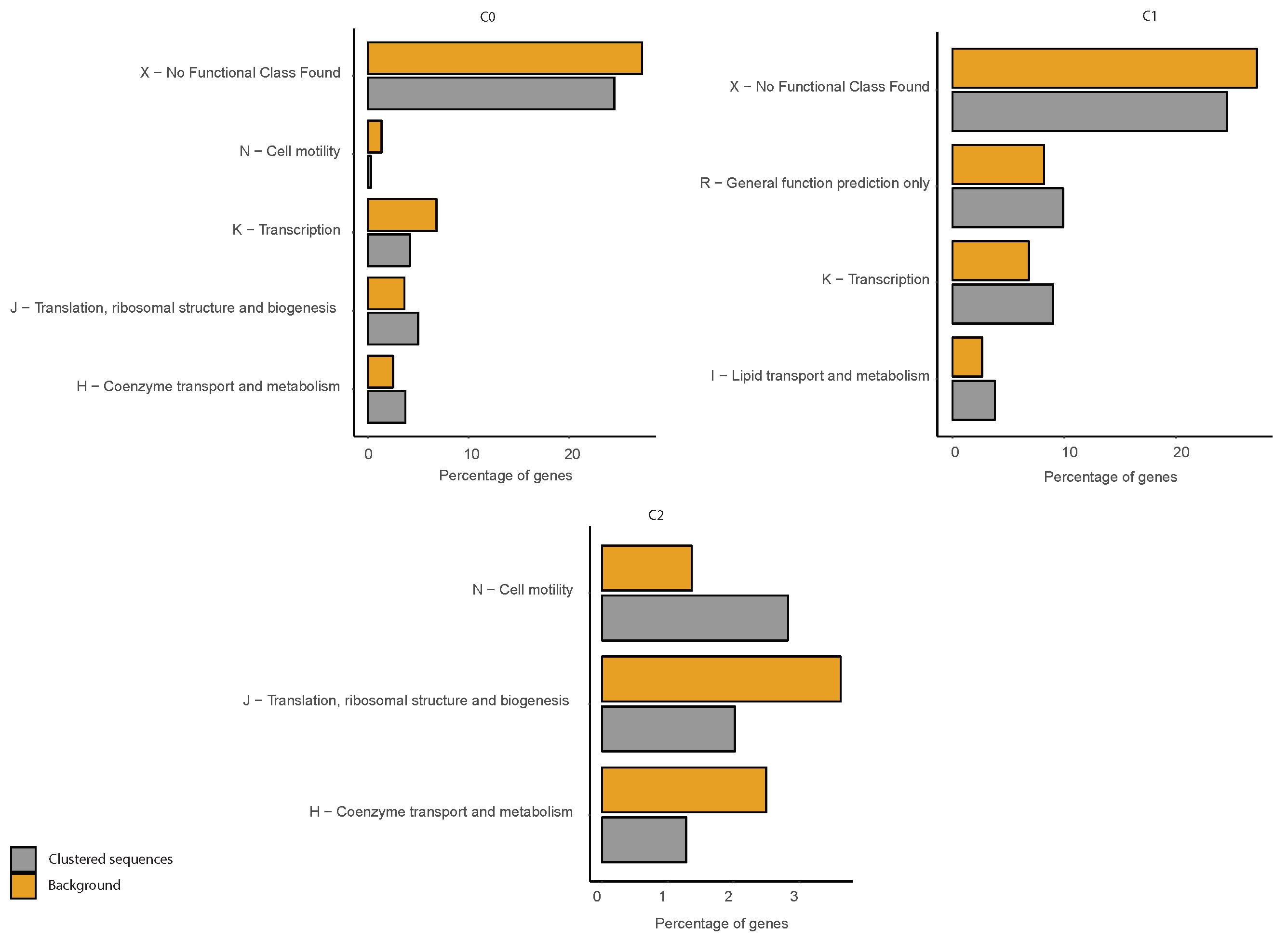
Figure A11.
COG functional enrichment analysis of clustered genes in B. subtilis. We report the significantly enriched or depleted COG functional categories belonging to each of the identified clusters (C0, C1, C2) in respect to the genome background. Clustered Sequences refers to the functional annotation of the sequences that were clustered according to our method (i.e., after the analysis of IGSs) in each of the three clusters. Genome background refers to the functional annotation of the entire genome (i.e., of each gene of the organism considered).
Figure A12.
P. haloplanktis. The frequency of IGRs versus their length, , expressed in bps. The binning is over 100 bps. The distribution is truncated at 12,000 bps.
Figure A12.
P. haloplanktis. The frequency of IGRs versus their length, , expressed in bps. The binning is over 100 bps. The distribution is truncated at 12,000 bps.
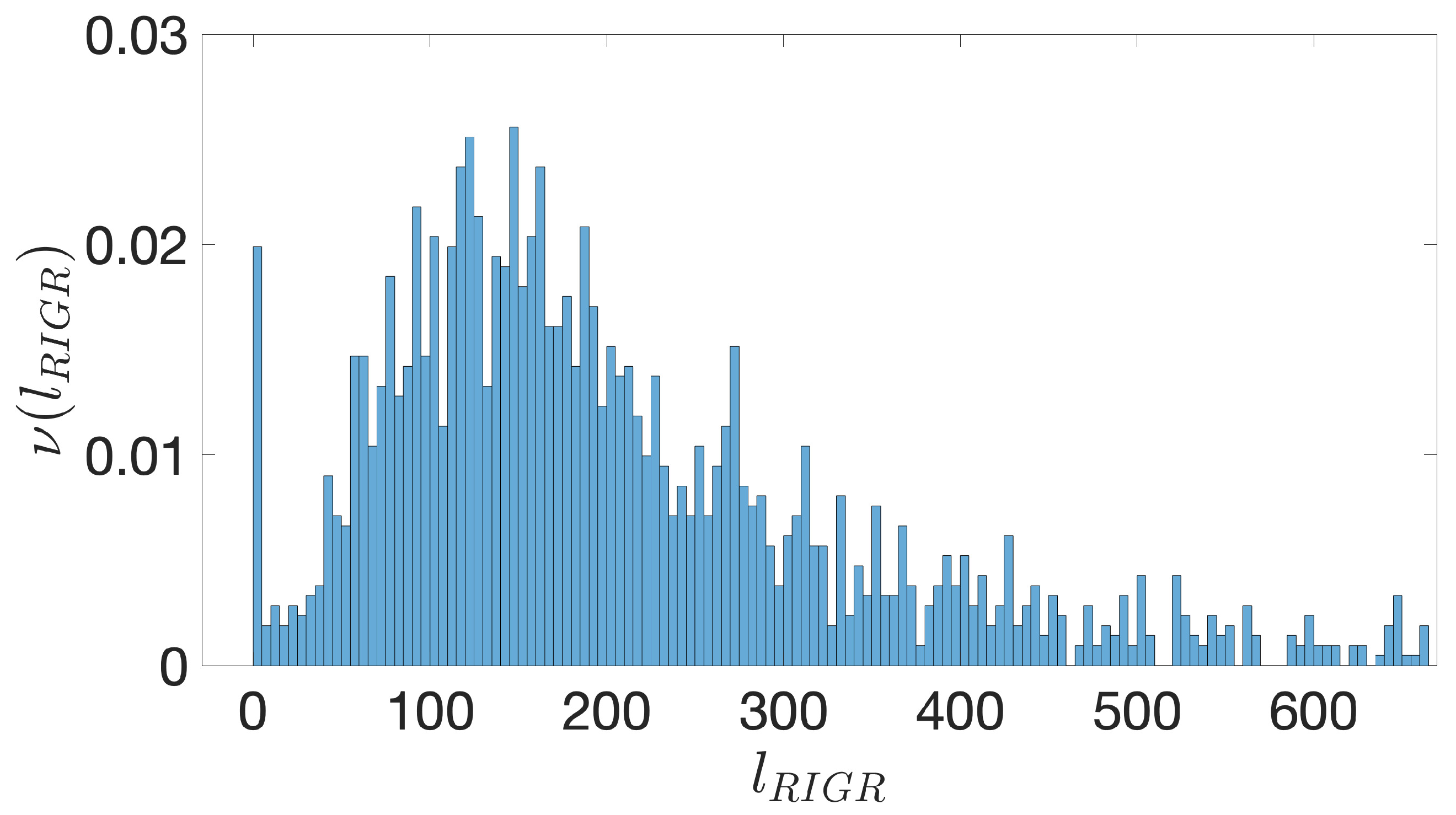
Figure A13.
P. haloplanktis. The frequency of RIGRs versus their length, , expressed in bps. The binning is over 5 bps and the distribution is truncated at 600 bps. The peak close to 0 is due to the simplifying assumption of setting to 0 the contribution from overlapping coding regions.
Figure A13.
P. haloplanktis. The frequency of RIGRs versus their length, , expressed in bps. The binning is over 5 bps and the distribution is truncated at 600 bps. The peak close to 0 is due to the simplifying assumption of setting to 0 the contribution from overlapping coding regions.
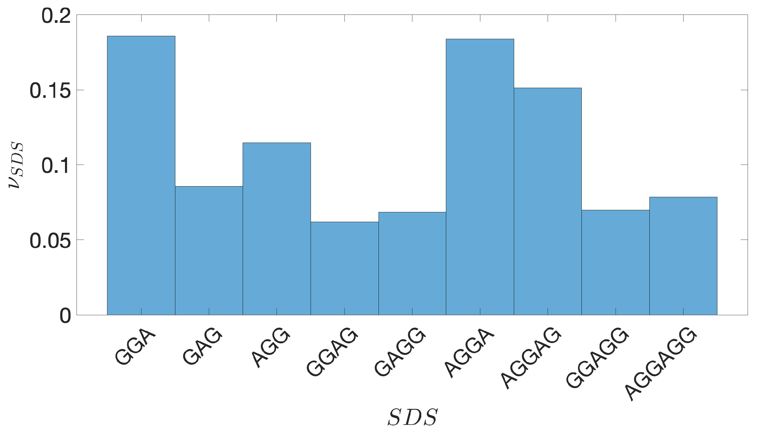
Figure A14.
P. haloplanktis. The frequency of the different SDSs located upstream the TSC, listed along the horizontal axis.
Figure A14.
P. haloplanktis. The frequency of the different SDSs located upstream the TSC, listed along the horizontal axis.
Figure A15.
P. haloplanktis. The frequency of the position of the SDSs upstream the TSC.
Figure A15.
P. haloplanktis. The frequency of the position of the SDSs upstream the TSC.
Figure A16.
P. haloplanktis. The first twenty eigenvalues in ascending order of the normalized Laplacian matrix obtained by the alignment of the IGSs. Red crosses and blue circles correspond to different values of the similarity threshold, determined by the two statistical approaches described in
Section 2.3.2. A better discrimination of the three main eigenvalues is obtained for a higher similarity threshold (blue crosses), which corresponds to the second statistical approach, better suited for short sequences, as the annotated IGSs.
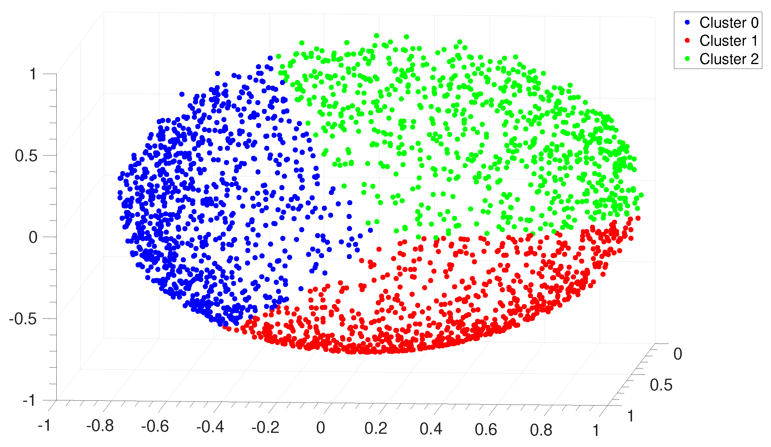
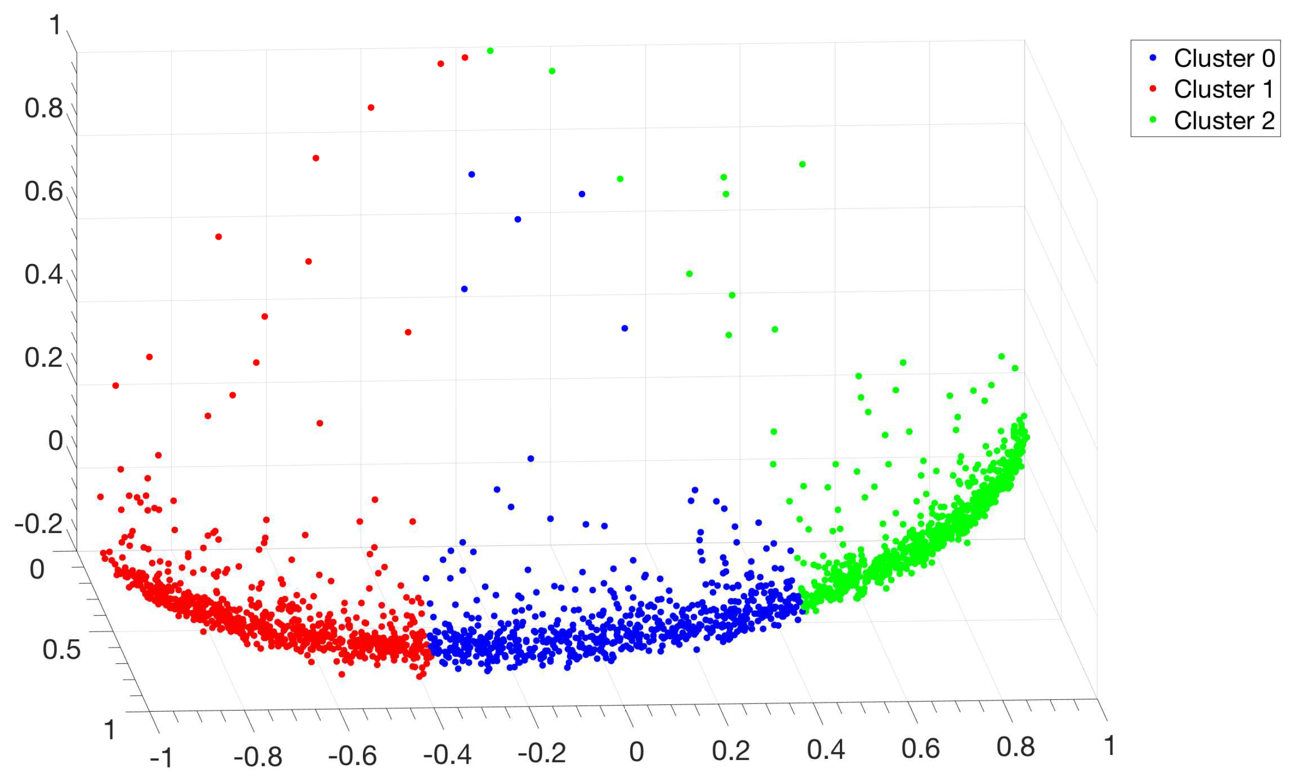
Figure A17.
P. haloplanktis. Distribution of points in the clustering space relative to the alignment of the IGSs. Each point represents an IGS and the color code corresponds to the three clusters identified by the
Clustering Algorithm described in
Section 2.3.3. This seemingly unusual distribution of points in the clustering space is due to the presence of scattered points which correspond to IGSs very far from the centroid of the different clusters. This is peculiar of this bacterium; on the other hand if these few atypical IGSs would be eliminated from the sample one should recover a point distribution very similar to those reported in
Figure 8 and
Figure A6.
Figure A18.
P. haloplanktis. Distribution of silhouette values relative to the clustering of the IGSs. On the vertical axis we report the frequency of IGSs versus the silhouette value s; this value is between −1 and +1. The average values are 0.48 for cluster C0, 0.56 for C1 and 0.58 for C2.
Figure A18.
P. haloplanktis. Distribution of silhouette values relative to the clustering of the IGSs. On the vertical axis we report the frequency of IGSs versus the silhouette value s; this value is between −1 and +1. The average values are 0.48 for cluster C0, 0.56 for C1 and 0.58 for C2.
Figure A19.
P. haloplanktis. BCA of the IGSs: on the vertical axis we report the density
(see
Section 2.4) of each of the four nucleotides
A (blue), T(red), G (yellow), C (purple) as a function of the position
ℓ along the annotated 2091 IGSs.
Figure A19.
P. haloplanktis. BCA of the IGSs: on the vertical axis we report the density
(see
Section 2.4) of each of the four nucleotides
A (blue), T(red), G (yellow), C (purple) as a function of the position
ℓ along the annotated 2091 IGSs.
Table A3.
Coexpression networks in P. haloplanktis. We compare the features of the coexpression networks for each cluster between the three clusters obtained by the clustering method and other three clusters obtained by averaging over a 1000 random samplings of the IGSs of P. haloplanktis.
Table A3.
Coexpression networks in P. haloplanktis. We compare the features of the coexpression networks for each cluster between the three clusters obtained by the clustering method and other three clusters obtained by averaging over a 1000 random samplings of the IGSs of P. haloplanktis.
| | | | | | | | | | | |
|---|
| C0 | 664 | 1074 | 22 | 23.0 | 12.0 | −0.08 | 36 | 102.7 | 108.8 | −0.61 |
| C1 | 718 | 1182 | 47 | 26.8 | 13.8 | 1.46 | 305 | 124.6 | 128.4 | 1.40 |
| C2 | 709 | 1079 | 24 | 26.1 | 12.0 | −0.16 | 42 | 122.1 | 121.6 | −0.66 |
Figure A20.
P. haloplanktis. Base composition analysis in the clusters of the IGSs: on the vertical axis we report the density
(see
Section 2.4) of each of the four nucleotides
A (blue), T(red), G (yellow), C (purple) as a function of the position
ℓ along the IGS belonging to the clusters C0 (left panel), C1 (central panel) and C2 (right panel).
Figure A21.
P. haloplanktis. Smoothed Base composition analysis in the clusters of the IGSs: on the vertical axis we report the averaged density
for
bps (see
Section 2.4) of each of the four nucleotides A (blue), T(red), G (yellow), C (purple) as a function of the position
ℓ along the IGSs belonging to the clusters C0 (left panel), C1 (central panel) and C2 (right panel).
Table A4.
Cooccurrence networks in P. haloplanktis. We compare the features of the cooccurrence networks for each cluster between the three clusters obtained by the clustering method and other three clusters obtained by averaging over a 1000 random samplings of the IGSs of P. haloplanktis.
Table A4.
Cooccurrence networks in P. haloplanktis. We compare the features of the cooccurrence networks for each cluster between the three clusters obtained by the clustering method and other three clusters obtained by averaging over a 1000 random samplings of the IGSs of P. haloplanktis.
| | | | | | | | | | | |
|---|
| C0 | 664 | 1074 | 58 | 45.3 | 21.2 | 0.60 | 129 | 104.8 | 71.7 | 0.34 |
| C1 | 718 | 1182 | 89 | 51.4 | 21.5 | 1.75 | 441 | 120.3 | 77.1 | 4.16 |
| C2 | 709 | 1079 | 36 | 51.8 | 22.5 | −0.70 | 76 | 122.6 | 86.2 | −0.54 |
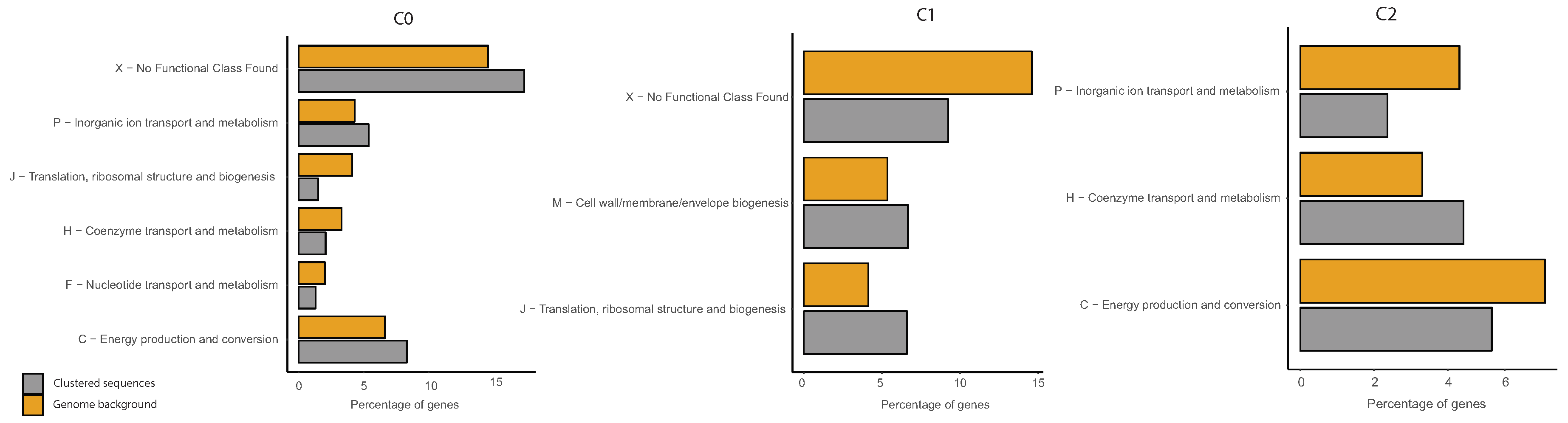
Figure A22.
COG functional enrichment analysis of clustered genes in P. haloplanktis. We report the significantly enriched or depleted COG functional categories belonging to each of the identified clusters (C0, C1, C2) in respect to the genome background. Clustered Sequences refers to the functional annotation of the sequences that were clustered according to our method (i.e., after the analysis of IGSs) in each of the three clusters. Genome background refers to the functional annotation of the entire genome (i.e., of each gene of the organism considered).

 ,
, 


