Study on Scale-Selective Initial Perturbation for Regional Ensemble Forecast

1
Nanjing University of Information Science & Technology, Nanjing 210044, China
2
Institute of Urban Meteorology, China Meteorological Administration, Beijing 100089, China
3
Numerical Weather Prediction Centre, China Meteorological Administration, Beijing 100081, China
*
Author to whom correspondence should be addressed.
Atmosphere 2019, 10(5), 285; https://0-doi-org.brum.beds.ac.uk/10.3390/atmos10050285
Submission received: 25 April 2019
/
Revised: 16 May 2019
/
Accepted: 16 May 2019
/
Published: 21 May 2019
(This article belongs to the Special Issue Advancements in Mesoscale Weather Analysis and Prediction)
Abstract
:To improve the skills of the regional ensemble forecast system (REFS), a modified ensemble transform Kalman filter (ETKF) initial perturbation strategy was developed. First, sensitivity tests were conducted to investigate the influence of the perturbation scale on the ensemble spread growth and forecast skill. In addition, the scale characteristic of the forecast error was analyzed based on the results of these tests, and a new initial condition perturbation method was developed through scale-selection of the ETKF perturbations, namely, ETKF-SS (scale-selective ETKF). The performances of the ETKF-SS scheme and the original ETKF (hereinafter referred to as ETKF) scheme were tested and compared. The results showed that the large-scale perturbations were much easier to grow than the original ETKF perturbations. In addition, scale analysis of the forecast error showed that the large-scale errors showed significant growth at the upper levels, while the small and meso-scale errors grew fast at the lower levels. The comparison results of the ETKF-SS and the ETKF showed that the ETKF-SS perturbations had more obvious growth than the ETKF perturbations, and the ETKF-SS perturbations in the short-term forecast lead times were more precise than the ETKF perturbations. The ensemble forecast verification results showed that the ETKF-SS ensemble had a larger spread and smaller root mean square error than the ETKF at short forecast lead times, while the probabilistic scores of the ETKF-SS also outperformed those of the ETKF method. In addition, the ETKF-SS ensemble can provide a better precipitation forecast than the ETKF.
1. Introduction
The non-linear and unstable characteristics of the atmosphere lead to intrinsic uncertainty in numerical weather prediction (NWP), which means slight errors in the initial state will amplify quickly and affect forecast skills [1]; in addition, the imperfections of the numerical model may cause forecast error. To solve the problem of forecast uncertainty caused by the initial state error, model error, and chaos of the atmosphere, ensemble forecast technology was proposed by Leith et al. [2], and it has become an effective tool in many NWP centers.
In recent years, it is particularly important and urgent to improve the quality of high-impact weather prediction (such as tropical cyclones and heavy rainfall). Hazardous high-impact weather is related mostly to small-scale dynamical mechanisms, which contain more forecast uncertainties. Therefore, more investigations are needed to deepen understanding of the uncertainty source related to high-impact weather to improve forecast skills. The regional ensemble forecast system (REFS) is an effective tool for local high-impact weather forecasting, and it has become a hot topic in present research [3,4,5].
Since initial uncertainty can dramatically affect the forecast quality, the initial condition (IC) perturbation method is crucial for the REFS. One popular way to generate IC perturbations is dynamical downscaling [6,7,8,9], as it is easy to implement and can produce promising ensemble spread, but the drawback of dynamical downscaling perturbations is the lack of small-scale components. Some others introduce traditional methods to the REFS originally applied in the Global Ensemble Forecast System, such as breeding growing mode (BGM), singular vectors (SVs), and ensemble transform Kalman filter (ETKF) [10,11,12,13], and there are some methods specifically designed for REFS [14]. It is proved that these methods can produce sufficient small- or meso-scale perturbations consistent with the resolution of the regional model; however, these perturbations lack large-scale uncertainty information. Therefore, when applied to REFS, these traditional methods face the problem of creating enough large-scale information important to the REFS.
The REFS has been running operationally for several years by the China Meteorological Administration (CMA). The system was constructed based on the meso-scale model of GRAPES-REFS (Global and Regional Assimilation and Prediction Enhanced System-Regional Ensemble Forecast System), which was developed by the CMA. The GRAPES-REFS uses ETKF to generate IC perturbations. Similar to the BGM, the ETKF method produces perturbations by forecast cycle in the regional model, and therefore, these perturbations are able to contain sufficient small-scale uncertainty information. However, some problems arise in the operational run, one of which is that the system exhibits underspread characteristics. A previous study proved that the ETKF (as well as some other cycling methods) can generate many small-scale perturbations when applied to the REFS; however, these small-scale perturbations are not as easy to grow as large-scale perturbations. Toth and Kalnay [15] noted that many small-scale perturbations will lose energy during the model integration. These small-scale perturbations can be viewed as “noise” and the ensemble spread will be restricted if the IC perturbations contain too much noise; thereafter, how to remove these useless perturbation components while conserving useful perturbations has become a notable issue.
To improve the performance of GRAPES-REFS, this paper conducted a modification on the IC perturbation strategy, that is, partly removing the unnecessary small-scale components within the ETKF perturbations and conserving some sufficient large-scale components. The aim of this modification was to improve the spread of REFS by removing the useless perturbations while keeping the useful perturbations untouched.
The rest of the paper is organized as follows: in Section 2, the GRAPES-REFS system and methodology is discussed; Section 3 covers the sensitivity tests to investigate the influence of the perturbation scale on the ensemble spread growth, and the scale characteristic of the model forecast error is analyzed to provide a reference for the scale-selective method, meanwhile the scale-selective method on IC perturbations is also discussed in Section 3; a summary of these results along with a discussion is provided in Section 4.
2. Methodology
2.1. System Description
This study is based on the regional ensemble forecast system of GRAPES-REFS, which consists of a meso-scale model named GRAPES-MESO (Version 4.0). The domain of this regional model covers the whole area of China with a horizontal resolution of 15 km. GRAPES-REFS includes one control forecast and 14 perturbed members and is run twice (initiated at 00 UTC and 12 UTC) each day with a forecast lead time of 72 h.
2.2. Perturbation Method and Filter Scheme
The scale-selective scheme was based on the ETKF method and a digital filter process, both of which are described in this section.
Similar to the traditional IC perturbation method of BGM and ensemble transform (ET) [16], ETKF [17] is based on the theory of breeding that the fastest growing component of the perturbations will be obtained through breeding cycles, and additionally, the ETKF method can adopt observational information when generating perturbations and the perturbation structure of each member is orthogonal. In this study, the IC perturbations were generated by the ETKF method, which is based on the hypothesis that the forecast covariance matrices and analysis covariance matrices can be represented by forecast perturbations and analysis perturbations . The relationship between and is established after solving the optimal data assimilation equation. As a result, the forecast perturbation can be transformed to the analysis perturbation through transformation matrix :
where forecast perturbations are listed as columns in matrix , analysis perturbations are listed as columns in matrix , and is the transformation matrix. The measure of inflating the analysis perturbation’s amplitude is conducted to ensure the ensemble forecast variance is consistent with the control forecast error variance. In addition to centering the perturbed members around the control forecasts, an inflation factor and a simple spherical centering scheme is introduced.
where is the inflation factor and [18] is the matrix that centers the perturbed members around the control forecast.
The scale-selective process will act directly on the ETKF analysis perturbation state once the perturbation states are formed in each ETKF cycle (see Figure 1).
For each member i, a low-pass filter will be used on the perturbation state , which is generated by the ETKF, and the final IC perturbation will be obtained after this filtering progress; thus, the function is as follows:
In this study, a two-dimensional discrete cosine transform low-pass filter (2D-DCT) [19] was applied. This low-pass filter is suitable for separating horizontal meteorological fields into different scales. Figure 2 shows an example function of the low-pass filter, which is also commonly called the amplitude response function of the filter. For this low-pass filter, all scales shorter than “w1” km were removed and all scales larger than “w2” km were preserved. For the scales between “w1” and “w2”, the physical field was partly removed through a gradually varying transfer function with a soft cut-off [20,21]. Additionally, the 2D-DCT is also used as a scale-analyzing tool since it can transform the two-dimensional state into a power spectrum.
2.3. Experimental Data
The T639 (model spectral triangular truncation was T639 with 60 vertical levels, corresponding to a 30-km horizontal resolution) global ensemble forecast data provided background states and lateral boundary conditions (LBCs) for the GRAPES-REFS, and the analysis states of the GRAPES-REFS control corresponding to each forecast lead time were used as the true state to verify the variables at different pressure levels, while the precipitation was verified against observed cumulative precipitation from 2507 meteorological stations in China.
3. Results
3.1. The Impact of IC Perturbation Scale on Perturbation Growth
To investigate whether the “scale” is an important factor affecting the perturbation growth, some sensitivity tests were conducted in this section by selecting a particularly large-scale part out of the original ETKF perturbation. The perturbation scale-selections were conducted by the aforementioned 2D-DCT low-pass filter. In this section, two filter strategies were implemented, one was 480–960 km (all scales smaller than 480 km were removed, while scales larger than 960 km were preserved, hereinafter named ETKF-filter1), and the other was 960–1920 km (hereinafter named ETKF-filter2). These two schemes were compared with the original ETKF in terms of perturbation growth (see Table 1). All three experiments were conducted in the same REFS environment for a period of 10 days.
Figure 3 shows the horizontal distribution of zonal wind perturbation at the 850 hPa level for ETKF, ETKF-filter1, and ETKF-filter2. It can be seen that the ETKF perturbation (Figure 3a) contains sufficient small-scale information, but the structure is not clear enough. Because the two kinds of filtering schemes extracted some larger perturbations from the original ETKF perturbation state, for example, ETKF-filter1 completely removed the components smaller than 480 km, the spatial distribution of ETKF-filter1 exhibits more obvious meso- and large-scale structural features (Figure 3b). Furthermore, the ETKF-filter2 perturbation state retains a much larger perturbation scale than that of ETKF and ETKF-filter2, which basically only keeps the synoptic scale perturbations.
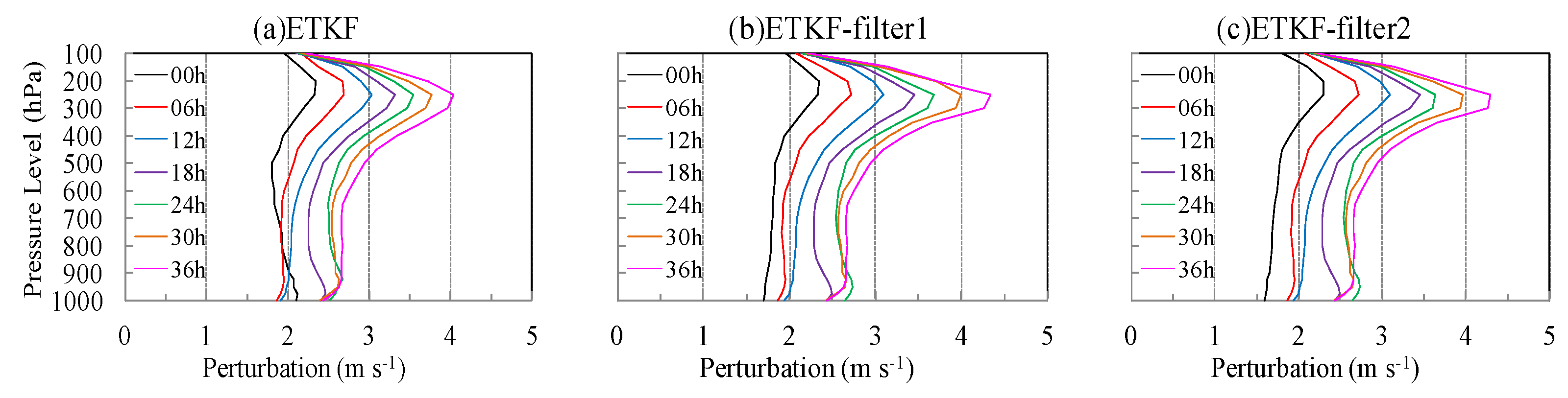
Figure 4 shows the 10-day averaged absolute value profile of zonal wind perturbation at different forecast times. We can see that the ETKF perturbation (Figure 4a) can reach a peak value of 2.3 m s−1 (approximately 200–300 hPa) or more at the initial time, but the growth is relatively slow, and the peak value can reach 4.0 m s−1 at a forecast lead time of 36 h. For ETKF-filter1 (Figure 4b), although the initial perturbation magnitude was smaller than ETKF due to the filtering process, the growth was fast enough that the peak value could reach 4.3 m s−1 for a 36-h forecast lead time. The perturbation magnitude of ETKF-filter2 (Figure 4c) can also increase to 4.26 m s−1 for the 36 h forecast. When comparing lower levels, we found that ETKF-filter1 and ETKF-filter2 had less amplitude than the ETKF at the initial time, but the perturbation growth was very obvious, and the amplitude of both ETKF-filter1 and ETKF-filter2 perturbations was equal to that of ETKF or slightly larger for the long-range forecast.
The above analysis indicates that the large-scale perturbations were prone to grow, and the reason for this phenomenon was that large-scale perturbations have more organized structures and can, thus, develop much easier with dynamic flow in the model. The results in this section can provide a practical way to solve the problem of under-spread, which exists commonly in the REFS.
3.2. The Characteristics of the Error Scale
As the resolution of the model increases, its effect on simulating small-scale weather phenomena gradually improves. It is known that these convective-scale and storm-scale weather phenomena mainly develop at the middle and lower levels of the model’s atmosphere, so the uncertainty of such weather should be addressed by small-scale perturbations at these levels. The above results show that large-scale perturbations have a good ability to develop, so it is worthwhile to study whether we can remove small-scale perturbations at the upper level and only retain large-scale perturbations. At the same time, we need to keep the perturbations at the lower levels unchanged since the small-scale perturbations are critical at these levels. In this section, the scale features of the forecast error will be analyzed using a single model. It will make us fully understand the error characteristics at different levels in terms of scale, because forecast errors are closely related to forecast uncertainty, and this work can provide a reference for the scale-selection of IC perturbations.
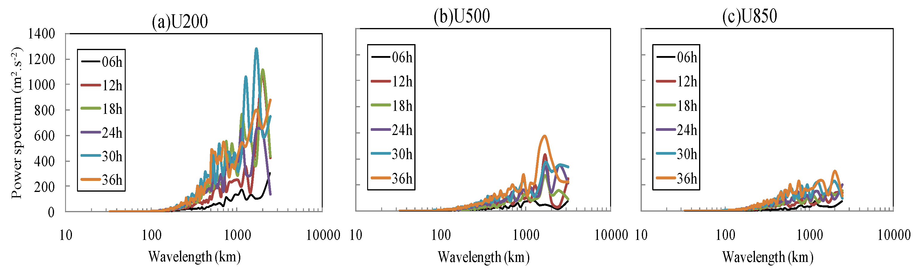
The 2D-DCT method was used as a scale analysis tool and can convert the forecast error field into a power spectrum field. Figure 5 shows the forecast error power spectrum as a function of wavelength for different forecast lead times. It can be seen that for zonal wind at 200 hPa (Figure 5a), the most powerful component of the forecast error was mainly concentrated on the scale of 200 km or more, and the large-scale spectra magnitude was obviously larger than that of the small-scale spectra magnitude. Figure 5b shows that the most powerful scale was above 1000 km for zonal wind at 500 hPa, and the large-scale spectra magnitude was larger than the small-scale spectra magnitude. In regard to 850 hPa (Figure 5c), although the large-scale power spectrum amplitude was larger, the magnitude difference between the large-scale and small-scale spectra was not as remarkable as that of the upper levels. These results indicate that the large-scale forecast error plays a dominant role at the high level, while in the middle and lower levels, the small-scale error was relatively significant. Similar results can be found for other variables (not shown).
The above results make us believe that the large-scale forecast error occupies an important proportion at a high level in the model. Therefore, the forecast uncertainty at the high level mainly comes from large-scale flow, while small-scale errors account for a very important part at the low level.
3.3. Initial Perturbation Construction Based on Scale-Selection
3.3.1. Scale-Selection of the ETKF Perturbation
It can be seen from the above analysis that large-scale perturbations have good growing ability, and for the higher level, especially above the troposphere, small-scale perturbations have difficulty developing. Therefore, it is necessary to filter out small-scale perturbations at the high level and to retain large-scale perturbations as much as possible.
Based on the above hypothesis, this section carried out related comparative tests. Two ensemble experiments were designed for comparison. One was the ETKF control scheme with the IC perturbation generated by the original ETKF, and the other was the scale-selective ETKF scheme (hereinafter referred to as ETKF-SS), which introduces a filter process into the ETKF scheme. The system settings of the two schemes were the same except for the IC perturbation scheme.
According to the scale characteristics of the forecast error given in Section 3.2, the filtering settings were different for various variables at different levels, so the terms “small” and “large” are reflective of the relative relationship between the two components that need to be filtered out and need to be preserved, and the criterion varies with different levels; that is, for the upper levels, more small-scale components will be filtered out to ensure only the large-scale (mostly the synoptic scale that is characterized by baroclinic instability) perturbations dominate, while for the lower levels, only part of the small-scale (mostly the scales with dissipating gravity waves) components will be filtered out because some of the small-scale perturbations need to be conserved. Considering that the variable of the specific humidity only exists at low levels with reasonable small-scale characteristics, no filter process will be applied to it. The details of the settings can be referenced in Table 2. The consecutive experiments are conducted within a period from 29 July 2015 to 15 August 2015 to investigate the performance of the ETKF-SS and ETKF schemes.
3.3.2. The Evolution Characteristics of the Perturbation
First, the evolution characteristics of the perturbations are compared in this section. Figure 6 shows the horizontal distribution of zonal wind perturbation at 500 hPa and synoptic flow of the control analysis with forecast lead times of 00, 12, and 24 h, and both ensembles were initiated at 12 UTC on 29 July 2015. It can be seen that the ETKF perturbation at the initial time (Figure 6a) had a larger amplitude and more small-scale components, while ETKF-SS (Figure 6d) had a smaller perturbation magnitude at a larger scale than that of ETKF. For the forecast lead time of 12 h, the ETKF perturbation showed some limited growth at some areas such as the West Pacific; however, the ETKF-SS perturbation exhibited obvious growth in that area. For the forecast lead time of 24 h, the perturbation patterns for both schemes were much more similar, with the ETKF-SS perturbation magnitude being slightly larger.
Figure 7 shows the vertical profile of the zonal wind perturbation with a time series of 00–36 h. Compared to that of ETKF (Figure 7a), the initial (00 h) perturbation amplitude of ETKF-SS (Figure 7b) was relatively small, but the perturbation growth for ETKF-SS was more remarkable. The largest perturbation amplitude for ETKF-SS at 36 h was approximately 4.3 m s−1, while that for ETKF was 4.0 m s−1. This result indicates that the scale-selection can help the perturbation develop.
3.3.3. The Correlation of Perturbation and Forecast Error
A larger spread is desirable for REFS since it always exhibits underspread characteristics; however, it is also crucial that the ensemble spread can precisely represent the growing characteristic of the forecast error, which can make the system reliable. Studies by Toth et al. [22] and Zhu et al. [23] suggest that a good ensemble forecast system can capture the forecast uncertainty under different weather conditions, which means the ensemble perturbation pattern corresponds well to the forecast error distribution within model space, and we call such ability of the ensemble perturbation “the precision of the ensemble”.
Here, we introduce tests for the ensemble perturbation precision. Consider a scatter plot in which the ordinate and abscissa of each point are given by the forecast error and ensemble perturbation, respectively, on a two-dimensional grid space. The forecast error used here is given by the absolute value of the control forecast:
where is the control forecast and is the corresponding analysis. The ensemble perturbation is:
where is the forecast of the kth member, is the ensemble mean, and N is the ensemble size.
Figure 8 presents the scatter plot of the 15-day averaged ensemble perturbation and forecast error for a 500 hPa temperature, with forecast lead times of 18 h and 24 h. It can be seen from the 18 h forecast of ETKF (Figure 8a) that the ensemble perturbations underestimate the forecast error for a large amount of grid points, since many sample points are located under the diagonal line; however, the perturbation magnitude of ETKF-SS can also be smaller than that of the forecast error, but more sample points are close to the diagonal line. For the 24 h forecast, the results were similar to those of the 18 h forecast; the ETKF (Figure 8c) perturbations underestimated the forecast error, whereas the ETKF-SS (Figure 8d) perturbations gave a better result. This result indicates that the perturbations of ETKF-SS were better than those of ETKF at representing the magnitude and location of the forecast error.
3.3.4. Verification of the Ensemble Forecast
One of the criteria for measuring the quality of an ensemble forecast system is whether the ensemble spread is roughly equivalent to the root mean square error (rmse). Figure 9a–c shows the one-month averaged ensemble mean RMSE and ensemble spread of three variables of the zonal wind at 200 hPa (U200), temperature at 500 hPa (T500), and zonal wind at 850 hPa (U850), respectively. It turns out that for all of these variables, the ETKF-SS showed smaller RMSE and larger spread at all forecast aging times, and similar results can also be observed for other variables at different levels (not shown). These results suggest that the ETKF-SS ensemble can truly enhance the accuracy of the ensemble mean forecast.
To further study the improvement effect of the ETKF-SS on regional ensemble prediction, the continuous grade probability score (CRPS) was calculated for the ETKF and ETKF-SS. The CRPS is a commonly used ensemble prediction probability score [24], which can quantitatively compare the difference between the predicted cumulative distribution probability and the observed cumulative distribution probability. The CRPS score is negatively oriented, where higher values indicate poorer probabilistic performance of the ensemble forecast system. Figure 9d–f shows the time-series of the CRPS scores for the ETKF and ETKF-SS. It is clear that the ETKF-SS performed better (with a smaller CRPS value) than the ETKF for all the variables at all forecast lead times. Specifically, the ETKF-SS outperformed the ETKF at short forecast lead times for upper-level variables, and the ETKF-SS had obviously better performance for U200 within the 24 h forecast, while for the lower level, the advantage occurred throughout the 72 h forecast. The CRPS verification on other variables can give similar results (not shown).
Outlier was another commonly used probability score, which refers to the frequency at which observations fall outside the members of the ensemble. A more reliable ensemble prediction has a smaller outlier value. As seen from Figure 9e–i, the ETKF-SS had a smaller outlier value than the ETKF for all the variables, indicating that the observations were more likely to fall within the ETKF-SS forecast.
It can be seen from the above results that the ETKF-SS had obvious advantages compared to the ETKF in the short forecast lead times, indicating that the scale-selective method can improve the quality of the ensemble perturbation and furthermore improve the ensemble probability score.
3.3.5. A Precipitation Case Study
To evaluate the performance of the ETKF and ETKF-SS on precipitation forecast, a typical heavy precipitation case in the summer of 2015 was studied. The forecast started at 12 UTC on 29 July 2015.
Figure 10a shows the 24-h cumulative precipitation of the observation from 00 UTC 30 July 2015 to 00 UTC 31 July 2015. It can be seen that the range of precipitation was so wide that it affected most parts of North China; the strong precipitation center was located in central and southern Shandong, and the precipitation level reached more than 100 mm.
Figure 10b–g shows the 24-h cumulative precipitation forecast in the form of ensemble mean, maximum value, and probability over 25 mm for the ETKF and ETKF-SS, respectively. It can be found that the ETKF ensemble mean precipitation forecast (Figure 10b) deviated from the observation, and it did not give a good simulation on the strong precipitation center located in Shangdong, indicating that most of the members did not predict the precipitation center well. Figure 10c shows the ensemble mean forecast of ETKF-SS; we can see that the position of the precipitation over 25 mm was much closer to the observation. The maximum precipitation forecast of the ETKF (Figure 10d) presents a large magnitude in the northern part of Shandong, but it was significantly northward from the observation, while the maximum precipitation forecast of the ETKF-SS (Figure 10e) shows that the precipitation over 25 mm and 50 mm covered the central and southern parts of Shandong, which corresponds well to the observation. From the probability forecast over 25 mm, we found that the ETKF (Figure 10f) had a large probability mainly in the north of Shandong, and the indicative signals given in other areas were relatively small. In contrast, the ETKF-SS ensemble forecast (Figure 10g) presents a probability over 40% in central Shandong, which is more consistent with the observation.
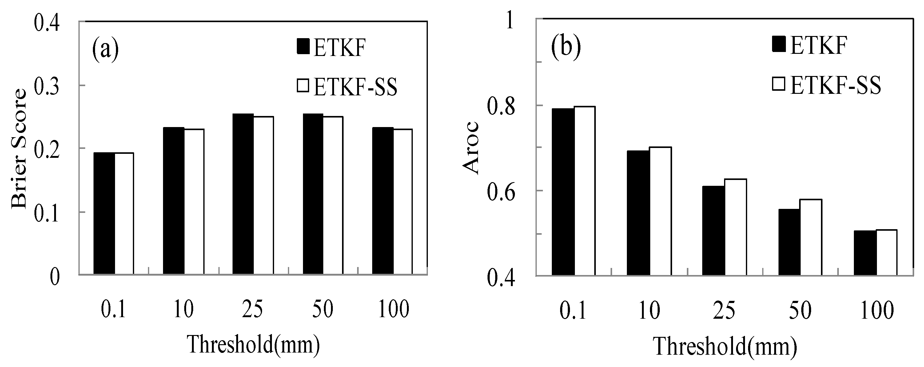
The performances of the two ensembles with respect to their precipitation forecasts were examined by computing the one-month statistical Brier score (BS) and area of relative operating characteristic (AROC), which are appropriate for measuring the probability forecast skill of an ensemble in terms of the quantitative precipitation forecast. The BS measures the mean squared difference between the predicted probability and the observed occurrence of an event, producing a value between zero and one, with a smaller value indicating better performance. The AROC denotes the relative relationship between the hit rate and the false alarm rate for a threshold of an event, where a higher AROC means a higher hit rate and better probability forecast, and vice versa [25]. Figure 11 shows the Brier score and AROC of 24-h cumulative precipitation on 31 July 2015. As shown in Figure 11a, the Brier score of the ETKF-SS performed slightly worse in light and medium precipitation but better than the ETKF in heavy precipitation over 25 mm; the AROC of the ETKF-SS was also better than that of the ETKF (Figure 11b), especially in heavy precipitation. In general, the ETKF-SS scheme can improve the probability precipitation skills, especially for the heavy precipitation forecast.
This improvement of the heavy precipitation forecast is reasonable because for a numerical simulation, it is the interaction of multiple-scale systems that can trigger precipitation in the model, such as the synoptic-scale forcing, strong ascent, and vapor transport. Since the spatial distribution of heavy precipitation is greatly affected by the atmospheric flow, if we want to acquire a better precipitation location, the perturbations should be more precise to represent uncertainties related to all scales, including the uncertainties of the synoptic flow. For GRAPES-REFS, the probability forecast from the ETKF-SS can not only maintain small-scale information at low levels, but also modify large-scale synoptic forcing information at the upper levels, and this modification on upper-level large-scale flow can help to improve the synoptic circulation factors, thereby improving the spatial distribution of heavy precipitation.
4. Summary and Discussion
To improve the initial perturbation quality and the forecast skill of the regional ensemble forecast, the scale-selective ETKF scheme is developed in this study. Multiple tests have been carried out to strengthen the basis of this new method, with the evaluation of this method presented in many aspects. The conclusions are as follows:
First, in order to understand the influence of perturbation scale on the GRAPES-REFS, filter sensitivity tests with three schemes were carried out, namely, the original ETKF perturbation, an ETKF perturbation at a larger scale, and an ETKF perturbation at the largest scale. Continuous tests were carried out with these three schemes, and the results show that the growth of the original ETKF perturbation was relatively slow, while the growth of perturbations at the larger and largest scales were more rapid.
The growing characteristic of the single-model forecast error was analyzed with respect to different levels and different variables, and the results indicated that the small-scale error growth was limited at the high level, and the forecast uncertainty at high levels was dominated by large-scale error.
The scale-selective ETKF scheme was designed and evaluated. This method partly removes small-scale perturbation components at the upper and middle levels with only large-scale components conserved, while most small-scale perturbation components were maintained at the lower level. The continuous experiments on both the original ETKF scheme and scale-selective ETKF scheme were conducted, and the results showed that the perturbation growth of the scale-selective ETKF scheme was obviously faster than that of the original ETKF, indicating that large-scale perturbations play a good role in promoting the spread growth. The result of the correlation between perturbation and forecast error shows that the perturbation quality of scale-selective ETKF is better than that of ETKF, which can better identify the forecast error’s magnitude at different locations. The verification results showed that the scale-selective ETKF scheme can effectively improve the quality of REFS, giving that it can increase the ensemble spread and decrease the RMSE. Other probabilistic forecast scores indicate that the scale-selective ETKF scheme has superior performance at short forecast lead times. The result of the precipitation case study showed that the scale-selective ETKF can significantly improve the probability forecast of heavy rain.
In addition to the good performance at solving the “underspread” problem and improving the precipitation forecast, this scale-selective method also has some aspects that need further investigation. First is the filter scale setting; in this study, the filter scales were selected according to the characteristics of forecast error scale at different levels; however, some experiments need to be conducted to verify whether the filter scale is perfect or not. Second, it should be noted that filtering may affect the dynamical coordination within the model space. In this study, since the filtering object was only the “perturbation” and not all the model variables, the dynamical coordination problem between model variables did not emerge; in addition, the filtering did not change the distribution pattern of the perturbation within the model space, and the dynamical coordination is not destroyed at present, but this is indeed a factor that needs attention in future trials. Finally, since the model perturbations and lateral boundary condition perturbations for both ETKF and ETKF-SS systems were the same, the different performances of the two systems due to the different IC perturbations schemes were limited, and more efforts need to be directed to the model perturbations and lateral boundary condition perturbations to further improve the REFS.
Author Contributions
H.Z. conceived and designed the experiments. The paper was written by Y.X. with significant contributions from J.C.
Funding
This study was supported by the National Natural Science Foundation of China (Grant No. 41605082).
Conflicts of Interest
The authors declare no conflicts of interest.
References
- Lorenz, E.N. Deterministic nonperiodic flow. J. Atmos. Sci. 1963, 20, 130–141. [Google Scholar] [CrossRef]
- Leith, C.E. Theoretical skill of Monte Carlo forecasts. Mon. Weather Rev. 1974, 102, 409–418. [Google Scholar] [CrossRef]
- Sindic-Rancic, G.; Toth, Z.; Kalnay, E. Storm scale ensemble experiments with ARPS model: Preliminary results. In Proceedings of the 12th Conference on Numerical Weather Prediction, Phoenix, AZ, USA, 11–16 January 1998; pp. 279–280. [Google Scholar]
- Stensrud, D.J.; Yussouf, N. Reliable probabilistic quantitative precipitation forecasts from a short-range ensemble forecasting system. Weather Forecast. 2007, 22, 3–17. [Google Scholar] [CrossRef]
- Zhang, H.; Chen, J.; Zhi, X.; Li, Y.L.; Sun, Y. Study on the application of GRAPES regional ensemble prediction system. Meteorol. Mon. 2014, 40, 1076–1087. (In Chinese) [Google Scholar]
- Marsigli, C.; Boccanera, F.; Montani, A.; Paccagnella, T. The COSMO-LEPS mesoscale ensemble system: Validation of the methodology and verification. Nonlinear Process. Geophys. 2005, 12, 527–536. [Google Scholar] [CrossRef]
- Frogner, I.L.; Haakenstad, H.; Iversen, T. Limited-area ensemble predictions at the Norwegian Meteorological Institute. Q. J. R. Meteorol. Soc. 2008, 132, 2785–2808. [Google Scholar] [CrossRef]
- Bowler, N.E.; Arribas, A.; Mylne, K.R.; Robertson, K.B.; Beare, S.E. The MOGREPS short-range ensemble prediction system. Q. J. R. Meteorol. Soc. 2008, 134, 703–722. [Google Scholar] [CrossRef]
- Ji, Y.; Chen, J.; Jiao, M. The preliminary experiment of GRAPES-MESO ensemble prediction based on TIGGE data. Meteorol. Mon. 2011, 37, 392–402. (In Chinese) [Google Scholar]
- Stensrud, D.J.; Brooks, H.E.; Du, J.; Tracton, M.S.; Rogers, E. Using ensembles for short-range forecasting. Mon. Weather Rev. 1999, 127, 433–446. [Google Scholar] [CrossRef]
- Du, J.; DiMego, G.; Tracton, M.S.; Zhou, B. NCEP short-range ensemble forecasting (SREF) system: Multi-IC, multi-model and multi-physics approach. Res. Act. Atmos. Ocean. Model. 2003, 33, 5–9. [Google Scholar]
- Long, K.; Chen, J.; Ma, X.; Ji, Y. The preliminary study on ensemble prediction of GRAPES-MESO based on ETKF. J. Chengdu Univ. Inf. Technol. 2011, 26, 37–46. (In Chinese) [Google Scholar]
- Zhang, H.; Chen, J.; Zhi, X.; Wang, Y. A Comparison of ETKF and Downscaling in a Regional Ensemble Prediction System. Atmosphere 2015, 6, 341–360. [Google Scholar] [CrossRef]
- Chen, J.; Xue, J.; Yan, H. A new initial perturbation method of ensemble mesoscale heavy rain prediction. J. Atmos. Sci. 2005, 29, 717–726. (In Chinese) [Google Scholar]
- Toth, Z.; Kalnay, E. Ensemble forecasting at NCEP and the breeding method. Mon. Weather Rev. 1997, 125, 3297–3319. [Google Scholar] [CrossRef]
- Wei, M.; Toth, Z.; Wobus, R.; Zhu, Y. Initial Perturbations Based on the Ensemble Transform (ET) Technique in the NCEP Global Operational Forecast system. Tellus 2008, 60A, 62–79. [Google Scholar] [CrossRef]
- Wang, X.; Bishop, C.H. A comparison of breeding and ensemble transform Kalman filter ensemble forecast schemes. J. Atmos. Sci. 2003, 60, 1140–1158. [Google Scholar] [CrossRef]
- Wang, X.; Bishop, C.H.; Julier, S.J. Which Is Better, an Ensemble of Positive–Negative Pairs or a Centered Spherical Simplex Ensemble? Mon. Weather Rev. 2004, 132, 1590–1605. [Google Scholar] [CrossRef]
- Denis, B.; Coôteé, J.; Laprise, R. Spectral decomposition of two-dimensional atmospheric fields on limited-area domains using discrete cosine transform (DCT). Mon. Weather Rev. 2002, 130, 1812–1829. [Google Scholar] [CrossRef]
- Wang, Y.; Bellus, M.; Geleyn, J.F.; Ma, X.; Tian, W.; Weidle, F. A New Method for Generating Initial Condition Perturbations in a Regional Ensemble Prediction System: Blending. Mon. Weather Rev. 2014, 142, 2043–2059. [Google Scholar] [CrossRef] [Green Version]
- Zhang, H.; Chen, J.; Zhi, X.; Wang, Y.; Wang, Y. Study on Multi-Scale Blending Initial Condition Perturbations for a Regional Ensemble Prediction System. Adv. Atmos. Sci. 2015, 32, 1143–1155. [Google Scholar] [CrossRef]
- Toth, Z.; Zhu, Y.; Marchok, T. The use of ensembles to identify forecasts with small and large uncertainty. Weather Forecast. 2001, 16, 436–477. [Google Scholar] [CrossRef]
- Zhu, Y.; Toth, Z.; Wobus, R.; Richardson, D.; Mylne, K. The economic value of ensemble-based weather forecasts. Bull. Am. Meteorol. Soc. 2002, 83, 73–83. [Google Scholar] [CrossRef]
- Hersbach, H. Decomposition of the continuous ranked probability score for ensemble prediction systems. Weather Forecast. 2000, 15, 559–570. [Google Scholar] [CrossRef]
- Duan, J.; Wang, P.; Wu, H. The ensemble forecasting verification on the summer Eurasian middle-high latitude circulation. J. Appl. Meteorol. Sci. 2009, 20, 56–61. (In Chinese) [Google Scholar]
Figure 1.
Process of the regional ensemble forecast system utilizing a filter process for the ensemble transform Kalman filter (ETKF) update cycle.
Figure 1.
Process of the regional ensemble forecast system utilizing a filter process for the ensemble transform Kalman filter (ETKF) update cycle.

Figure 2.
An example function of the 2D-DCT filter method.

Figure 3.
The horizontal distribution of the perturbation of the zonal wind: (a) ETKF, (b) ETKF-filter1, and (c) ETKF-filter2.
Figure 3.
The horizontal distribution of the perturbation of the zonal wind: (a) ETKF, (b) ETKF-filter1, and (c) ETKF-filter2.

Figure 4.
Ten-day averaged absolute value profile of zonal wind perturbation at different forecast times: (a) ETKF, (b) ETKF-filter1, and (c) ETKF-filter2.
Figure 4.
Ten-day averaged absolute value profile of zonal wind perturbation at different forecast times: (a) ETKF, (b) ETKF-filter1, and (c) ETKF-filter2.

Figure 5.
Forecast error power spectra as a function of wavelength at different forecast lead times: (a) U200, (b) U500, and (c) U850.
Figure 5.
Forecast error power spectra as a function of wavelength at different forecast lead times: (a) U200, (b) U500, and (c) U850.

Figure 6.
Horizontal distribution of zonal wind perturbation (shaded) and geopotential height (line) of the control analysis at 500 hPa; ETKF: (a) 00 h, (b) 06 h, (c) 12 h; ETKF-SS: (d) 00 h, (e) 06 h, (f) 12 h.
Figure 6.
Horizontal distribution of zonal wind perturbation (shaded) and geopotential height (line) of the control analysis at 500 hPa; ETKF: (a) 00 h, (b) 06 h, (c) 12 h; ETKF-SS: (d) 00 h, (e) 06 h, (f) 12 h.

Figure 7.
Vertical profile of the zonal wind perturbation at different forecast lead times of 00–36 h. (a) ETKF and (b) ETKF-SS.
Figure 7.
Vertical profile of the zonal wind perturbation at different forecast lead times of 00–36 h. (a) ETKF and (b) ETKF-SS.

Figure 8.
Scatter plot of the relationship between ensemble perturbation and forecast error for a 500 hPa temperature. (a) 18 h forecast for ETKF, (b) 18 h forecast for ETKF-SS, (c) 24 h forecast for ETKF, (d) 24 h forecast for ETKF-SS.
Figure 8.
Scatter plot of the relationship between ensemble perturbation and forecast error for a 500 hPa temperature. (a) 18 h forecast for ETKF, (b) 18 h forecast for ETKF-SS, (c) 24 h forecast for ETKF, (d) 24 h forecast for ETKF-SS.

Figure 9.
The verification of ensemble forecast of ETKF and ETKF-SS, (a–c), the time-series of rmse and spread of U200 hPa, T850 hPa, and U850 hPa, respectively; (d–f), the time-series of CRPS of U200 hPa, T850 hPa, and U850 hPa, respectively; (g–i), the time-series of outlier of U200 hPa, T850 hPa, and U850 hPa, respectively.


Figure 10.
The verification of precipitation. (a) 24-h cumulative precipitation of the observation from 00 UTC 30 July 2015 to 00 UTC 31 July 2015; (b,c), 24-h cumulative precipitation ensemble average forecast of the ETKF and ETKF-SS; (d,e), the maximum precipitation forecast of the ETKF and ETKF-SS; (f,g), the probability prediction of precipitation greater than 25 mm for the ETKF and ETKF-SS.


Figure 11.
The score of the 24-h cumulative precipitation on 31 July 2015; (a) Brier score and (b) AROC.
Figure 11.
The score of the 24-h cumulative precipitation on 31 July 2015; (a) Brier score and (b) AROC.


Table 1.
Configuration of the filter settings for the three tests.
| Test Scheme | Filtering Scale (km) |
|---|---|
| ETKF | none |
| ETKF-filter1 | 480–960 |
| ETKF-filter2 | 960–1920 |
Table 2.
The scale-selection scheme of the filtering of various variables in different levels (w1–w2).
Table 2.
The scale-selection scheme of the filtering of various variables in different levels (w1–w2).
| Level (hPa) | Zonal Wind (u) | Meridional Wind (v) | Potential Temperature (θ) | Exner Pressure (π) |
|---|---|---|---|---|
| 150 | 960–1920 km | 960–1920 km | 1920–3840 km | 1920–3840 km |
| 200 | 960–1920 km | 960–1920 km | 1920–3840 km | 1920–3840 km |
| 300 | 480–960 km | 480–960 km | 1920–3840 km | 1920–3840 km |
| 400 | 480–960 km | 480–960 km | 960–1920 km | 1920–3840 km |
| 500 | 480–960 km | 480–960 km | 960–1920 km | 960–1920 km |
| 600 | 480–960 km | 480–960 km | 960–1920 km | 960–1920 km |
| 700 | 240–480 km | 240–480 km | 480–960 km | 960–1920 km |
| 800 | 120–240 km | 120–240 km | 240–480 km | 480–960 km |
| 850 | 60–120 km | 60–120 km | 240–480 km | 480–960 km |
| 925 | 60–120 km | 60–120 km | 240–480 km | 480–960 km |
© 2019 by the authors. Licensee MDPI, Basel, Switzerland. This article is an open access article distributed under the terms and conditions of the Creative Commons Attribution (CC BY) license (http://creativecommons.org/licenses/by/4.0/).
Share and Cite
MDPI and ACS Style
Xia, Y.; Zhang, H.; Chen, J. Study on Scale-Selective Initial Perturbation for Regional Ensemble Forecast. Atmosphere 2019, 10, 285. https://0-doi-org.brum.beds.ac.uk/10.3390/atmos10050285
AMA Style
Xia Y, Zhang H, Chen J. Study on Scale-Selective Initial Perturbation for Regional Ensemble Forecast. Atmosphere. 2019; 10(5):285. https://0-doi-org.brum.beds.ac.uk/10.3390/atmos10050285
Chicago/Turabian StyleXia, Yu, Hanbin Zhang, and Jing Chen. 2019. "Study on Scale-Selective Initial Perturbation for Regional Ensemble Forecast" Atmosphere 10, no. 5: 285. https://0-doi-org.brum.beds.ac.uk/10.3390/atmos10050285
Note that from the first issue of 2016, this journal uses article numbers instead of page numbers. See further details here.