MODIS Cloud Detection Evaluation Using CALIOP over Polluted Eastern China


1
State Key Laboratory of Numerical Modeling of Atmospheric Sciences and Geophysical Fluid Dynamics, Institute of Atmospheric Physics, Chinese Academy of Sciences, Beijing 100029, China
2
Collaborative Innovation Center on Forecast and Evaluation of Meteorological Disasters, Nanjing University of Information Science and Technology, Nanjing 210044, China
3
State Key Laboratory of Severe Weather (LASW), Chinese Academy of Meteorological Sciences (CAMS), CMA, Beijing 100081, China
*
Author to whom correspondence should be addressed.
Atmosphere 2019, 10(6), 333; https://0-doi-org.brum.beds.ac.uk/10.3390/atmos10060333
Submission received: 9 May 2019
/
Revised: 29 May 2019
/
Accepted: 11 June 2019
/
Published: 19 June 2019
(This article belongs to the Special Issue Advances in Atmospheric Lidar Remote Sensing)
Abstract
:Haze pollution has frequently occurred in winter over Eastern China in recent years. Over Eastern China, Moderate Resolution Imaging Spectroradiometer (MODIS) cloud detection data were compared with the Cloud–Aerosol Lidar with Orthogonal Polarization (CALIOP) for three years (2013–2016) for three kinds of underlying surface types (dark, bright, and water). We found that MODIS and CALIOP agree most of the time (82% on average), but discrepancies occurred at low CALIOP cloud optical thickness (COT < 0.4) and low MODIS cloud top height (CTH < 1.5 km). In spring and summer, the CALIOP cloud fraction was higher by more than 0.1 than MODIS due to MODIS’s incapability of observing clouds with a lower COT. The discrepancy increased significantly with a decrease in MODIS CTH and an increase in aerosol optical depth (AOD, about 2–4 times), and MODIS observed more clouds that were undetected by CALIOP over PM2.5 > 75 μg m−3 regions in autumn and particularly in winter, suggesting that polluted weather over Eastern China may contaminate MODIS cloud detections because MODIS will misclassify a heavy aerosol layer as cloudy under intense haze conditions. Besides aerosols, the high solar zenith angle (SZA) in winter also affects MODIS cloud detection, and the ratio of MODIS cloud pixel numbers to CALIOP cloud-free pixel numbers at a high SZA increased a great deal (about 4–21 times) relative to that at low SZA for the three surfaces. As a result of the effects of aerosol and SZA, MODIS cloud fraction was 0.08 higher than CALIOP, and MODIS CTH was more than 2 km lower than CALIOP CTH in winter. As for the cloud phases and types, the results showed that most of the discrepancies could be attributed to water clouds and low clouds (cumulus and stratocumulus), which is consistent with most of the discrepancies at low MODIS CTH.
1. Introduction
Clouds play an important role in the global climate and contribute large uncertainty to estimates and interpretations of the Earth’s changing energy budget [1,2]. Clouds can reflect the incoming solar radiation and hence have a cooling effect for the climate. Clouds also absorb the longwave radiation emitted by the Earth and emit energy to space. The greenhouse effect of clouds is much larger than that from a CO2 doubling [1,3]. The quantification of the net effects of clouds on climate is still uncertain and depends on many factors, such as cloud fraction, cloud height, cloud water path, and the microphysical characteristics of clouds. It continues to be a challenge to quantify the cloud and convective effect in computer models [4,5,6]. It was found that a small change in some cloud properties (cloud fraction, cloud height, cloud droplet concentration, etc.) could have a significant effect on the Earth’s energy balance [7,8,9,10]. For example, a doubling of cloud droplet concentration in global marine stratiform clouds (corresponding to a 6% increase in cloud-top albedo) would roughly offset the warming from a CO2 doubling [7]. Longman et al. [9] deduced that a 9–18 W m−2 per decade increase in downwelling global solar irradiance for the dry season (May–October) during the period 1988–2012 in Hawaii was most likely the result of cloud cover, which has shown a 5% to 11% decrease trend per decade. Kambezidis et al. [8] found that the increase in surface net shortwave radiation over the Mediterranean Basin during the period 1979–2012 was mostly associated with a decrease in cloud optical thickness (COT). Badarinath et al. [10] demonstrated that the increases in aerosol optical depth and COT contributed to the decrease in surface net shortwave radiation over the urban region of Hyderabad, India, during the period 1979–2005. Therefore, observing and understanding the global distribution of clouds is one of the most important factors for understanding climate change.
Satellite remote sensing is a very important approach for observing global cloud properties. The Moderate Resolution Imaging Spectroradiometer (MODIS) onboard Aqua satellite and the Cloud–Aerosol Lidar with Orthogonal Polarization (CALIOP) onboard the Cloud–Aerosol Lidar and Infrared Pathfinder Satellite Observation (CALIPSO) satellite are two important sensors for atmospheric observations. Both CALIPSO and Aqua satellites belong to the “A-Train” satellite constellation [11]. MODIS retrieves cloud properties using visible and infrared radiances and provides long-term and global cloud observations [12,13,14]. CALIPSO provides vertical profiles of clouds and aerosols using the active lidar sensor CALIOP, which is a two-wavelength (532 and 1064 nm) lidar that detects clouds and aerosols from laser backscatter intensity profiles [15,16]. The slight observational time difference (<2 min) between these two satellites provides near-coincident measurements, and thus a comparison between the satellites can be carried out [17,18,19,20].
The passive imager MODIS can provide daily near-global coverage while the active lidar CALIOP provides a sparse spatial sampling [16]. Assessing the uncertainties in cloud properties retrieved by passive sensors such as MODIS has proved to be a complex and difficult task [20]. Researchers have demonstrated that the CALIOP dataset is valuable for evaluating passive cloud retrievals [17,19,20,21,22,23], since CALIOP allows for vertically resolving cloud and aerosol layer discrimination. Previous studies indicated that MODIS cloud detection will be contaminated from high aerosol layers, such as dust and haze pollution in China [21,22,23,24]. Rapid economic developments induce frequent haze pollution in Eastern China [25,26,27], and dust storms can pass by Eastern China occasionally, especially in spring [28,29,30]. However, the assessment of the effects of haze events on satellite cloud observations is still rare and not quantified.
In this study, we compared the MODIS and CALIOP cloud detection data in Eastern China during the period 2013–2016. The purpose of this study is to investigate what differences occurred between passive MODIS and active CALIOP cloud detection over Eastern China, with particular focus on the following: (1) The MODIS cloud detection evaluation over high aerosol concentration regions using CALIOP vertical profiles; (2) the difference in some cloud properties, such as cloud fraction, CTH, between MODIS and CALIOP; and (3) the impacts of air quality on cloud detection by MODIS in detail. The data and methods used in this paper are explained in Section 2. The cloud detection differences between MODIS and CALIOP are shown in Section 3.1. In Section 3.2, we investigate the impacts of aerosols and the solar zenith angle on the differences. Section 3.3 and Section 3.4 discuss the contributions of cloud phase and cloud types to the differences. Section 3.5 discusses the spatial distributions of the cloud detection differences and possible reasons for these. Lastly, we summarize our findings in Section 4.
2. Data and Methods
In this paper, CALIOP vertical feature mask (VFM) products were used to validate MODIS cloud products during the period from 1 January 2013 to 31 December 2016 over the high aerosol concentration region of Eastern China (110 to 126° E, 25 to 45° N, Figure 1).
2.1. CALIOP Cloud and Aerosol Data
CALIOP, onboard the CALIPSO satellite, observes the vertical distribution of aerosols and clouds by detecting the laser light backscattered by them. The cloud–aerosol discrimination algorithm is based on statistical differences in the various optical and physical properties of cloud and aerosol layers [15,16]. The Level 2 Version 4.10 VFM product of CALIOP (CAL_LID_L2_VFM-Standard-V4-10) was used for comparison with the MODIS cloud mask. The VFM product contains the features of clouds, aerosols, clear air, surface, subsurface, invalid, and no signal. The cloud fraction was calculated from the VFM cloud feature. The VFM also has cloud top height (CTH) and cloud base height (CBH) data. The cloud thickness can be derived from CTH and CBH. CALIOP COT and aerosol optical depth (AOD) data from the profile product (CAL_LID_L2_05kmAPro-Standard-V4-10) were also used to analyze their impacts on MODIS and CALIOP cloud detection. CALIOP can only penetrate to the surface if the total column optical depth is less than 5; once attenuated, lower layers are not visible anymore [15,16]. In each 5 km horizontal sampling chunk, the horizontal resolution of VFM is 333 m below 8.2 km and 1000 m between 8.2 and 20.2 km, and the vertical resolution is 30 m below 8.2 km and 60 m between 8.2 and 20.2 km [15]. These data were obtained from the NASA Langley Research Center Atmospheric Science Data Center (http://eosweb.larc.nasa.gov/).
2.2. MODIS Cloud Data
MODIS Aqua Level 2 cloud mask product (MYD35) collection 6 was obtained from the Level-1 and Atmosphere Archive & Distribution System (LAADS) of NASA. MODIS has 36 bands covering the visible-to-infrared spectral range. The cloud mask product was derived using a fuzzy-logic scheme and a series of threshold tests to classify each 1 × 1 km2 pixel into “cloudy”, “probably cloudy”, “probably clear”, or “confident clear” [12,13,14]. The first two types of pixels were assigned to be cloudy and the last two types were assigned to be cloud-free. The cloud mask product also provides the underlying surface-type (Figure 1). In this study, to distinguish the difference among surface-types, the comparison was done for dark, bright, and water surfaces. A bright surface is arid and desert surfaces, while a dark surface is a vegetated surface [13]. The cloud fraction was calculated from the cloud mask. MYD35 cloud mask data were geolocated using MODIS Level 1A collection 6 geolocation product MYD03. MYD03 also has solar zenith angle (SZA) data, which were used to investigate their impact on MODIS and CALIOP cloud detection. The MODIS CTH, COT, and cloud phase were from the Level 2 collection 6 MYD06 product [31]. Cloud phases include water, ice, and undetermined phases. All those data have a 1 × 1 km2 spatial resolution.
In order to investigate the difference between MODIS and CALIOP cloud detection for different cloud types, MODIS cloud types are classified using the method of International Satellite Cloud Climatology Project (ISCCP) [32]. ISCCP defined 9 cloud types according to CTP and COT, and they are cumulus (Cu), stratocumulus (Sc), stratus (St), altocumulus (Ac), altostratus (As), nimbostratus (Ns), cirrus (Ci), cirrostratus (Cs), and deep convective (Dc). The first three (Cu, Sc, St) are low clouds, the middle three are middle clouds (Ac, As, Ns), and the last three are high clouds (Ci, Cs, Dc).
2.3. Comparisons of CALIOP Cloud with MODIS Cloud
To obtain the spatially consistent data between CALIOP and MODIS, a spatial collocation was made between the two satellites using the method introduced by [17]; that is, when performing a comparison between MODIS and CALIOP, the MODIS pixels on CALIPSO orbit tracks were chosen, and CALIOP observations within each MODIS 1 × 1 km2 pixel were considered. The overpass time of Aqua and CALIPSO is around 13:30 China Standard Time (CST = UTC + 8) during daytime. In total, 5,519,850 CALIOP profiles in 623 orbit tracks were collocated with 839,950 MODIS pixels during the period 2013–2016. Because of the sparse spatial sampling from CALIPSO [15,16], when calculating the regional distribution of cloud fraction, SZA and COT, we considered all MODIS and CALIOP pixels in each 2.5° × 2.5° box to ensure more data were included.
In order to reveal the difference between MODIS and CALIOP cloud detection, four ratios were put forward to present the difference between MODIS and CALIOP. The ratio of the total number of cloud pixels observed by MODIS but not by CALIOP to all cloud-free pixels observed by CALIOP was labeled as r_MODcloud_CALfree. The ratio of the total number of cloud pixels observed by CALIOP but not by MODIS to all cloud-free pixels observed by MODIS was labeled as r_CALcloud_MODfree. The ratio of cloud pixel numbers observed by MODIS but not by CALIOP to all MODIS cloud pixels was labeled as r_MODalone. The ratio of cloud pixel numbers observed by CALIOP but not by MODIS to all CALIOP cloud pixels was labeled as r_CALalone.
2.4. PM2.5 Mass Concentration
The PM2.5 mass concentrations observed at 837 environmental monitoring stations (see Figure 1) were used to illustrate the air pollution condition. The PM2.5 mass concentration is the concentration of particles with an aerodynamic diameter less than 2.5 μm in the air, and the unit is μg m−3. The hourly data were provided by the China National Environmental Monitoring Center (http://www.mep.gov.cn). The data from 12:00 to 14:00 China Standard Time (CST = UTC + 08), covering the overpass times of Aqua and CALIPSO, were averaged to obtain daily mean data. When the daily mean PM2.5 was larger than 75 μg m−3, it was classified as polluted weather.
3. Results and Discussion
3.1. Cloud Detection Differences between MODIS and CALIOP as a Function of Cloud Properties
To compare and validate the MODIS and CALIOP cloud detection data over Eastern China and the surrounding marginal seas, the variation of the observed cloud pixel numbers along with different cloud properties were compared over dark, bright, and water surfaces (Figure 2). In Figure 2, consistent observation means that both MODIS and CALIOP observed clouds in each MODIS 1 × 1 km2 pixel, while non-consistent observation means that only MODIS or only CALIOP observed cloud in each MODIS 1 × 1 km2 pixel. The consistent ratio is the ratio of consistent pixel numbers to the sum of consistent and non-consistent pixel numbers.
Over Eastern China and the surrounding seas, MODIS and CALIOP observed clouds with CALIOP CBH ranging within 0–18 km and MODIS/CALIOP CTH ranging within 0–20 km. MODIS and CALIOP observed consistent two-peak distribution of clouds along with MODIS CTH, CALIOP CTH, and CALIOP CBH (Figure 2a,c,d). One peak appeared at low CBH (1–1.5 km) and CTH altitude (1.5–2 km) and another peak was located at high CBH (8–8.5 km) and CTH altitude (9.5–11 km). The cloud thickness ranged from several hundred meters to as thick as 5 km. Most clouds have a cloud thickness within 400–600 m. The consistency between MODIS and CALIOP was comparable for dark and water surfaces, and slightly lower for desert surfaces, with a consistent ratio over desert surfaces of 5% to 22% lower than that over dark surfaces. On average, the cloud detection from MODIS and CALIOP agreed 84%, 97%, 62%, and 83% of the time over three surfaces for MODIS CTH, MODIS COT, CALIOP CTH, and CALIOP COT, respectively, with an average of 82%. That is comparable to the global fractional agreement ratio 87% for August 2006 and February 2007 [17].
When CALIOP did not detect clouds, MODIS mostly observed clouds at low altitudes (Figure 2a). Among the clouds observed by MODIS and undetected by CALIOP, 80%, 64%, and 85% of them were lower than 1 km, and 88%, 94%, and 91% of them were lower than 1.5 km over the dark, bright, and water surfaces, respectively (Figure 2a). About 75%, 87%, and 72% of clouds observed by MODIS and undetected by CALOP had a COT less than 10 over dark, bright, and water surfaces, respectively (Figure 2b). Previous studies showed that MODIS misclassified heavy aerosols as clouds at low altitudes [21,22,23], which induced MODIS to observe low CTH.
When MODIS did not observe clouds, CALIOP observed clouds at all CTH and CBH values (Figure 2c,d). The number of clouds undetected by MODIS was mostly less than the consistent clouds observed by both MODIS and CALIOP; however, for high clouds with CBH > 12 km, 9 km, 12.5 km, and CTH > 15 km, 13.5 km, and 15.5 km over dark, bright, and water surfaces, respectively, MODIS missed more clouds. Most clouds observed by CALIOP but undetected by MODIS had a small cloud thickness (Figure 2e) and small COT (Figure 2f). About 74%, 65%, and 72% of the clouds undetected by MODIS had a cloud thickness less than 1.05 km over dark, bright, and water surfaces, respectively. About 69%, 74%, and 42% of the clouds undetected by MODIS had a COT less than 0.4 over dark, bright, and water surfaces, respectively, with an average of 62%. That suggested that MODIS may miss high or optically thin clouds. Previous studies also showed that the cloud detection from MODIS and CALIOP agreed more than 87% of the time, where most of the discrepancies were largely associated with the optically thin clouds (COT < 0.4) that were undetected by MODIS but readily observed by CALIOP [17,33]. That can be at least partly expected due to the well-known larger CALIOP sensitivity to thin cloud layers than MODIS [11,15,16].
The distribution of r_MODalone and r_CALalone along with SZA and CTH over dark, bright, and water surfaces are shown in Figure 3. The 86% to 95% of r_MODalone was less than 0.01 at altitudes > 4 km, while it increased to 0.1–0.3 at altitudes < 1 km and SZA < 40°, and rapidly increased to 0.4–0.9 at low altitudes (<1 km) and high SZA (>50°). That suggested that MODIS observed clouds at low altitude and high SZA that were not detected by CALIOP, which is consistent with Figure 2a. The r_CALalone was larger than 0.3 for most SZA and CTH intervals, suggesting that when MODIS did not observe clouds, CALIOP observed clouds at all CTH values, as Figure 2c shows. The r_CALalone was almost larger than 0.5 at CTH > 15 km over dark and water surfaces, indicating that MODIS missed more clouds (>50%) for high-level clouds.
3.2. MODIS-CALIOP Cloud Detection Difference Depending on Aerosol and SZA
To further investigate what caused the discrepancy for cloud detection between MODIS and CALIOP, the possible impacts from aerosol and SZA were analyzed. Figure 4 shows the dependence of the ratio of MODIS cloud pixel numbers to CALIOP cloud-free pixel numbers (r_MODcloud_CALfree) on AOD and SZA over dark, bright, and water surfaces. It clearly shows that r_MODcloud_CALfree increased with an increase in AOD and SZA over the three surface types (Figure 4a–c). The r_MODcloud_CALfree at 0–0.5 AOD range was just 0.14, 0.21, and 0.21 over dark, bright, and water surfaces, respectively, while it increased to 0.73, 1, and 0.71 at high AOD (>3.2) over dark, bright, and water surfaces, respectively (Figure 5a). Those clouds observed by MODIS but undetected by CALIOP had a low CTH (<1.5 km) (Figure 2a). That suggests that most of the discrepancies between MODIS and CALIOP may be due to MODIS misclassifying heavy aerosol pollution as clouds at low altitude [21,22,23]. Similarly, the r_MODcloud_CALfree increased from 0.10, 0.03, and 0.14 at low SZA (20–24°) to 0.97, 0.66, and 0.73 at high SZA (68–70°) over dark, bright, and water surface, respectively (Figure 5b). This may be caused by an increase in the satellite retrieval biases of COT and cloud effective radius (CER) with an increase in SZA [34]. The increase in COT and decrease in CER at high SZA both contribute to an overall increase in a cloud droplet concentration of 40% to 70% between low and high SZA [34], resulting in more MODIS cloud at high SZA. On average, the r_MODcloud_CALfree at high AOD increased by 421%, 376%, and 238% relative to that at low AOD, and the r_MODcloud_CALfree at high SZA increased by 870%, 2100%, and 421% relatively to that at low SZA over dark, bright, and water surfaces, respectively.
In addition, the ratio of CALIOP-alone cloud pixel numbers to MODIS cloud-free pixel numbers (r_CALcloud_MODfree) has apparent maxima at low COTs, of 0.146, 0.137, and 0.132 for COT < 0.4 over dark, bright, and water surfaces, respectively (Figure 5c). The r_CALcloud_MODfree decreased to less than 0.03 sharply for COT > 0.4. This suggests that most of the discrepancies are caused by optically thin clouds (COT < 0.4) that were undetected by MODIS but readily observed by CALIOP.
3.3. The Contributions of Different Cloud Phases to Discrepancies between MODIS and CALIOP
The variation of the proportion of different cloud phases with SZA showed that the proportion of water cloud increased with an increase in SZA within 20–60° and decreased slightly at SZA > 60°, while the proportion of ice cloud decreased with an increase in SZA and that of undetermined-phase cloud increased with an increase in SZA (Figure 6a). The consistency between MODIS and CALIOP was the largest for ice cloud, followed by undetermined-phase cloud, and the consistency was the smallest for water cloud (Figure 6b–d), with the average consistent percentages of 85%, 67%, and 41% over all SZA for ice, undetermined-phase, and water clouds, respectively. Over the three surfaces, the proportion of consistency between MODIS and CALIOP was high at SZA < 35°. The consistent percentage increased a little bit within 35–60° SZA over dark and water surfaces. At higher SZA (>60°), the consistent percentage decreased to lower than that at SZA < 35° over the three surfaces.
MODIS and CALIOP observed consistent ice cloud over the three surfaces for different SZA. The consistent percentage of ice cloud observed by MODIS and CALIOP was almost larger than 75%, and the percentage observed by MODIS alone was less than 3%, except at high SZA (>64°) for dark and water surfaces. The consistent percentage of undetermined-phase cloud observed by MODIS and CALIOP was almost larger than 60% and the percentage observed by MODIS alone was less than 7% at low SZA (<58°, 54°, and 60° over dark, bright, and water surfaces, respectively). MODIS and CALIOP observed relatively weak consistent water cloud. The consistent proportion of water cloud observed by MODIS and CALIOP was within the range of 40% to 64%, 30% to 58%, and 37% to 67% at low SZA over dark, bright, and water surfaces, respectively. The percentage of water cloud observed by MODIS alone exceeded the consistent percentage at SZA > 58°, 38°, and 62° over dark, bright, and water surfaces, respectively. The percentage of water cloud observed by MODIS alone increased to amounts as high as 73%, 83%, and 98% at high SZA, while the consistent proportion could be as low as 13%, 2%, and 0% over dark, bright, and water surfaces, respectively. This increase in MODIS detection of water clouds at high SZA is consistent with our earlier analysis where MODIS detects more low-level clouds than CALIOP in general (Figure 2a), and this bias is greatest at highest SZA (Figure 3).
3.4. The Contributions of Different Cloud Types to Discrepancies between MODIS and CALIOP
The proportion of consistent and non-consistent observations for different cloud types between MODIS and CALIOP showed that low clouds (Cu and Sc) had a relatively lower consistent proportion and higher non-consistency proportion than other cloud types (Figure 7 and Figure 8), suggesting that they contributed a great deal to the discrepancies between MODIS and CALIOP. The non-consistent proportion for Cu and Sc was much larger at high AOD (>2) and high SZA (>60°). For example, over dark surfaces, the consistent proportion values between MODIS and CALIOP for most cloud types agreed mostly with > 80% at low AOD (<2), whereas at high AOD the consistent proportion decreased to 62% and 55% for Cu and Sc, respectively (Figure 7a). As another example, over dark surfaces, the consistent proportion values between MODIS and CALIOP for Cu and Sc were mostly < 90% at low SZA (<65°) and decreased to 43% and 69% for Cu and Sc at high SZA (>65°), respectively, while the consistent proportions for middle and high clouds were > 90% at all SZA values (Figure 8a). The same is true for all other underlying surfaces (Figure 7b,c and Figure 8b,c). Similarly, for Cu and Sc clouds, the r_MODcloud_CALfree increased from 0.006 to 0.02 at low AOD to 0.04 to 0.12 at high AOD (~1–9 times, Figure 7d–f), and the r_MODcloud_CALfree increased from 0 to 0.02 at low SZA to 0.04 to 0.08 at high SZA (~2–165 times, Figure 8d–f), suggesting that high AOD and high SZA increase the discrepancies between MODIS and CALIOP. This is consistent with the results of all cloud types together (see Figure 4).
In addition, the high clouds Ci and Dc also contributed to discrepancies at high AOD over dark and particularly water surfaces. The r_MODcloud_CALfree for Ci increased from 0.01 at low AOD to 0.10 at high AOD, and that for Dc increased from 0.002 to 0.01 at low AOD to 0.02–0.25 at high AOD. Over the North China Plain, the difference between MODIS and the ground-based cloud fraction would increase with an increase in AOD, which is the most obvious for Cu, Ac, Ci, and Dc that did not cover the whole sky [35]. It seems that misjudging the aerosol layer as clouds by MODIS may be the reason for the large discrepancies between MODIS and CALIOP occurring at high AOD for Ci and Dc.
3.5. Spatial Distribution of Cloud Fraction
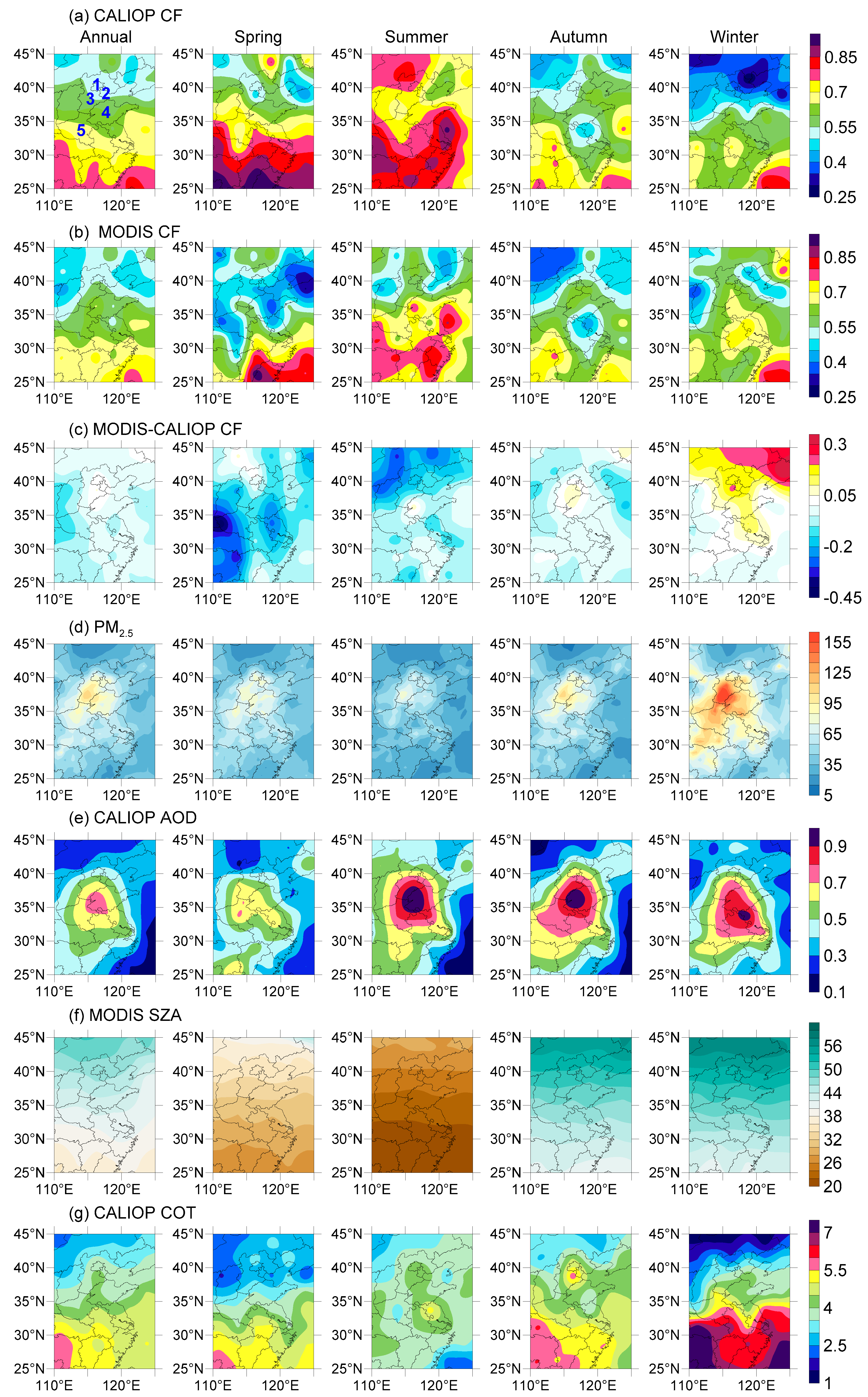
MODIS and CALIOP observed similar patterns for cloud fraction in Eastern China—the cloud fraction decreased from south to north (Figure 9a,b). Both of them observed the highest cloud fraction over Eastern China in summer and over the southern region in spring. The CTH was the highest in summer and lowest in winter (Table 1). For the annual averaged cloud fraction, CALIOP was 0.04 higher than MODIS (Table 1).
Annually, MODIS observed more clouds in regions of central Eastern China (including Beijing-Tianjin-Hebei-Shandong-Henan) and the northeastern corner (Figure 9c), which may be due to the high PM2.5 (Figure 9d), high AOD (Figure 9e), and high SZA (Figure 9f).
In spring and summer, CALIOP observed more clouds than MODIS due to the low COT (Figure 9g), which is consistent with clouds detected by CALIOP but not by MODIS having a low COT (Figure 2f). The averaged cloud fraction of CALIOP is 0.13 and 0.11 higher than that of MODIS, and the averaged CTH of CALIOP is 2.28 km and 0.87 km higher than that of MODIS in spring and summer, respectively. That may be caused by MODIS not observing clouds detected by CALIOP with a higher CTH (Figure 2c) and lower COT (Figure 2f).
The distribution of the annual cloud fraction difference is similar to that in autumn and particularly in winter (Figure 9c). In autumn and particularly in winter, the haze pollution in the center of Eastern China and the high SZA in the north may induce MODIS to observe more clouds than CALIOP. Both haze pollution and high SZA in the northeastern corner caused MODIS to observe more clouds than CALIOP there. The averaged MODIS cloud fraction over the whole of Eastern China is 0.08 higher than the CALIOP-observed cloud fraction in winter (Table 1). The MODIS CTH was very low in winter (3.66 km) due to its misclassification of aerosols as clouds; it is 2.17 km lower than CALIOP CTH (Table 1).
4. Conclusions
In this study, we investigated how cloud detection from MODIS cloud mask products performs over Eastern China during 2013–2016 in comparison with observations from CALIOP. Our analysis illustrated that, on average, MODIS and CALIOP were in agreement 82% of the time. Most of the discrepancies were associated with low MODIS CTH (<1.5 km) and low CALIOP COT (<0.4). MODIS observations of clouds undetected by CALIOP were due to a high aerosol optical depth and high solar zenith angle. The ratio of MODIS cloud pixel numbers to CALIOP cloud-free pixel numbers increased largely with an increase in AOD and SZA (2–4 times for AOD and 4–21 times for SZA over different surfaces), indicating that high aerosol load and high SZA may contaminate MODIS cloud detection. CALIOP observed more clouds with a COT less than 0.4 than MODIS, and about 62% of the clouds observed by CALIOP and undetected by MODIS had a COT less than 0.4. That suggested that CALIOP was better at detecting optically thin clouds than MODIS.
In addition, the consistent proportion observed by both MODIS and CALIOP was the largest for ice clouds. The cloud detection difference between MODIS and CALIOP was mainly ascribed to water clouds, and undetermined-phase clouds contributed the second-most to this difference. Low clouds (Cu and Sc) contributed most of the discrepancies for all surfaces, which is consistent with most of the discrepancies being associated with a low MODIS CTH.
Author Contributions
S.T. and G.S. conceived and designed the study; X.Z. performed the calculations and analyses; S.T. wrote the paper; S.T. and X.Z. prepared the figures.
Funding
This research was funded by the National Natural Science Foundation of China (grant No. 41590874) and International Partnership Program of Chinese Academy of Sciences (grant No. 134111KYSB20180021).
Acknowledgments
The authors thank China National Environmental Monitoring Center for providing air quality data, Level 1 and Atmosphere Archive and Distribution System (LAADS) of the NASA Goddard Space Flight Center for providing MODIS data, and NASA Langley Research Center Atmospheric Science Data Center for providing CALIPSO data.
Conflicts of Interest
The authors declare no conflict of interest.
References
- Ramanathan, V.; Cess, R.D.; Harrison, E.F.; Minnis, P.; Barkstrom, B.R.; Ahmad, E.; Hartmann, D. Cloud-radiative forcing and climate: Results from the earth radiation budget experiment. Science 1989, 243, 57–63. [Google Scholar] [CrossRef] [PubMed]
- Trenberth, K.E.; Fasullo, J.T.; Kiehl, J. Earth’s global energy budget. Bull. Am. Meteorol. Soc. 2009, 90, 311–323. [Google Scholar] [CrossRef]
- Koren, I.; Martins, J.V.; Remer, L.A.; Afargan, H. Smoke invigoration versus inhibition of clouds over the amazon. Science 2008, 321, 946–949. [Google Scholar] [CrossRef] [PubMed]
- Bony, S.; Stevens, B.; Frierson, D.M.W.; Jakob, C.; Kageyama, M.; Pincus, R.; Shepherd, T.G.; Sherwood, S.C.; Siebesma, A.P.; Sobel, A.H.; et al. Clouds, circulation and climate sensitivity. Nat. Geosci. 2015, 8, 261–268. [Google Scholar] [CrossRef]
- Jing, X.; Zhang, H.; Satoh, M.; Zhao, S. Improving representation of tropical cloud overlap in GCMs based on cloud-resolving model data. J. Meteorol. Res. 2018, 32, 233–245. [Google Scholar] [CrossRef]
- Li, C.; Ma, J.; Yang, P.; Li, Z. Detection of cloud cover using dynamic thresholds and radiative transfer models from the polarization satellite image. J. Quant. Spectrosc. Radiat. Transf. 2019, 222, 196–214. [Google Scholar] [CrossRef]
- Latham, J.; Rasch, P.; Chen, C.-C.; Kettles, L.; Gadian, A.; Gettelman, A.; Morrison, H.; Bower, K.; Choularton, T. Global temperature stabilization via controlled albedo enhancement of low-level maritime clouds. Philos. Trans. R. Soc. A Math. Phys. Eng. Sci. 2008, 366, 3969–3987. [Google Scholar]
- Kambezidis, H.D.; Kaskaoutis, D.G.; Kalliampakos, G.K.; Rashki, A.; Wild, M. The solar dimming/brightening effect over the Mediterranean basin in the period 1979–2012. J. Atmos. Sol. Terr. Phys. 2016, 150, 31–46. [Google Scholar] [CrossRef]
- Longman, R.J.; Giambelluca, T.W.; Alliss, R.J.; Barnes, M.L. Temporal solar radiation change at high elevations in Hawai’i. J. Geophys. Res. Atmos. 2014, 119, 6022–6033. [Google Scholar] [CrossRef]
- Badarinath, K.V.S.; Sharma, A.R.; Kaskaoutis, D.G.; Kharol, S.K.; Kambezidis, H.D. Solar dimming over the tropical urban region of Hyderabad, India: Effect of increased cloudiness and increased anthropogenic aerosols. J. Geophys. Res. Atmos. 2010, 115, D21208. [Google Scholar] [CrossRef]
- Stephens, G.L.; Vane, D.G.; Boain, R.J.; Mace, G.G.; Sassen, K.; Wang, Z.; Illingworth, A.J.; O’Connor, E.J.; Rossow, W.B.; Durden, S.L.; et al. The cloudsat mission and the a-train. Bull. Am. Meteorol. Soc. 2002, 83, 1771–1790. [Google Scholar] [CrossRef]
- Ackerman, S.A.; Strabala, K.I.; Menzel, W.P.; Frey, R.A.; Moeller, C.C.; Gumley, L.E. Discriminating clear sky from clouds with MODIS. J. Geophys. Res. Atmos. 1998, 103, 32141–32157. [Google Scholar] [CrossRef]
- Ackerman, S.; Frey, R.; Strabala, K.; Liu, Y.; Gumley, L.; Baum, B.; Menzel, P. Discriminating Clear-Sky from Cloud with Modis: Algorithm Theoretical Basis Document (mod35); Version 6.1; Cooperative Institute for Meteorological Satellite Studies, University of Wisconsin-Madison: Madison, WI, USA, 2010. [Google Scholar]
- Platnick, S.; King, M.D.; Ackerman, S.A.; Menzel, W.P.; Baum, B.A.; Riedi, J.C.; Frey, R.A. The MODIS cloud products: Algorithms and examples from terra. IEEE Trans. Geosci. Remote Sens. 2003, 41, 459–473. [Google Scholar] [CrossRef]
- Winker, D.M.; Vaughan, M.A.; Omar, A.; Hu, Y.; Powell, K.A.; Liu, Z.; Hunt, W.H.; Young, S.A. Overview of the Calipso mission and Caliop data processing algorithms. J. Atmos. Ocean. Technol. 2009, 26, 2310–2323. [Google Scholar] [CrossRef]
- Winker, D.M.; Pelon, J.; Coakley, J.A.C., Jr.; Ackerman, S.A.; Charlson, R.J.; Colarco, P.R.; Flamant, P.; Fu, Q.; Hoff, R.M.; Kittaka, C.; et al. The Calipso mission: A global 3d view of aerosols and clouds. Bull. Am. Meteorol. Soc. 2010, 91, 1211–1230. [Google Scholar] [CrossRef]
- Holz, R.E.; Ackerman, S.A.; Nagle, F.W.; Frey, R.; Dutcher, S.; Kuehn, R.E.; Vaughan, M.A.; Baum, B. Global moderate resolution imaging spectroradiometer (MODIS) cloud detection and height evaluation using caliop. J. Geophys. Res. Atmos. 2008, 113, D00A19. [Google Scholar] [CrossRef]
- Delanoë, J.; Hogan, R.J. Combined Cloudsat-Calipso-MODIS retrievals of the properties of ice clouds. J. Geophys. Res. Atmos. 2010, 115. [Google Scholar] [CrossRef]
- Hirakata, M.; Okamoto, H.; Hagihara, Y.; Hayasaka, T.; Oki, R. Comparison of global and seasonal characteristics of cloud phase and horizontal ice plates derived from Calipso with MODIS and ECMWF. J. Atmos. Ocean. Technol. 2014, 31, 2114–2130. [Google Scholar] [CrossRef]
- Holz, R.E.; Platnick, S.; Meyer, K.; Vaughan, M.; Heidinger, A.; Yang, P.; Wind, G.; Dutcher, S.; Ackerman, S.; Amarasinghe, N.; et al. Resolving ice cloud optical thickness biases between Caliop and MODIS using infrared retrievals. Atmos. Chem. Phys. 2016, 16, 5075–5090. [Google Scholar] [CrossRef]
- Shang, H.; Chen, L.; Tao, J.; Su, L.; Jia, S. Synergetic use of modis cloud parameters for distinguishing high aerosol loadings from clouds over the north china plain. IEEE J. Sel. Top. Appl. Earth Obs. Remote Sens. 2014, 7, 4879–4886. [Google Scholar] [CrossRef]
- Mao, F.; Duan, M.; Min, Q.; Gong, W.; Pan, Z.; Liu, G. Investigating the impact of haze on modis cloud detection. J. Geophys. Res. Atmos. 2015, 120, 12237–12247. [Google Scholar] [CrossRef]
- Tan, S.-C.; Zhang, X.; Wang, H.; Chen, B.; Shi, G.-Y.; Shi, C. Comparisons of cloud detection among four satellite sensors on severe haze days in eastern china. Atmos. Ocean. Sci. Lett. 2018, 11, 86–93. [Google Scholar] [CrossRef]
- Zhang, X.; Tan, S.-C.; Shi, G.-Y.; Wang, H. Improvement of MODIS cloud mask over severe polluted eastern china. Sci. Total Environ. 2019, 654, 345–355. [Google Scholar] [CrossRef] [PubMed]
- Wang, H.; Tan, S.-C.; Wang, Y.; Jiang, C.; Shi, G.-Y.; Zhang, M.-X.; Che, H.-Z. A multisource observation study of the severe prolonged regional haze episode over eastern china in January 2013. Atmos. Environ. 2014, 89, 807–815. [Google Scholar] [CrossRef]
- Wang, H.; Shi, G.Y.; Zhang, X.Y.; Gong, S.L.; Tan, S.C.; Chen, B.; Che, H.Z.; Li, T. Mesoscale modelling study of the interactions between aerosols and PBL meteorology during a haze episode in China Jing–Jin–Ji and its near surrounding region—Part 2: Aerosols’ radiative feedback effects. Atmos. Chem. Phys. 2015, 15, 3277–3287. [Google Scholar] [CrossRef]
- Wu, P.; Ding, Y.; Liu, Y. Atmospheric circulation and dynamic mechanism for persistent haze events in the Beijing–Tianjin–Hebei region. Adv. Atmos. Sci. 2017, 34, 429–440. [Google Scholar] [CrossRef]
- Huang, J.; Minnis, P.; Chen, B.; Huang, Z.; Liu, Z.; Zhao, Q.; Yi, Y.; Ayers, J.K. Long-range transport and vertical structure of Asian dust from Calipso and surface measurements during Pacdex. J. Geophys. Res. Atmos. 2008, 113. [Google Scholar] [CrossRef]
- Tan, S.-C.; Shi, G.-Y.; Wang, H. Long-range transport of spring dust storms in inner Mongolia and impact on the china seas. Atmos. Environ. 2012, 46, 299–308. [Google Scholar] [CrossRef]
- Wang, X.; Liu, J.; Che, H.; Ji, F.; Liu, J. Spatial and temporal evolution of natural and anthropogenic dust events over northern china. Sci. Rep. 2018, 8, 2141. [Google Scholar] [CrossRef]
- Baum, B.A.; Menzel, W.P.; Frey, R.A.; Tobin, D.C.; Holz, R.E.; Ackerman, S.A.; Heidinger, A.K.; Yang, P. Modis cloud-top property refinements for collection 6. J. Appl. Meteorol. Climatol. 2012, 51, 1145–1163. [Google Scholar] [CrossRef]
- Rossow, W.B.; Walker, A.W.; Beuschel, D.E.; Roiter, M.D. International Satellite Cloud Climatology Project (ISCCP) Documentation of New Cloud Datasets; WMO/TD-NO. 737; World Meteorological Organization: Geneva, Switzerland, 1996. [Google Scholar]
- King, M.D.; Platnick, S.; Menzel, W.P.; Ackerman, S.A.; Hubanks, P.A. Spatial and temporal distribution of clouds observed by MODIS onboard the terra and aqua satellites. IEEE Trans. Geosci. Remote Sens. 2013, 51, 3826–3852. [Google Scholar] [CrossRef]
- Grosvenor, D.P.; Wood, R. The effect of solar zenith angle on MODIS cloud optical and microphysical retrievals within marine liquid water clouds. Atmos. Chem. Phys. 2014, 14, 7291–7321. [Google Scholar] [CrossRef] [Green Version]
- Zhang, X.; Tan, S.; Shi, G. Comparison between MODIS-derived day and night cloud cover and surface observations over the north china plain. Adv. Atmos. Sci. 2018, 35, 146–157. [Google Scholar] [CrossRef]
Figure 1.
The research region of Eastern China. Green, yellow, and blue backgrounds show dark, bright, and water surfaces on May 29, 2015, respectively. Red dots are environmental monitoring stations.
Figure 1.
The research region of Eastern China. Green, yellow, and blue backgrounds show dark, bright, and water surfaces on May 29, 2015, respectively. Red dots are environmental monitoring stations.

Figure 2.
The histogram of total pixel numbers of consistent and non-consistent Moderate Resolution Imaging Spectroradiometer (MODIS) and Cloud–Aerosol Lidar with Orthogonal Polarization (CALIOP) cloud detection over dark, bright, and water surfaces along with (a) MODIS cloud top height (CTH); (b) MODIS cloud optical thickness (COT); (c) CALIOP CTH; (d) CALIOP cloud base height (CBH); (e) CALIOP cloud thickness; and (f) CALIOP COT. Gray and purple groups are consistent and non-consistent observations, respectively. Numbers shown on each panel are total pixel numbers.

Figure 3.
The r_MODalone as a function of solar zenith angle (SZA) and MODIS cloud top height (CTH) over (a) dark, (b) bright, and (c) water surfaces, and the r_CALalone as a function of SZA and CALIOP CTH over (d) dark, (e) bright, and (f) water surfaces.
Figure 3.
The r_MODalone as a function of solar zenith angle (SZA) and MODIS cloud top height (CTH) over (a) dark, (b) bright, and (c) water surfaces, and the r_CALalone as a function of SZA and CALIOP CTH over (d) dark, (e) bright, and (f) water surfaces.

Figure 4.
Dependence of r_MODcloud_CALfree on aerosol optical depth (AOD) and solar zenith angle (SZA) over (a) dark; (b) bright; and (c) water surfaces.
Figure 4.
Dependence of r_MODcloud_CALfree on aerosol optical depth (AOD) and solar zenith angle (SZA) over (a) dark; (b) bright; and (c) water surfaces.

Figure 5.
Variations in r_MODcloud_CALfree with (a) AOD and (b) SZA, and (c) variations in r_CALcloud_MODfree with COT.
Figure 5.
Variations in r_MODcloud_CALfree with (a) AOD and (b) SZA, and (c) variations in r_CALcloud_MODfree with COT.

Figure 6.
(a) The proportion of MODIS cloud phases (water cloud, ice cloud, and undetermined-phase cloud); (b–d) The proportion of water, ice, and undetermined-phase clouds over dark, bright, and water surfaces, respectively. Solid lines show the consistent proportion observed by both MODIS and CALIOP, and dashed lines show the non-consistent proportion observed by MODIS alone.

Figure 7.
The variation of the proportion of consistent (solid lines) and non-consistent (dashed lines) MODIS and CALIOP cloud detection data with AOD for different cloud types over (a) dark, (b) bright, and (c) water surfaces, respectively, and the variation of r_MODcloud_CALfree for each cloud type with AOD over (d) dark, (e) bright, and (f) water surfaces, respectively.

Figure 8.
The variation of the proportion of consistent (solid lines) and non-consistent (dashed lines) MODIS and CALIOP cloud detection with SZA for different cloud types over (a) dark, (b) bright, and (c) water surfaces, respectively, and the variation of r_MODcloud_CALfree for each cloud type with SZA over (d) dark, (e) bright, and (f) water surfaces, respectively.

Figure 9.
Annual and seasonal averages of (a) CALIOP cloud fraction (CF); (b) MODIS CF; (c) the CF difference between MODIS and CALIOP; (d) PM2.5 (μg m−3); (e) AOD; (f) SZA; and (g) COT. Each row shows different parameters, and each column shows different seasons. Locations 1–5 in (a) Annual show Beijing and Tianjin cities, and Hebei, Shandong, and Henan provinces.


Table 1.
MODIS and CALIOP averaged cloud fraction and CTH over Eastern China.
| Season | CALIOP Cloud Fraction | MODIS Cloud Fraction | CALIOP CTH (km) | MODIS CTH (km) |
|---|---|---|---|---|
| Annual | 0.64 | 0.60 | 7.35 | 5.58 |
| Spring | 0.70 | 0.57 | 8.47 | 6.19 |
| Summer | 0.77 | 0.66 | 8.85 | 7.98 |
| Autumn | 0.59 | 0.55 | 6.26 | 5.07 |
| Winter | 0.54 | 0.62 | 5.83 | 3.66 |
© 2019 by the authors. Licensee MDPI, Basel, Switzerland. This article is an open access article distributed under the terms and conditions of the Creative Commons Attribution (CC BY) license (http://creativecommons.org/licenses/by/4.0/).
Share and Cite
MDPI and ACS Style
Tan, S.; Zhang, X.; Shi, G. MODIS Cloud Detection Evaluation Using CALIOP over Polluted Eastern China. Atmosphere 2019, 10, 333. https://0-doi-org.brum.beds.ac.uk/10.3390/atmos10060333
AMA Style
Tan S, Zhang X, Shi G. MODIS Cloud Detection Evaluation Using CALIOP over Polluted Eastern China. Atmosphere. 2019; 10(6):333. https://0-doi-org.brum.beds.ac.uk/10.3390/atmos10060333
Chicago/Turabian StyleTan, Saichun, Xiao Zhang, and Guangyu Shi. 2019. "MODIS Cloud Detection Evaluation Using CALIOP over Polluted Eastern China" Atmosphere 10, no. 6: 333. https://0-doi-org.brum.beds.ac.uk/10.3390/atmos10060333
Note that from the first issue of 2016, this journal uses article numbers instead of page numbers. See further details here.