1. Introduction
Elevated levels of air pollution generated by the road traffic have been associated with severe illness such as the development of asthma in adults, impaired lung growth in children, and an increased risk of chronic obstructive pulmonary disease [
1]. Consequently, air quality in urban canyons needs to be improved to protect pedestrians, cyclists, and drivers from exposure to contaminants such as particulate matter (PM), volatile organic compounds (VOCs), carbon monoxide (CO), nitrogen oxides (NO
x), and sulfur dioxide (SO
2) that are primarily emitted from motor vehicles [
2]. Among these contaminants, NO
x and VOCs represent the most significant concern for air pollution in street canyons because they are released at very short distances from the receptors. Moreover, under the presence of sunlight, fast reactions occur between them leading to the formation of particulate matter and tropospheric ozone (O
3) which are very dangerous secondary pollutants [
3].
Various tools have been employed to measure the levels of contaminants inside the street canyons [
4], such as, field observations [
5,
6,
7], wind tunnels measurements [
8,
9], and several semi-empirical models including the ADMS-Urban dispersion model [
10], CALINE4 [
11], and the Urban Street Model [
12].
The technique utilized for this study was computational fluid dynamics (CFD) modeling because it helps to reduce the time required to optimize a physical model and is less expensive in comparison with wind tunnels. Moreover, the simulation of dispersion and boundary conditions with CFD are better studied [
13]. Additionally, recent advances in computer technology make CFD a powerful tool for air pollution modeling [
14,
15]; using CFD, the description of air flow patterns at the city-block scale with high spatial-resolution can be achieved [
16], and important simulations such as the influence of building geometry on wind flow and heat convection can be carried out [
17,
18].
In microscale environments, many factors such as vehicle emissions, street canyon configuration, surface heating, and chemical reactions are dynamically involved in the dispersion of pollutants. A number of studies have tried to model these factors using CFD. To evaluate surface heating, Kim and Baik [
19] systematically characterized two-dimensional flow regimes with the presence of street bottom heating, although failed to take heating of buildings into account. Xie et al. [
20] considered the impact of heating of three idealized sunlit wall configurations on pollutant dispersion in a two-dimensional computational domain perpendicular to the street canyon wind direction; later, Kim and Baik [
21] extended this work by examining the effects of street-bottom and building-roof heating on flow fields in a three-dimensional ideal urban canyon setting. This work highlighted the importance of including street-bottom and building roof heating in three-dimensional flow models. Bottillo et al. [
22] remarked on the effect of solar radiation in an urban street canyon with three-dimensional flow field under different ambient wind conditions, confirming the impact of the velocity on the heat transfer process.
Meanwhile, studies about the dispersion of reactive pollutants inside street canyon were conducted by Baker et al. [
23] using a simple NO–NO
2–O
3 photochemistry model to evaluate the isothermal dispersal and chemistry in and above the street canyons with an aspect ratio of 1. Baik et al. [
24] extended this work by showing, with a simple street canyon model and an aspect ratio of 1, the importance of the building surface radiation effects on the wind flow pattern in the urban areas when modeling reactive pollutant dispersion. In the following years, Kwak and Baik [
25] calculated the photochemical reaction of pollutants in and above an idealized street canyon using a two-dimensional CFD model coupled for the first time with a Carbon Bond Mechanism IV (CBM-IV) [
26]. Similarly, Kwak and Baik [
27] used an idealistic two-dimensional model with urban surface, radiation and chemical processes to focus on the diurnal variation of NO
x and O
3 exchange. This study also employs a CFD model coupled with a CBM-IV chemical model to represent reactive pollutants inside the street canyons.
Despite significant effort, there is still a lack of research in non-idealized three-dimensional environments which restricts the ability to simulate pollutant concentrations at the street level in complex urban areas. One of the main reasons for this is the specification of boundary conditions for realistic urban areas. Some authors have overcome this drawback by coupling mesoscale models with CFD simulations, for example, Baik et al. [
28] used a CFD model coupled to a mesoscale meteorological model to examine urban flow and pollutant dispersion in a densely built-up area of Seoul. Tewari et al. [
29] reported the benefits of coupling a microscale transport and dispersion model with a mesoscale numerical weather prediction model; significant improvements were observed when wind fields were produced by downscaling a meteorological model output as the initial and boundary CFD conditions. Recently, Kwak et al. [
30] developed an integrated three-dimensional model that coupled CFD with mesoscale meteorological and chemistry-transport models to simulate the air pollution from 09:00 to 18:00 local time in Seoul. In this work, the Weather Research and Forecasting model (WRF) [
31] and the Community Multiscale Air Quality model (CMAQ) [
32] are employed as mesoscale meteorological and air quality models to obtain boundary conditions for CFD.
This study is an ambitious attempt to evaluate the concentration of reactive pollutants in a realistic urban street canyon domain over 24 h by integrating a CFD model coupled with a chemical reaction model (CBM-IV), a radiation model, and boundary conditions from WRF-CMAQ. The first objective is to couple CFD with the chemical reaction model (CBM-IV) to describe urban dynamics with high resolution. The second is to validate the CFD-coupled chemical reaction model by comparing the numerical simulation results of a realistic urban street canyon against the observed data collected from monitoring stations situated near the roadside. The final objective is to assess the roadside pollutant dispersion in realistic city blocks with the CFD-coupled chemical reaction model.
This paper is structured as follows: in
Section 2, the numerical CFD model coupled with the CBM-IV model, the surface energy budget model of the ground, and the building envelope model are presented. All the simulation settings required for the modeling of a realistic urban canyon are given in
Section 3. In
Section 4, the results of the CFD-coupled chemical reaction model simulations are validated against the observed data and CMAQ-simulated data. Also in the same section, the wind flow patterns and distribution of NO, NO
2, and O
3 at 08:00, 12:00, 16:00, and 20:00 JST are discussed in detail. In the last section, the conclusions are presented.
2. CFD-Coupled Chemical Reaction Model
In this study, the dispersion of reactive pollutants in urban canyons is described by the equations of continuity (Equation (1)), momentum (Equations (2) and (3)), and scalar transport coupled with the CBM-IV chemical model (Equation (4)). Air is modeled as an incompressible viscous flow, and the buoyancy forces are treated with the Boussinesq approximation.
Momentum equation:
where
xi represents the
ith cartesian coordinates,
Ui is the
ith mean velocity component (m/s),
t is the time (s),
ρ is the air density (kg/m
3),
is the pressure (Pa) derivation from its reference value,
δij is the Kronecker delta,
ℊ is the gravitational acceleration (m/s
2),
is the temperature derivation from its reference value (=
T −
) (K),
is the reference temperature (K),
v is the kinematic viscosity of air (m
2/s),
Km is the eddy diffusivity of momentum (m
2/s), and
k is the turbulent kinetic energy (m
2/s
2).
Scalar transport equation coupled with CBM-IV model:
where
represents the mean concentration of
ith species in the air (ppm),
D is the molecular diffusivity of the species (m
2/s), and
is the eddy diffusivity of the species (m
2/s). The last term of the scalar transport equation represents the net chemical production rate of the species calculated by the CBM-IV model.
The turbulence model standard k-ε is employed in this study (Equations (5) and (6)).
Turbulent kinetic energy equation:
where
is an empirical constant,
ε is the dissipation rate (m
2/s
3).
Turbulent dissipation rate of energy equation:
where
and
represent empirical constants.
Moreover, the energy equation (Equation (7)) is used to evaluate the influence of the radiation on the flow pattern and dispersion of pollutants.
Energy equation:
where
T represents the mean temperature (K),
is the dispersion by molecular motion (m
2/s),
is the dispersion by eddies (turbulence) (m
2/s) and
represents the source term of heat (W/m
2),
Cp is the specific heat at a constant pressure (J/kg/K), and
is the density of the air (kg/m
3). As part of this work, considerations about the influence of shortwave radiation (direct solar radiation) and longwave radiation (diffuse solar radiation) are taken into account by a surface energy budget model of the ground [
33] shown as follows:
where
is the ground albedo,
is shortwave radiation (W/m
2),
is Stefan–Boltzmann constant (W/m
2/K
4),
is the temperature of an element in the ground surface (K),
is the sky view factor for element
i,
is downward longwave radiation (W/m
2),
is the view factor of each surface element
j from element
i,
is the temperature of surface
j (K),
H is the sensible heat flux (W/m
2), and
is the heat flux into the ground (W/m
2). In Equation (8), the emissivity for longwave radiation is omitted because it is assumed to be 1 for all surfaces.
Similarly, a slightly modified building envelope model [
34] accounted for the radiation received in the air from the walls and roof surfaces of buildings (Equation (9)).
where
is the building surface albedo,
is the temperature of the outer building wall (K),
is the specific heat at a constant pressure (J/kg/K),
is the bulk heat transfer coefficient (W/m
2K),
(K) is the temperature of air above
and
is heat flux from the building into the air (W/m
2).
The finite volume method is used to discretize all the equations. The first-order Euler method is utilized as the time discretization scheme and the power law scheme as the discretization scheme of the convection and diffusion terms in the governing equations. Moreover, the semi-implicit method for pressure-linked equations (SIMPLE) algorithm was employed as the pressure–velocity coupling algorithm [
35]. The solar radiation and view factor are calculated following the method of Ikejima et al. [
33].
3. Simulation Setup
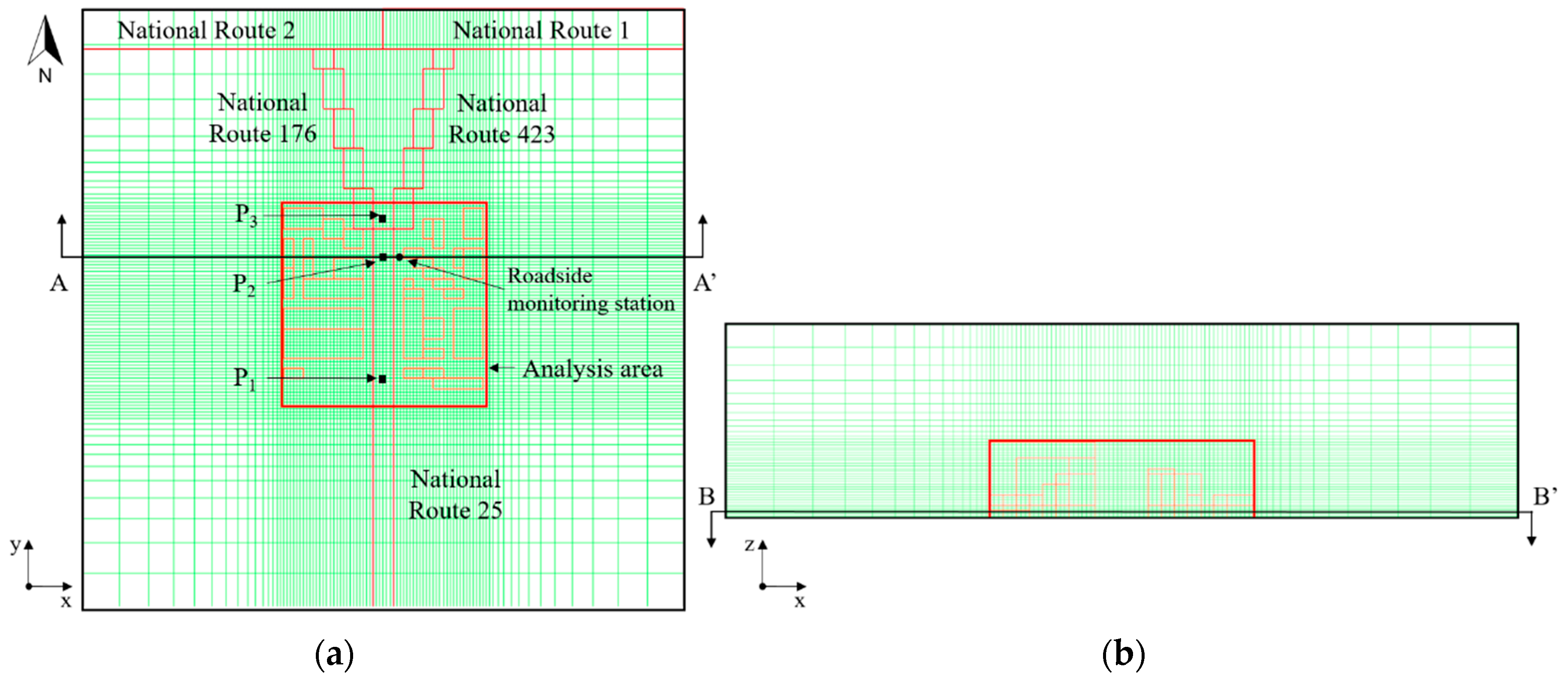
The three-dimensional CFD domain was set up in Umeda-Shinmichi (34.70° N, 135.50° E), Osaka City, Japan (
Figure 1a), where there is a typical urban street canyon layout with five roads flanked by twenty-two buildings (
Figure 1b). The information about the length, width, and height of every building was obtained by the results of the survey on land use conducted by Osaka City in 2005. The height of the array of buildings was from 12 to 48 m.
The size of the calculation domain was 600 m × 600 m × 150 m, and the analysis area was defined as 200 m × 200 m × 150 m, red square in
Figure 2a. The hexahedral mesh was 93 × 93 × 51 in the x-, y- and z-directions, respectively (
Figure 2), and a grid interval of 3.33 m in x- and y-direction was set.
The boundary conditions of the CFD domain for temperature, wind speed and wind direction, and those for air pollutant concentrations were obtained from results of meteorological simulations by WRF v3.7 (
Supplementary Material Figure S1) and air quality simulations by CMAQ v5.1 (
Supplementary Material Figure S2), respectively.
Supplementary Material Figure S3 and Table S1 correspondingly show modeling domains and configurations for the WRF-CMAQ simulation. The simulation was conducted over seven modeling domains from domain 1 (D1), covering East Asia with 64-km grids, to domain 7 (D7), covering Osaka Prefecture with 1-km grids, for a period from 24 June to 31 August 2010. The vertical domain consisted of 30 layers with the middle heights of the first, second, and third layers being 28 m, 92 m, and 190 m, respectively. The physics parameterizations and input data for WRF and the chemical mechanisms, including the Carbon Bond mechanism developed in 2005 (CB05) [
36], the next generation model of CBM-IV, for CMAQ were the same as those used by Shimadera et al. [
37]. Emission data for CMAQ were produced from the same datasets as those used by Uranishi et al. [
38], including the Japan Auto-Oil Program Emission Inventory-Data Base for vehicles (JEI-DB) in the year 2010 developed by the Japan Petroleum Energy Center [
39]. As shown in
Supplementary Material Figure S3, there are substantial NO
x emissions from vehicles, industrial areas, and large point sources in Osaka City.
23 August 2010 was chosen as the calculation date for the 24-h unsteady state CFD analysis because of the very clear and calm conditions so that photochemical reactions might play an essential role in air quality on the day. The WRF and CMAQ simulations in D7 on the day were compared with observed data by the Japan Meteorological Agency (JMA) at the Osaka Meteorological Observatory (34.68° N, 135.52° E) (
Supplementary Material Figure S3) and by the Ministry of the Environment of Japan (MOE) at Kokusetsu-Osaka station (34.68° N, 135.54° E) (
Supplementary Material Figure S3).
Figure 3 shows diurnal variations of the observed and WRF-simulated ground-level air temperature, wind speed and direction at the Osaka Meteorological Observatory, which is located 2 km southeast of Umeda-Shinmichi, on 23 August. The WRF-simulated air temperature agreed reasonably well with the observed data, showing a Root Mean Square Error (RMSE) value of 0.48 °C. The model also approximately captured the temporal variation of wind speed with a slight overestimation, indicated with a RMSE of 0.71 m/s. Both in the observation and WRF simulation, the wind direction mainly ranged from southwest to west, except at 08:00 and 09:00 JST (UTC+9) in the observation under calm conditions. For the case of the wind direction, the RMSE was 43 degrees.
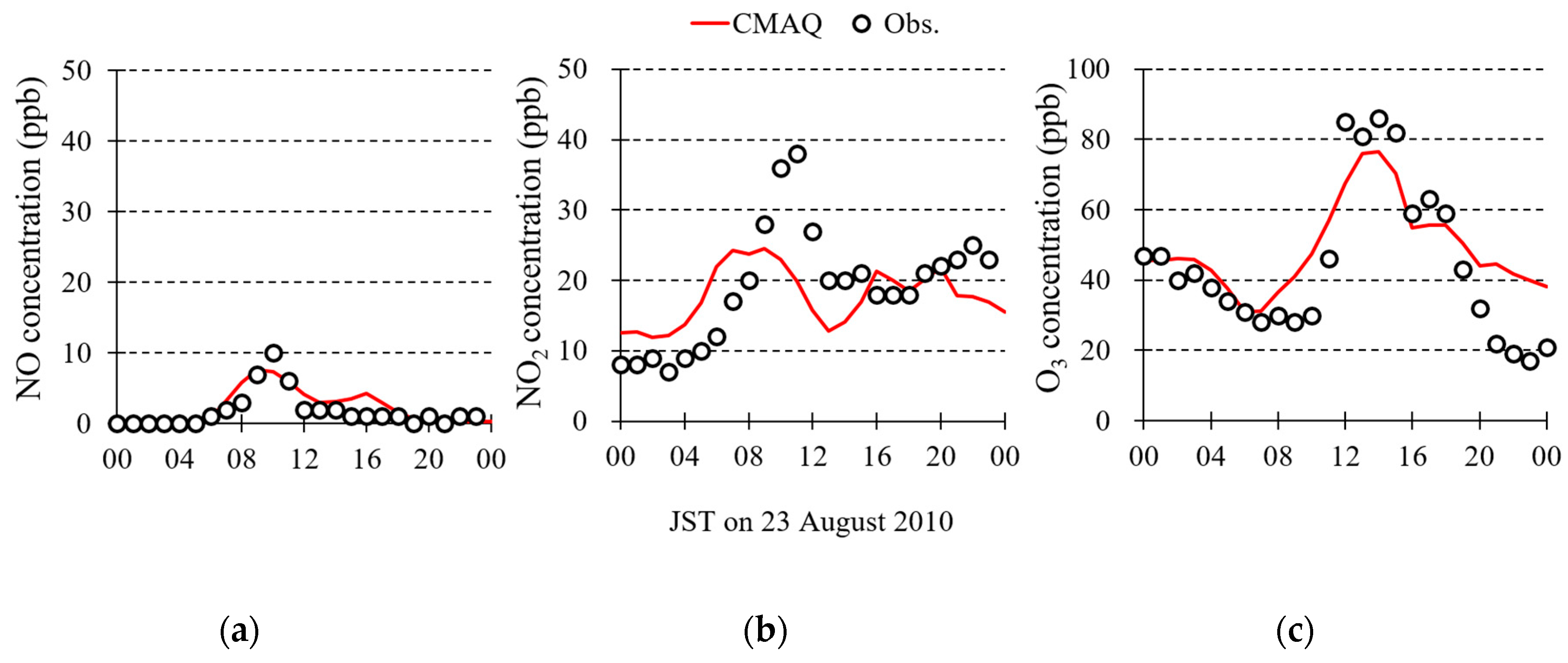
Figure 4 shows the diurnal variation of observed and CMAQ-simulated ambient concentrations of NO, NO
2, and O
3 at the Kokusetsu-Osaka station, which is located 4 km east-southeast of Umeda-Shinmichi. CMAQ approximately captured the variations and magnitudes of ambient concentrations of these air pollutants, except for NO
2 which was underestimated during the daytime. The RMSE of the NO, NO
2, and O
3 were 1.39 ppb, 7.03 ppb, and 11.43 ppb, respectively. These results indicate that WRF-CMAQ successfully produced meteorological and concentration fields around the study area for the CFD boundary conditions.
Because of the coarser vertical resolution of the WRF-CMAQ model compared with CFD, Monin–Obukhov Similarity Theory (MOST) was employed to determine the boundary vertical distribution of air temperature and wind components. Under MOST, the WRF-CMAQ data at heights 28 m and 92 m of Umeda-Shinmichi in D7 were used with a roughness length of 0.1 m. Moreover, the concentration under 28 m was the same value as the data at 28 m, and over 28 m the values were interpolated linearly. Because CB05 used in CMAQ has more species of VOCs than CBM-IV used in CFD, VOC species in CMAQ output were lumped into those in CBM-IV. Once this data was obtained, the vertical distribution from WRF-CMAQ at every hour and the values interpolated linearly in between each hour, the boundary conditions at transient state were set for the CFD model.
The emission rate from vehicles used as CMAQ input data was derived from JEI-DB with a horizontal resolution of 1 km × 1 km. The total emission rate from automobiles in the CFD domain was estimated from the JEI-DB data by multiplying the area ratio of the CFD domain to a grid of JEI-DB (0.36). Then, the total emission was allocated into the five national routes shown in
Figure 2 (National Route 1, National Route 2, National Route 176, National Route 423, National Route 25) by considering the traffic volume of each road provided by the Japan Ministry of Land, Infrastructure, Transport and Tourism [
40].
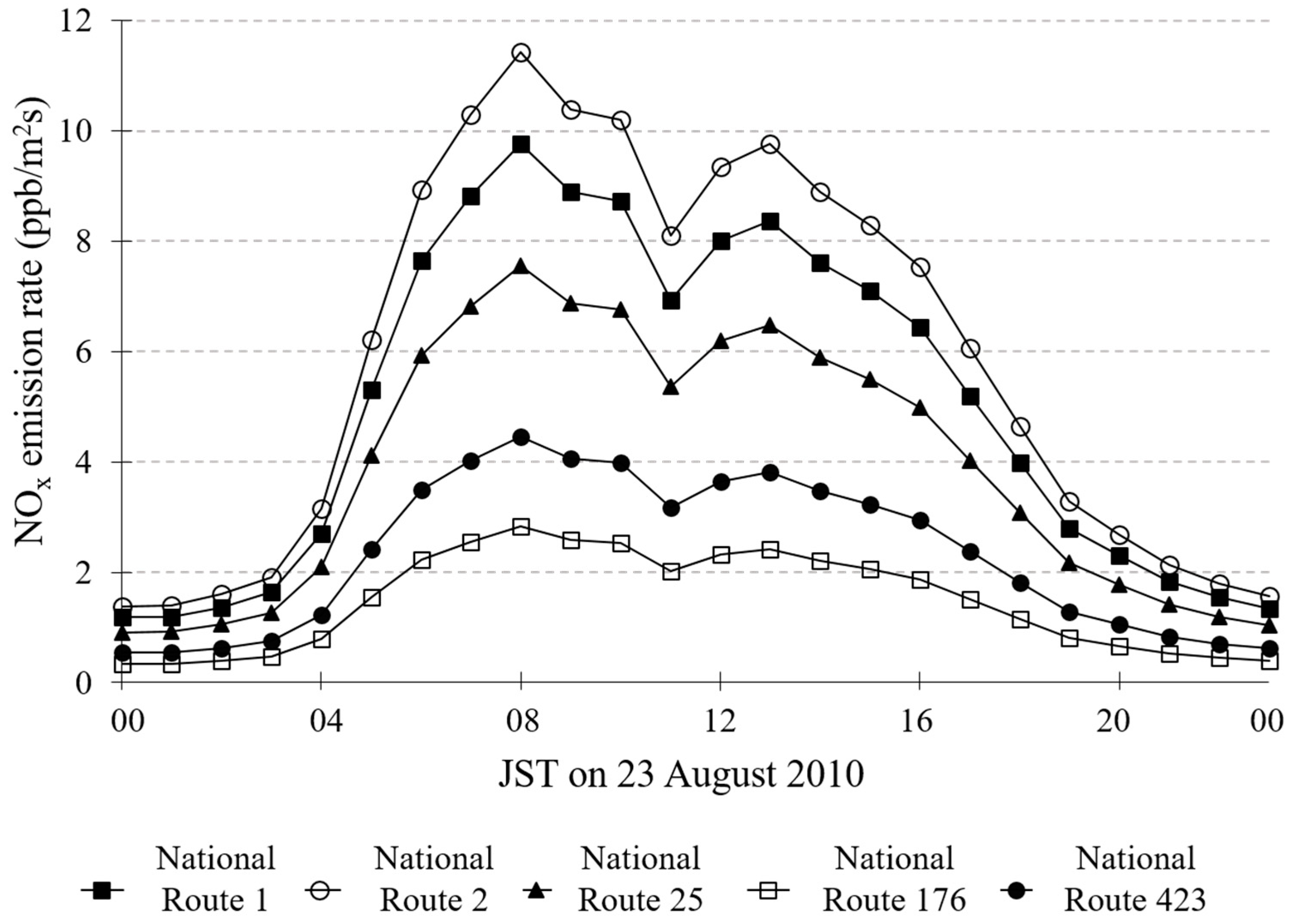
Figure 5 shows the diurnal variation of the NO
x (NO + NO
2) emission rate for 24 h for every national route. The average NO
2/NO
x emission ratio for the indicated area (0.36) was 0.1799. The information about the NO
x emission rate for every national route was used as the boundary condition for the emission rate and updated every hour in the CFD-coupled chemical reaction model. As discussed above, models of 24 h are mandatory since rush hours represent the peak emission rates.
4. Results and Discussion
The dispersion of pollutants inside urban street canyons is a phenomenon heavily reliant on the building geometry and roadside emissions. Therefore, it is quite challenging to capture the local aspects in mesoscale simulations softwares, such as WRF or CMAQ, because low model resolution cannot be well characterized [
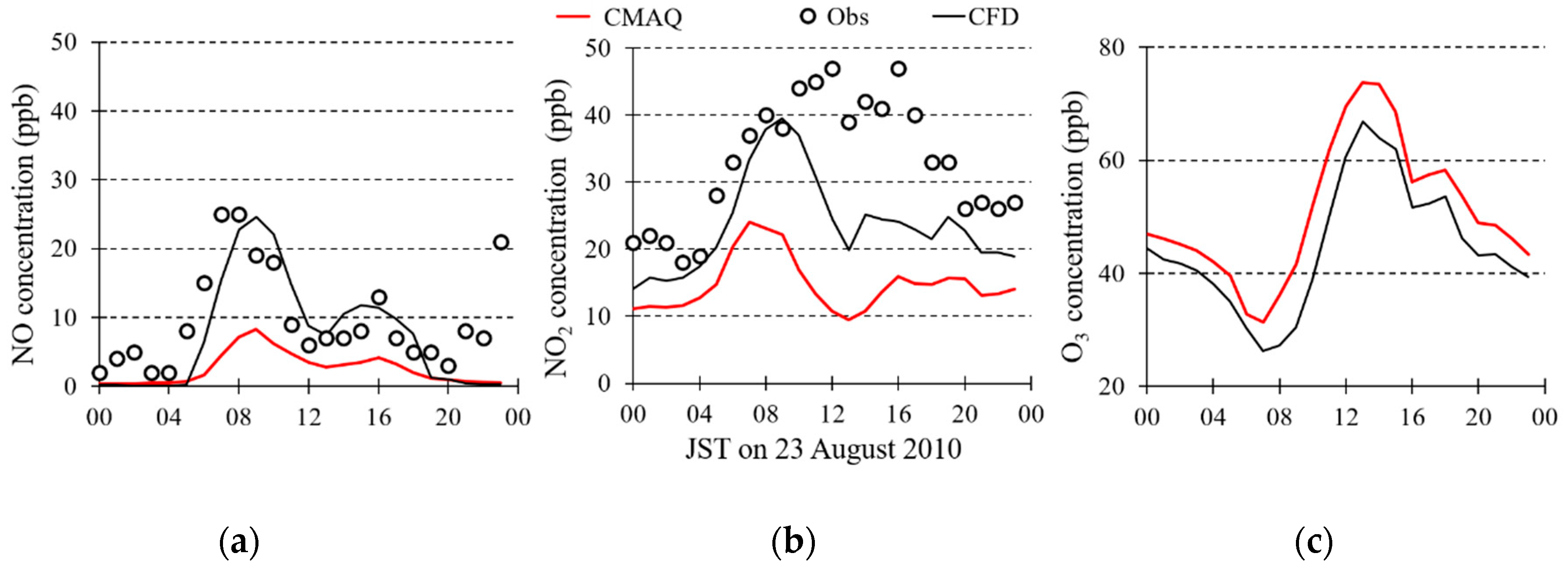
41]. In
Figure 6, the validation of the CFD model coupled chemical reaction model (CBM-IV) against CMAQ-simulated and the roadside monitoring station data by the Atmospheric Environmental Regional Observation System (AEROS) at Umeda-Shinmichi station (34.69° N, 135.50° E) about the diurnal variations of NO and NO
2 on 23 August 2010, is shown. For the case of O
3 in
Figure 6c, the comparison is only made between CMAQ and CFD simulations since the roadside monitoring station did not record the data for Ozone.
The RMSE in the case of the CFD-simulated results for NO and NO
2 were 6.35 ppb and 11.44 ppb, however, for the CMAQ-simulated results the values of the RMSE were 9.08 ppb and 20.35 ppb, respectively. Compared with CMAQ-simulated results, CFD-coupled chemical reaction model is more accurate describing the NO and NO
2 concentrations. The NO levels from the CFD calculation behaved almost identical to the observed data. As it is shown, there are some underestimations in NO
2 concentration from 09:00 JST to 18:00 JST, most likely because of the underestimation of the daytime background concentration indicated in
Figure 4. The O
3 concentrations output from CMAQ and CFD simulations show similar behavior, however the CFD simulations show consistently lower concentration. The results of this validation indicate how important it is to study particular emissions, the reactions in the modeling of air pollution, and the actual configuration of the urban street canyon using coupled CFD and chemical reaction modeling.
The behavior of NO, NO
2, and O
3 inside the analysis area, where the main road, National Route 25, runs perpendicular to the wind inflow with a width of 20 m, and sidewalks of 10 m at both sides was investigated (
Figure 2). The emission line source was placed in the middle of National Route 25 with a width of 20 m and a height of 1 meter from the ground.
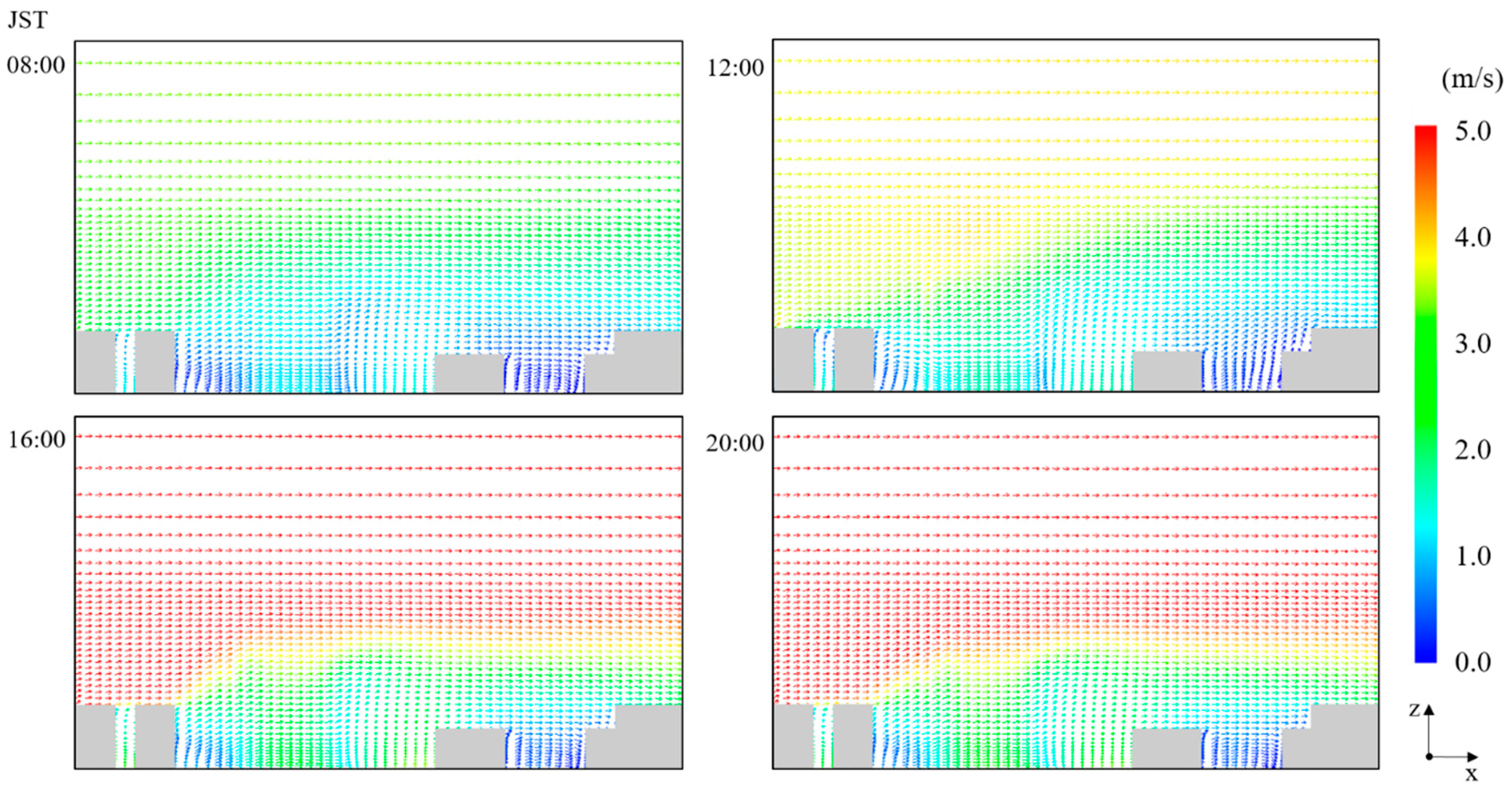
Figure 7 shows the airflow pattern in the analysis area at 08:00, 12:00, 16:00, and 20:00 JST in cross-section B-B’ (
Figure 2b). The height of z = 1.5 m is the same height as the monitoring station at which the data was compared. The flow field in
Figure 7 indicates a wind circulation restriction behind buildings typically present in street canyons. Throughout the day the inlet wind direction was sustained from west to east, and from afternoon (16:00 JST) until nighttime (20:00 JST) when the velocity reached maximum levels. Inside the street canyon (National Route 25), the wind flow moved mainly from south to north through the entire street canyon because of open space in the southwest part of the analysis area. Moreover, counterclockwise vortices developed on the road at 08:00, 12:00, 16:00, and 20:00 JST behind the buildings on the left side of the road, as result of the wind that speeded up and went through the channels between constructions. At noon, a shift in the wind flow in the superior side of the analysis area from west to east was observed, creating more vortices between buildings located downstream. Additionally,
Figure 7 demonstrates the importance of three-dimensional analyses since some eddies are seen at buildings corners where shear stresses are common and responsible for some turbulence in the flow.
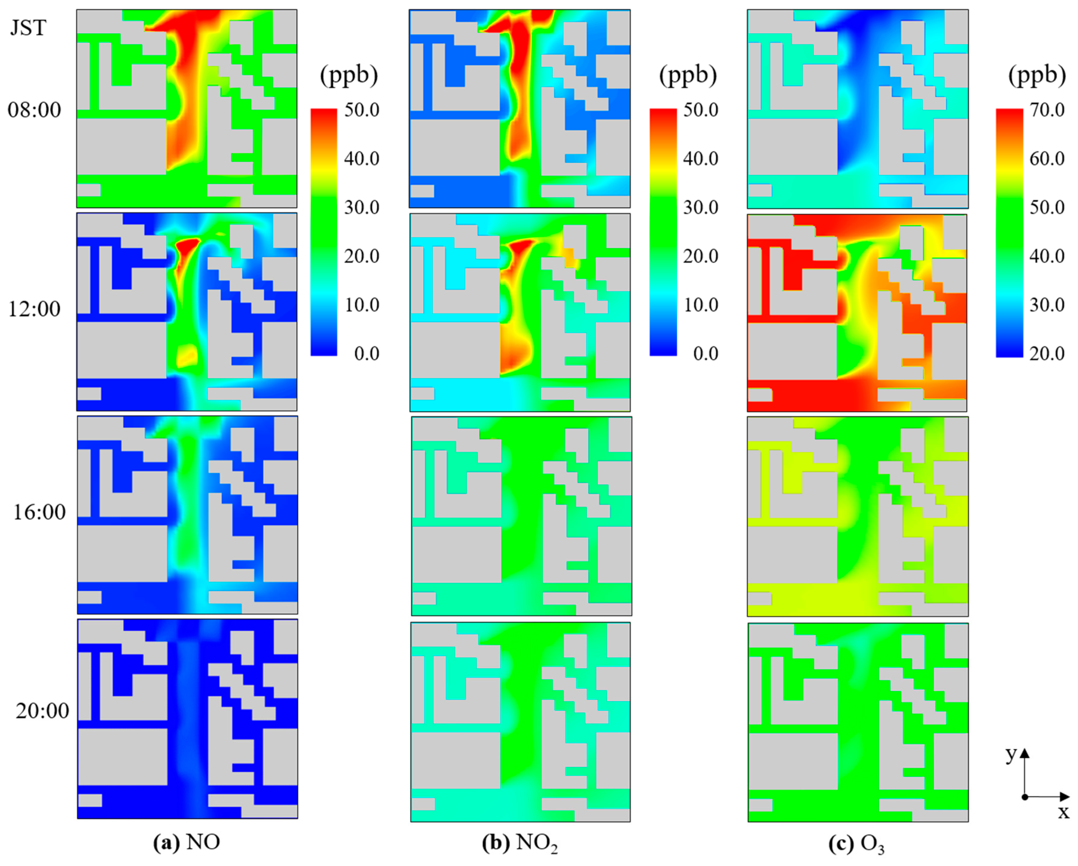
Figure 8 shows the spatial distribution of NO, NO
2, and O
3 concentrations at 08:00, 12:00, 16:00, and 20:00 JST in cross-section B-B’ (
Figure 2b). High levels of NO and NO
2 remained in the middle of the street canyon because building configurations do not allow their removal. During the day, the behavior of the contaminants changes depending on the emission rates and wind velocity. During the morning rush hours (07:00–09:00 JST), the NO
x concentration in the street canyon increases (
Figure 5) and stays on the street from 08:00 JST until 12:00 JST, especially behind the buildings where vortices are observed (
Figure 7). At 16:00 JST, the vehicle emission rate decreases, and the wind speed is higher, so the NO
2 concentrations reduced. However, at 20:00 JST, some slight concentration of NO
2 is still observed because of the titration reaction between NO and O
3 [
42]. Throughout the day, it is observed in
Figure 6, a different distribution between O
3 and NO
2 due to the proximity of the traffic-related emission (NO) that leads to NO
x titration. Besides, it is shown in
Figure 8 that high levels of NO and NO
2 are located in the right superior quadrant at noon because of the shift of the wind direction observed in
Figure 7.
Figure 9 shows the airflow patterns at 08:00, 12:00, 16:00, and 20:00 JST in cross-section A-A’ (
Figure 2a). Weaker wind flow is seen on the leeward side of the buildings and stagnation of the flow is evident upwind which is characteristic of wind flow around the buildings [
43]. When the wind flow encounters the buildings the flow is separated and the wind speed decreases, depending on the magnitude of the wind speed the scale of the vortices changes when moving in the positive z-direction. For this lateral view (cross-section A-A’,
Figure 2a), isolated roughness flow is observed, however, some perturbation is induced because of the proximity of the buildings in the background of the cross-section A-A’.
As mentioned before, adequate characterization of the dispersion and reaction of pollutants inside a real street urban environment requires the modeling of the effects of buildings and ground heating. The results of the analysis of the influence of the temperature on the analysis area, in specific Point 1, Point 2, and Point 3 (
Figure 2a) are presented in the
Supplementary Material Figure S6. The analysis of the temperature profiles showed no considerable difference under and above the heights of the buildings (~30 m). Thus, the influence of air temperature on the transport of contaminants for this urban street layout was considered minimal and almost negligible in comparison with the wind flow.
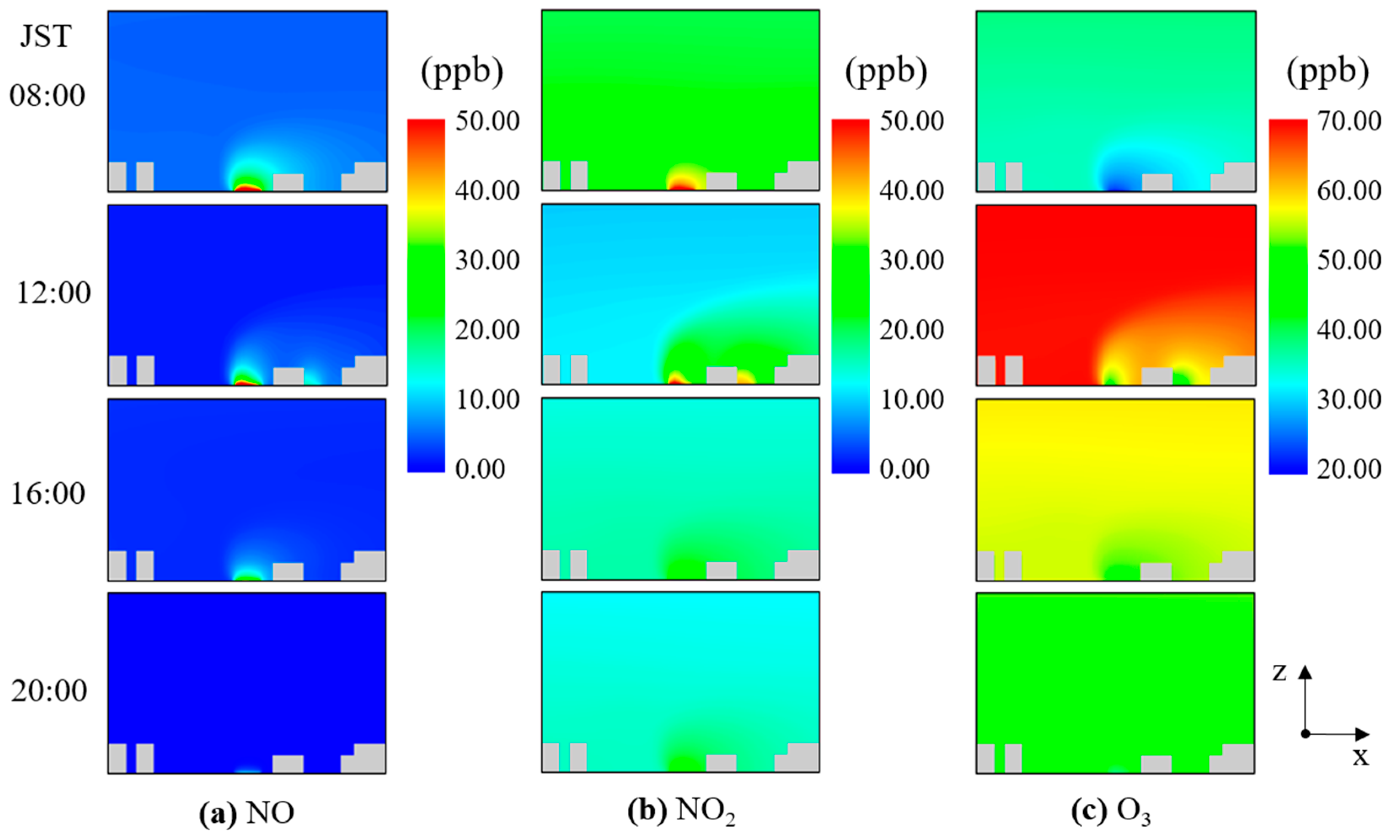
Figure 10 shows the spatial distribution of (a) NO, (b) NO
2, and (c) O
3 concentrations at 08:00, 12:00, 16:00, and 20:00 JST at cross-section A-A’ (
Figure 2a). Because of the vehicle exhaust located at a height of 1 meter in the middle of the analysis area, high NO and NO
2 concentrations remained near the surface level, mainly from 08:00 JST to 12:00 JST. The dispersion plume of NO, NO
2, and O
3 exhibits large vertical gradient from the ground to roof level of the building. As mentioned by Melkonyan and Kuttler [
44], NO and NO
2 enhance ozone’s dissociation and production, respectively. Thus, if the NO/NO
2 ratio decreases, ozone concentrations increase. In this study, all the National Routes studied showed high emission rates with a NO/NO
2 ratio of 4:1, suggesting that the NO
x titration was the main reason for the dissociation of O
3. At 20:00 JST, even when emissions from vehicles had decreased, the NO
2 concentration in the street was still present in contrast with the concentration above roof level. The vertical exchange of air pollutants is, therefore, shown to be mainly influenced by the vehicle emissions and building features.
5. Conclusions
This paper investigated the behavior of reactive pollutants inside a realistic urban street canyon by coupling a CFD model with a chemical reaction model (CBM-IV). The complexity of the urban street canyon geometry was represented by the CFD model and the dynamical mechanism involved in the dispersion of the pollutants were incorporated using mesoscale and radiation models. The spatial distribution of the reactive pollutants, in particular, NO, NO2, and O3 were researched over a 24-h period on 23 August 2010. The dispersion of the contaminants was highly dependent on the reaction processes, boundary conditions, and emission rates all integrated at the same time within the urban street canyon. The production of NOx or fading of O3 were especially found in regions with low wind speed and high turbulence, and NOx titration was noted to be of great importance. The O3 behavior was directly affected by the chemical reactions near the roadside, where fresh NO was being emitted, and was consequently controlled by the NOx distribution. The grid resolution of WRF-CMAQ appears to have a strong influence when representing the boundary conditions, and still, because of their limitations (1 km × 1 km minimum grid size) the particularities that accompany urban areas such as street, highways, unequal height of buildings, sidewalks cannot be well represented.
Finally, we can conclude that the prevailing wind flow mainly carried the air pollutants in the windward direction with small vortices recirculating pollutants inside the street canyon. This work is an intent to find better representations of boundary conditions and to step forward in the incorporation of radiation models and reactive models with the purpose of simulating urban-like environments, satisfactorily. Further efforts in this kind of research are necessary to reproduce the realities of the urban areas and the implications that it may have on the people who are exposed to these concentrations during the day.


