Modelling Canopy Actual Transpiration in the Boreal Forest with Reduced Error Propagation


1
Geomatics Engineering, Schulich School of Engineering, University of Calgary, 2500 University Drive NW, Calgary, AB T2N 1N4, Canada
2
Mechanical Engineering, University of Victoria, P.O. Box 1700 STN CSC, Victoria, BC V8P 5C2, Canada
*
Author to whom correspondence should be addressed.
Atmosphere 2020, 11(11), 1158; https://0-doi-org.brum.beds.ac.uk/10.3390/atmos11111158
Submission received: 5 September 2020
/
Revised: 16 October 2020
/
Accepted: 22 October 2020
/
Published: 27 October 2020
(This article belongs to the Special Issue Plant Adaptation to Global Climate Change)
Abstract
:The authors have developed a scaling approach to aggregate tree sap flux with reduced error propagation in modeled estimates of actual transpiration () of three boreal species. The approach covers three scales: tree point, single tree trunk, and plot scale. Throughout the development of this approach the error propagated from one scale to the next was reduced by analyzing the main sources of error and exploring how some field and lab techniques, and mathematical modeling can potentially reduce the error on measured or estimated parameters. Field measurements of tree sap flux at the tree point scale are used to obtain canopy transpiration estimates at the plot scale in combination with allometric correlations of sapwood depth (measured microscopically and scaled to plots), sapwood area, and leaf area index. We compared the final estimates to actual evapotranspiration and actual transpiration calculated with the Penman–Monteith equation, and the modified Penman–Monteith equation, respectively, at the plot scale. The scaled canopy transpiration represented a significant fraction of the forest evapotranspiration, which was always greater than 70%. To understand climate change impacts in forested areas, more accurate actual transpiration estimates are necessary. We suggest our model as a suitable approach to obtain reliable estimates in forested areas with low tree diversity.
1. Introduction
Climate change is reflected in almost every ecosystem by rising temperatures and changing precipitation patterns [1]. Higher seasonal temperatures in the boreal forest will increase evapotranspiration rates, decrease groundwater recharge, and affect water runoff levels [2,3,4]. Recent findings project a decrease in boreal forest biomass due to climate change, especially in the dominant conifer species [5], and these factors will likely change the boreal forest composition [6] and therefore change overall forest evapotranspiration. In vegetated areas, reliable water balance component estimates are of great importance for water management, sustainability, wildlife conservation, and nowadays, to understand and define plant species’ challenges to climate adaptation [7]. Evaporation and transpiration are two water balance components whose estimates are well known to carry uncertainty due to the use of equations and models that (1) lump the components into a single estimate of evapotranspiration (ET), and (2) focus on estimating ET under ideal atmospheric conditions and with an unlimited source of water (i.e., potential ET) [8,9]. This paper focuses on estimating actual transpiration () and actual ET () as a first step to reduce the uncertainty introduced by assumptions of ideal conditions. Recent studies have proven that modeling actual evapotranspiration and using site-specific calibrated variables greatly reduces the error and improves estimates of actual evapotranspiration [10,11].
Scaling a single tree’s point sap flow measurements to the watershed level is a complex and challenging task, not to mention the error propagated during the scaling process. Thus, most studies tend to focus on refining single components of the scaling process. For instance, direct ways to estimate actual transpiration of a single tree include the heat thermal dissipation method developed by Granier [12]. Still, sap flow radial variability should be accounted for and several researchers focus their effort on modelling and reducing the error associated with tree sap flow fluctuations [13,14,15,16].
Initial efforts to account for radial variation was to measure sap flow at different depths [17,18,19,20] of the tree trunk. The problem with measuring sap flow at different depths is that none of the thermal techniques are sensitive enough to determine the boundary between the sapwood and heartwood (i.e., sapwood depth) of a tree, and some radial flow and moisture transfer between sapwood and heartwood can be confounded with transversal sap flow. These radial variations in sap flow are also related to the species vascular structure, specifically the radial distribution and length of sapwood depth around the tree circumference [21,22,23,24]. Thus, the influence of a single tree’s sapwood depth variability on estimating sap flow velocity should be acknowledged. The key point for most of the thermal techniques is that accurate measures of sapwood depth or sapwood area are required to take into account the sap flow radial pattern. Most studies measure sapwood depth using visual methods, which carry uncertainty [25], and studies suggest that more accurate methods to measure sapwood depth and sapwood area should be included in the scaling process in order to reduce error propagation at the tree scale [25,26,27]. The use of more accurate sapwood depth values to estimate sapwood area and tree sap mass flux should be a first step towards reduction of error propagation to larger scales (i.e., canopy).
Based on our previous work [25,26], the importance of accurate estimates of sapwood area and sapwood depth to model robust allometric correlations [28] cannot be underestimated. Allometric correlations to scale up sap flow to sap flux and to canopy transpiration normally require estimates or measurements of the structural characteristics of trees, such as diameter at the breast height, leaf area, and leaf area index. These findings indicate that there is not always a positive, direct correlation between the structural characteristics [29,30,31,32,33,34,35,36,37,38], and it is necessary to create species specific allometric correlations in the area of study.
Canopy heterogeneity is another source of uncertainty when estimating canopy and basin transpiration estimates [20,37,38,39,40,41,42,43,44]. Due to the differences in vegetation structure, each type of plant differs in its physiological process and therefore, in the amount of water required for transpiration [45]. For instance, coniferous trees require less water than deciduous trees because of their more conservative vascular structure and their tolerance to growing in xeric–mesic environments [46]. At the same time, trees’ transpiration rates change according to micrometeorological conditions, solar energy, and water availability [47]. This combination of physiological, micrometeorological and energy factors generate spatial and temporal heterogeneity. Indeed, it is expected that the total transpiration of a forested area with mixed vegetation will be the aggregation of each tree’s transpiration at a given time and under specific conditions.
In this work, we hypothesize that an accurate scaling approach can be reached by using the current, and most robust techniques to measure the necessary scaling parameters and in situ sap flow. We also consider that the main sources of error while scaling transpiration are (1) leaf area and sapwood area estimates, (2) sap flow radial variability, (3) canopy heterogeneity and density (interspecific and intraspecific variability), and (4) forest fragmentation. In addition to these, it is necessary to validate the final estimates, and also to estimate the propagated error.
Our previous work demonstrates that accurate estimates of canopy sapwood area [25,26,28] are predicated on obtaining sapwood depth values with a negligible error. Hence, sapwood areas of single trees can produce accurate regression models for estimating canopy sapwood area while considering the canopy’s heterogeneity. This paper presents the computation of sap flow radial variations for each tree species included into the scaling approach. We use the allometric models—sapwood area and leaf area—reported in [28] to scale tree sap flow to canopy actual transpiration in a five-day period. These canopy actual transpiration estimates are compared to actual evapotranspiration and actual transpiration values calculated with the Penman–Monteith equation, and the modified Penman–Monteith equation, respectively.
2. Methodology
2.1. Scaling Approach Concept
Our scaling approach is based on the concept that calibrated values of tree sap flow that are aggregated to the tree scale by using allometric correlations with low uncertainty, will provide estimates of tree sap flux that can be used to compute low error estimates of canopy transpiration when plot’s vegetation heterogeneity is integrated into the mathematical model. For a more accurate estimate of canopy transpiration, we included canopy heterogeneity into our model by counting the total number of individuals of each species within our 60 × 60 m2 delimited plots, and we measured each tree’s circumference and estimated outer bark diameter, DOB. Based on allometric correlations between DOB and sapwood depth, we computed each plot’s total sapwood area. These allometric correlations are reported in [26,28]. Figure 1 and Figure 2 explain graphically the scaling approach to estimate canopy actual transpiration.
In summary, the expected outcomes are:
- To aggregate mass sap flow from single trees to the plot scale;
- To estimate the transpiration rates of a single plot (i.e., canopy transpiration);
- To obtain estimates of canopy transpiration and validate these results through their comparison with other well-known and reliable methods (i.e., Penman–Monteith).
2.2. Study Site
A forest region located in the Sibbald Areas of Kananaskis Valley in Alberta, Canada, was the study site for field measurements to support this work. The Kananaskis Valley is a Montane closed forest formation [48] within the Rocky Mountains [49,50]. This type of forest has ridged foothills and a marked rolling topography. The Montane forest is classified as an ecoregion within the Cordilleran eco-province and experiences unique climatic conditions arising from the combination of physiography and air masses [48]. Within the province of Alberta, the Montane forest maintains the warmest temperatures during the winter than any other forested ecosystem.
Two plots of 60 × 60 m were delimited and used to scale up sap mass flow and to calculate the total rate of transpiration per plot. One plot was a pure coniferous site of Pinus contorta (Lodgpole pine) mixed with Picea glauca (White spruce), while the other was a pure deciduous site composed of Populus tremuloides (Trembling aspen). They are henceforth to be referred to as Coniferous site and Deciduous site, respectively. These two plots were part of the plot samples used to create allometric regression models to scale up five boreal species sapwood area to the plot level () [28].
Field campaigns conducted in 2004 and 2005 were used to collect all the material and biometrics required for the entire scaling process. Field data collected at each plot included: each plot’s number of trees per species, each tree’s outside bark diameter at breast height (DOB), leaf area index (), soil moisture, and sap flow velocity (). We measured within the 60 × 60 m plots using the Tracing Radiation and Architecture Canopies device (TRAC, 3rd Wave Engineering Co., Nepean, ON, Canada).
2.3. Measuring Single Trees’ Sap Flow
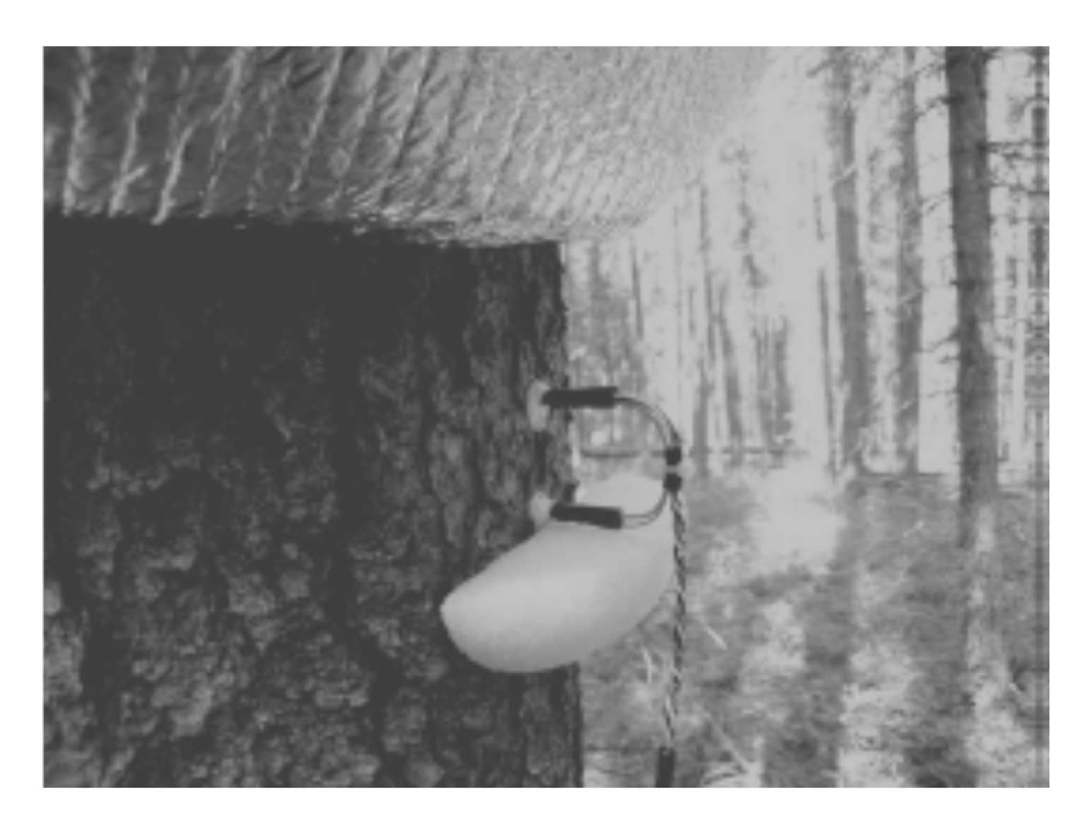
Sap flow in a single tree was measured using the heat dissipation technique [51]. At each plot, a group of four trees (for each species inside the plot) were set up with thermal dissipation probes (TDP-30, Dinamax, Inc., Houston, TX, USA) for periods of 48 h. The thermal dissipation probes (TDP’s) were installed in the North side of the trees and covered with a special insulating material (Figure 2) to avoid direct solar incidence and overheating of the sensors that might alter the logger readings. At the same time, a set of soil moisture sensors (six sensors) was placed in the soil (below the litter) to observe the changes in soil moisture content and to later compare with the trees’ water uptake. The soil moisture values are also used in the empirical calculation of . After 48 h, another group of four trees was set up with the TDP’s and soil moisture sensors. This task was performed at least four times within each plot. We were interested in capturing the sap flow patterns of trees with different diameters (i.e., interspecific heterogeneity); therefore, the trees selected for measuring daily sap mass flow were chosen in order to cover the range of trees’ outside bark diameter at breast height () in each plot (i.e., the largest, the smallest, the mean, and other intermediate values of each species found inside the plot).
Sap mass flow measurements were corrected by applying the original calibration presented by Granier [52], and presented here in Appendix A. The canopy transpiration estimates were computed after sap mass flow data were corrected for radial patterns of sap flow. Trembling aspen individuals were excluded from the radial correction, since it had been proven that diffuse-porous tree radial sap flow does not vary significantly [18,53,54]. The method to compute canopy transpiration from sap mass flow data is detailed in Section 2.2.
In order to validate the scaled transpiration values, the actual forest evapotranspiration () and plant actual transpiration () were estimated for both sites. The former estimate was computed using the Penman–Monteith equation, while the latter was computed using a modified version of the Penman–Monteith equation [47]. The mathematical theory behind the three models’ computations is detailed in Section 2.3 and Section 2.4.
The meteorological data required to compute and were collected using a HOBO meteorological station (Onset Computer Corporation, Bourne, MA, USA), which was set up in a 25 m radius clearing located inside the Barrier Lake forestry trails nearby. The installed sensors measured temperature, relative humidity, dew point, rainfall, atmospheric pressure, wind speed, gust speed, wind direction, solar radiation, and photosynthetically active radiation. The sensors were placed at height of about 3 metres above the ground level. All the variable data were collected every minute.
The sap flow values were assessed by observing the order of magnitude and their agreement between some meteorological variables and the sap flow trends. It was expected that sap flow rates would be greater in sunny, calm days than in rainy, cold, cloudy days, with a plateau at night. There are periods of the day when sap flow decreases to avoid desiccation, and some other periods in which it is known that all trees reach their maximum sap flow rates.
2.4. Scaling Actual Canopy Transpiration
2.4.1. Radial Patterns of Sap Flow
The acropetal sap transport rate has a radial gradient that decreases from the outermost part of the sapwood towards the pith. Since there is enough evidence of the significance of the sap flow radial gradient while scaling up sap flux density from a single point to the entire tree [17,18,24,55,56] a sap flow radial profile function developed by [57] was used to calculate the sap flow velocity along the entire sapwood depth of each tree. The radial profile function accounts for the fractional changes in sap flow as a function of the maximum sap flow rate, the sapwood depth at which this rate occurs, the total sapwood depth and the rate at which the sap flow velocity decreases from the outer to the inner sapwood:
where is the sap flow rate index (expressed as a fraction), is the maximum sap flow rate (equal to 1.0) occurring at the sapwood depth, and is the rate at which the sap flow radially decreases towards the pith’s trunk. In order to calculate sap flow velocity changes instead of fractional changes, Equation (1) was modified to the following form:
where is the sap flow velocity in the first three centimeters of sapwood, and the maximum sap flow velocity is . Studies in variations of radial sap flow have found that in conifers, the maximum velocity or the largest portion of sap flow occurs in the first centimetre [17], the first 2 cm and 3 cm [58] of sapwood depth (from cambium to pith). Research outcomes [56] reported graphs showing that maximum sap flow occurs at 20% of the depth (from cambium to pith as well). It seems that the depth at which the maximum sap flow occurs is a standard pattern independent of the tree size. Based on these previous results, here it is assumed that Vₘₐₓ occurs somewhere between the first two centimeters; thus, x₀ = 2 cm. Other studies have reported that the rate of decrement in radial sap flow is about 20–24% in conifers; thus, has been assumed to equal 4 (i.e., a 25% of decrement). As V₀–₃ is known; that is, it is calculated from the field measurements, Vₘₐₓ can be estimated from Equation (2). Finally, Vₘₐₓ is used to estimate the sap flow velocity along the entire sapwood depth () at a specific time:
Note that is , the original symbol used by [53] to define sap flow velocity; thus,
where the sap flow velocity, (cm s−1), is converted into the total trunk’s mass flow, , (cm3 s−1), by scaling from the point of measurement, to the total sapwood cross-sectional area, (cm2). Values of were computed with Equation (3) at each time step (5 min) and then used to estimate each tree’s daily .
To estimate an average canopy transpiration rate, , single tree transpiration values where scaled up to the whole plot. First, a diurnal average sap flow per species was estimated, and multiplied by the total sapwood area of that species inside the plot, obtaining the total average canopy water mass flow:
and
where is the average sap flow velocity of the species obtained by the summation of the diurnal average sap flow velocity of each ith individual and divided by the total individuals of the same species whose sap flow was measured. is the average of the species total mass flow, and is the total sapwood area of the species . present in a specific plot The calculation of the average canopy water mass flow () is through the summation of each plot’s species total water mass flow:
The average sap flow within the plot is:
To estimate , the is normally divided by a unit area of ground (i.e., 1 ha). This division allows one to observe the agreement between canopy transpiration and actual forest evapotranspiration (), or actual forest transpiration (). Here, we assessed three different units of surface ground area: Plot sapwood area (), the actual leaf area (), and the effective leaf area (). Finally, values were compared with an average of and .
2.4.2. Azimuthal Sap Flow Variation
Previous work [27] where we reported that we measured sapwood depth in four different sides of the tree to account for the sapwood depth variation around the tree trunk, and therefore the azimuthal variation in sap flow. The sapwood depth was measured under the microscope, and for each tree, an average sapwood depth was computed. We consider that this is sufficient to account for azimuthal sap flow variation.
2.4.3. Water Storage Capacity Estimates
It is assumed that the water stored in the tree trunk equals the amount of water replenished at night. The assumption is based on previous research focused on the contribution of a tree trunk’s stored water to transpiration, under dry and wet conditions. Reported results show that on average, of the daily amount of water transpired by a tree, 14.8–20.0% corresponds to the trunk’s stored water [59,60,61,62]. In Trembling aspen, the water trunk provided 11.6% of the mean daily transpiration [61] and most of the time, full replenishment for the tree trunk occurs at night [60], which creates a water balance between the tree water lost during the day and the water recharged at night. In addition, it has been determined that for scaling purposes, the error associated with water storage capacity is practically null if between individuals, the sap flux variability is low [60].
2.5. Estimating Actual Forest Evapotranspiration
The Penman–Monteith equation estimates the actual evapotranspiration of vegetated surfaces by accounting for all the micrometeorological factors that influence evapotranspiration as well as the influence of the canopy conductance and aerodynamic resistance in the rates of vegetation transpiration:
where is the latent heat of actual evapotranspiration, is the slope of the saturation vapor pressure curve (kPa°C−1), is the net solar radiation, and is the soil heat flux (all these terms in units of (J m−2 s−1)). The air density is denoted by (kg m−3) and is the specific heat of air at constant pressure (i.e., 1010 Jkg−1°C−1). The term is the vapor pressure deficit () calculated by the difference between the saturation vapor pressure (, (kPa)) and the actual vapor pressure (, (kPa)). The psychrometric constant is in units of (kPa°C−1). The aerodynamic terms, and are the aerodynamic resistance to vapor and heat transfer, and the bulk canopy resistance (both expressed in sm−1). To convert the latent heat of evapotranspiration to actual evapotranspiration (), in units of mms−1 was employed. The equations used to solve the aerodynamic and energy parameters of the Penman–Monteith equation are detailed in Appendix A.
2.6. Estimating Actual Canopy Transpiration
Liu et al. [47] presented a modified version of the Penman–Monteith equation in order to estimate actual canopy transpiration at large scales. According to Liu et al. [47], a model such as Penman–Monteith should be adjusted by separately estimating the transpiration of shaded and sunlit leaves as follows (stratified model):
where and are the actual transpiration of sunlit and shaded leaves, respectively; and are the leaf area indices for sunlit and shaded leaves as well. The Penman–Monteith equation is then used by Liu et al. [47] to estimate and :
and
where and are the net solar radiation available for sunlit and shaded leaves (Jm−2s−1), respectively, and is the stomatal resistance (sm−1). The rest of the parameters and units remain the same as in Equation (9).
The boreal ecosystem productivity simulator (BEPS) provides a set of equations to calculate and (Liu et al., [47,63]). The equations compute the shortwave solar radiation for sunlit and shaded leaves as well. The net longwave solar radiation is assumed to behave equally for sunlit and shaded leaves; therefore, a single equation is used to calculate net longwave solar radiation. Thus, and are respectively given by:
and
where and are the shortwave solar radiation for sunlit and shaded leaves, respectively, and and are the net longwave solar radiation for sunlit and shaded leaves, respectively. The solution to these equations is formulated in Appendix A, and also provided by Liu et al. [47].
3. Results
Not all of the instrumented trees provided credible data and after all the sap flow data collection were checked for quality, only four Trembling aspen, five Lodgepole pine, and four White spruce trees provided credible sap flow measurements adequate for scaling up to the plot scale. In the case of the Coniferous site, eight days of sap flow measurements were used to calculate and . The Deciduous site provided four days of sap flow measurements and meteorological data. For the same dates, and were computed. Each site’s daily values were averaged and compared with the average obtained for their respective time periods.
3.1. Scaling Canopy Transpiration
The Deciduous plot’s ratio of to the plot’s basal area was 0.57, while in the Conifer site, the ratio was 0.54 for the Lodgepole pine trees and 0.38 for the White spruce trees. Thus, the Trembling aspen showed a larger sapwood area per unit basal area at the plot scale than the conifer species. That was expected since diffuse-porous trees have larger sapwood areas in order to meet their water demand (i.e., they are less efficient at transporting water). As it is shown in the following sections, the Deciduous site drew larger mass flow per plot than the Coniferous site.
Figure 3, Figure 4 and Figure 5 exemplify the diurnal sap flow patterns in Lodgepole pine, White spruce, and Trembling aspen. In each plot, the dashed line is and the solid line is . Two individuals of different DOB are presented in order to exemplify the differences in Ji due to the tree size. Notice that the Lodgepole pine Ji is somewhat tempered in comparison to .
Each tree’s sap flow pattern was analyzed in order to determine the times of initial and final daily transpiration activity. The transpiration patterns of the sampled trees showed activity starting early in the morning (around 500 and 545 h) and finishing between 1700 and 1900 h. Variations in the time at which the tree stopped transpiring and starting transpiring again were related to the meteorological changes.
The radial profile function to correct the sap flow velocity showed that the sap flow velocity values could have an underestimation of 12.5% in trees with a relatively small sapwood depth (3.5 ± 1.5 cm). The average in conifers ranged between 3.10 cm and 3.50 cm. In this particular case, if the radial profile correction could not be applied, the sap velocity will be underestimated when scaled to the entire tree. Each species, and are reported in Table 1. The Coniferous site total mass flow is the summation of the two species populating the site.
3.2. Actual Evapotranspiration Results
All the mathematical models to calculate are detailed in Appendix A. The most complex parameter to obtain is . A series of reduction functions were used, and the assumptions made provided half-hourly values that are in reasonable agreement with the values listed by [64,65,66]. The other parameter that was estimated in an uncommon way was . This was done by integrating parameters that take into account the influence of , gap fraction and emmisivity of understory and overstory. Since the determination of and was essentially based on previous reports, which at the same time are based on a few assumptions, it was necessary to observe the influence of and values on the calculation of . Thus, a sensitivity analysis of was performed by using different and values. The range of values to test and were 0.6–1.5 and 0.5–0.9, respectively. The obtained estimates of with respect to the initial differ in the range of −2.0 × 10⁻⁴ to 9.0 × 10⁻⁴ mmd−1. When and are set up as 0.6 and 0.9, respectively, estimates are practically the same as when and are set up as 1.0 and 0.5 (the values used here), respectively. The sensitivity analysis was also performed to see the impact on the average of (i.e., ) per day. The analysis showed differences among values in the range of 2.0 × 10⁻⁴ to 6.0 × 10⁻⁴. In conclusion, the assumed and values were considered adequate. Final estimates of are listed in Table 2. The values are shown per date and sorted by the type of site that was set up for sap flow measurements in the same dates.
Liu et al. [47] reported that Canadian boreal forest evapotranspiration values range between 100 and 300 mm year−1. Additionally, Liu et al. [47] estimated that a coniferous land cover could have a yearly transpiration of 123 mm with an s = 55 mm; and deciduous and mixed forests land covers were reported with yearly transpiration values of 327 mm and 244 mm, respectively. On examination of the previous results, it would seem that there is an overestimation of ; however, 2004 had a particularly wet and hot summer, that exceeded reported rainfall normals [67] by a factor of 0.75 in July and 2.27 in August. Moreover, daily maximum temperatures during the months of July and August were greater than the daily maximum values reported in Environment Canada’s Climatic Normals [68]. That is, July and August maximum temperatures varied between 24 and 29 °C, respectively, while the Climatic Normals reported maximum temperatures of 21.5 and 21.1 °C, respectively. Thus, the conditions for large evapotranspiration amounts that are greater than normal maximums could be considered reasonable for this wet and hot summer.
Variation in the Soil Field Capacity
The soils in the field plots were comprised of a sandy loam. The field capacity of a sandy loam soil varies between 0.16 and 0.22, and its wilting point is 0.073 [68]. The reported was calculated using an average value of the soil field capacity. Calculations of , , and were made using the lower and upper bounds of the soil’s .
Results showed that in days when , the function limiting was , causing to become practically null, and making reach its maximum value. In these days, there was no difference in the final since the computation of will always be zero or negative, no matter the value. Of course, in those days the factor limiting was soil moisture to the point that observed values were lower than 1 mmd−1 (e.g., days 213 and 235, Coniferous site).
When , soil moisture is not limiting at all, and other environmental factors drive . In these cases, there was no variation in the final estimate. It was noticed as well that the immediate limiting factor was , and then (e.g., days 231, Coniferous site).
Finally, if , there is variation in the estimates of . This was noticeable for just two days in the whole data set used here (days 215 and 216, set up in the Conifer site). When varied from 0.0750 to 0.0795, the changes in generated to vary between and , when was set up as 0.22 and 0.16 respectively (day 215). When varied from 0.0735 to 0.0743, the changes in caused of , either was 0.22 or 0.16, respectively (day 216). The reported values for these two days are and . In those two days, it could be said that there is a variation in the estimates between and .
3.3. Actual Canopy Transpiration Results
Appendix A details the mathematical models, and the computation of and is very similar to the one applied for computing . The main changes rely on substituting by either or and the use of instead of . Table 3 and Table 4 show the obtained transpiration estimates for shaded, sunlit leaves, and the total canopy transpiration in the Conifer and Deciduous sites, respectively. It is worth mentioning that for the Deciduous site, the estimates were based on the estimation of computed with .
Variation of the Soil Field Capacity
As in the estimates, there is variation in the estimates of if . At the Coniferous site, days 215 and 216 showed the variations at the Coniferous site. When varied from 0.0750 to 0.0795, the changes in generated to vary between and , (keeping equal to 0.22 and 0.16 respectively; day 215). When varied from 0.0735 to 0.0743, the changes in caused of , either was 0.22 or 0.16, respectively (day 216). The reported values for these two days are and . In those two days, it could be said that there is a variation in the estimates between and .
3.4. Agreement between Methods
The Coniferous site’s daily average estimates of and (Table 2 and Table 3) are practically the same (). For the Deciduous site by . Hence, both Equations (9) and (10) draw very similar estimates. Such close similarity could mean that the wet, hot summer conditions of the studied area made the evaporation component negligible. Nevertheless, this should be part of future studies that could observe the agreement between the original Penman–Monteith equation and the stratified model developed by Liu et al. [47].
The comparison between and is shown in Table 5, while Table 6 shows the comparison between and . For these comparisons, the transpiration values are expressed as the average of the [] measured in the trees inside of each plot per unit ground area. This unit ground area was estimated as the ratio of per (from now on referred to as “ as unit ground area”). Additionally, and were averaged (i.e., and ) on the same days for which was computed.
The agreement between the Coniferous and is acceptable and showed that is about 97% of the total forest evapotranspiration. The remaining of may be attributed to the other sources of forest evapotranspiration such as surface evaporation and understory transpiration. The contribution of understory evapotranspiration varies and it could be fairly large during the growing season; however, [69] listed different sources that measured understory in stands of different pinaceas, and percentages range from 6% to 60% as understory contribution to forest . Thus, it is reasonable to attribute the difference between both methods to understory . Very similar results were seen in the comparison between and where is 97% of the estimates. Although both values are quite similar, the is greater than by . The agreement is acceptable as well; however, it was expected that both values would be equal (i.e., ).
The Deciduous plot results showed a better agreement with when was set as and . In this case, is about 73% of , and about 71% of . This value can also be considered acceptable as well, since the days when the was measured, the soil moisture was not limiting, and was the driving factor. As it has been shown in other works [52], when this situation happens, the sap flow reaches a plateau and becomes quasi constant along the day. Just as when water is limiting, decreases. Thus, the remnant 28% of the may be attributed to the understory transpiration and other surfaces of evaporating water.
3.5. Leaf Area Indices as Scaling Factors
Assessing other unit areas that could be helpful in transforming sap flux density values into a canopy transpiration rate, effective leaf area () and actual leaf area () were used as unit areas as well:
where
or
where
Leaf area values are the same values as those used to create the regression model with in [25]. Results are shown in Table 7 and Table 8. As it is appreciated, and as unit ground areas describe the canopy transpiration of the Coniferous site as 48% and 67% of , respectively; and the same agreements are shown with . In the case of the Deciduous site, is described as 64% and 83% of . On the other hand, is 62% and 80% of . The as a unit area describes the Deciduous as a larger proportion of than the unit ground area when these values are based on ).
4. Discussion
The main objectives of this study involve scaling issues in transpiration: firstly, to identify those parameters influencing transpiration at different scales in order to use them as scaling parameters if adequate models can be developed [25,26,28]; and secondly (but no less important), the improvement of the final transpiration estimates at larger scales. This is a complex task since there often exists large intra- and interspecific variability that, at the same time, is controlled by biophysical characteristics. In this study, these problems were faced and addressed by using more accurate methods to estimate the scaling factors in order to avoid large uncertainty in the final estimates. The effectiveness of using more accurate methods is proven through the validation of estimates. That is, will be reasonable result if first, , or at least ; and second, will be a significant proportion of .
Each site’s shows an acceptable agreement with the computed actual forest evapotranspiration and the actual canopy transpiration—Equations (9) and (10). In the Deciduous site case, the obtained motivates one to speculate if the agreement is good enough. In this particular case there is an issue worth mentioning here (in case the reader considers the fraction to be small). The days in which the was calculated, showed large and values because was not limiting, and was driving and transpiration as well. In this case, the empirical factor was adjusted as much as possible by respecting previous reports on the influence of on . The actual of the Trembling aspen individuals could go beyond the empirical estimates, but there is no field data that could evince this and allow modification to . Moreover, BEPS results suggest that at larger scales, a deciduous forest’s transpiration is about 67% of the annual actual forest evapotranspiration [47]. Therefore, the Deciduous are considered reasonable estimates.
The three different area factors that were used to calculate actual canopy transpiration drew dissimilar results. Still, the three estimated values always met the expected agreements with and . The Coniferous site estimated by means of as a unit ground area (i.e., using ) implies that there is a significant contribution of canopy transpiration to the total of the studied sites. Moreover, the estimated . Thus, the canopy transpiration rates are in good agreement with previous works when using as the unit ground area.
However, using any leaf area as a unit area factor, it seems that canopy transpiration is underestimated (in the Coniferous site), and overestimated (in the Deciduous site) in comparison with the obtained using as unit area. The as a unit ground area that defines the Deciduous site’s as a larger fraction of (than that estimated with as unit ground area). Thus, becomes a larger proportion of than using as a unit ground area. Conversely, as a unit ground area defines the Coniferous site’s as a smaller fraction. Results suggest that as unit ground area gives adequate estimates for the Coniferous site and the gives adequate estimates for the Deciduous site. Hence, the chosen unit ground area considerably influences the estimates.
With respect to the results from Equations (9) and (10), it was expected that will be a significant proportion of (i.e., between 70% and 90%). However, the daily values of and slightly differ; and most days showed that indeed (i.e., Days 212, 215, 216, 234, 225, 226, and 228). As it was expected, is always a significant proportion of for most days (i.e., of the . There were also days when (Days 231, 232, 235, and 227). These results suggest that there were humid days causing some water condensation. Indeed, in those days, the morning estimates (i.e., hourly values) are negative. Moreover, approximately half of each day drew .
If the volumetric soil moisture approximates its wilting point, there could be significant variations in (as well as ). Therefore, the influence of variations on was studied. During the days that this research was conducted, the soil was either extremely dry (below its ) or very wet (), causing just two days of transition between dryness and wetness to affect values.
Even though the authors’ methods help reduce the error carried out by scaling parameters, there is certainly opportunity to improve sap flow measurements. The choice to capture inter-specific variability, that is, changing the thermal probes after 48 h to individuals of different diameters, may have introduced uncertainty into the final data due to the short sampling time. The two summers in which sap flow data were collected were not the most favorable in terms of capturing sap flow patterns (such as those shown in Figure 4 and Figure 5). Overcast days were constantly present, and we were not able to observe expected diurnal sap flow patterns (e.g., Figure 3). Another challenge was that on several occasions, the probes had to be moved to different trees because the probes were not capturing sap flow activity, which was attributed to tree infestation that was not initially visible or obvious. Thus, the sample size and temporal replication of sap flow were reduced to only a few trees and only up to four and eight days of sap flow data for the Coniferous and Deciduous site, respectively. In addition, the calibration method used to account for radial variation was estimated, and many other authors could argue that in situ calibration methods are the most effective methods, but they also indicate that this is a rare practice [15]. The available calibration methods—using potometers—are invasive, and there are concerning factors with these calibration techniques. Among those concerns is the fact that the base of the tree is damaged by the removal of its outermost bark, which means that most likely the tree will suffer from embolism and most likely will die. Injecting pressurized water into a tree could also cause severe damage to the secondary xylem tissue, which is known to be extremely delicate and easily broken by slight changes in pressure. Amid climate change and the global biodiversity crisis, the intention with this research was to propose a scaling approach that will conserve and protect the forest trees and their environment; thus, the authors used those techniques that were the least invasive and did not require sacrifice or damage to the integrity of the trees.
5. Conclusions
The scaling approach proposed here was shown to be an appropriate way to quantify the variation of scaling factors [25,26,28] and to prove their correlation at large scales. The use of these scaling factors and the careful formulation of the scaling approach were fundamental in obtaining canopy transpiration estimates that closely agreed with the estimated actual evapotranspiration using the Penman–Monteith and the modified Penman–Monteith equations.
The canopy transpiration values calculated using the as a unit ground area factor are meaningful due to the close relationship between the total amount of leaves that fully operate during transpiration. Thus, we suggest that a deeper understanding and testing of this canopy transpiration number would be a significant contribution to the study of the efficiency of trees in water use. It is also recommended that prior characterization of the intraspecific biometrics’ variations be made in order to further develop the scaling approach. In addition, future work should focus on observing the behavior of this scaling approach at larger scales.
Many canopy transpiration studies disregard the impact that regression models have in the final estimates of transpiration. Previous research has demonstrated the constant over and underestimations of sapwood depth, sapwood area, leaf area, and leaf area index by using general assumptions, and the concerning level of error that these values carry to larger scales. However, the authors acknowledge that the sap flow data collected for this work would be further improved by increasing the temporal scale and sample size per species. Our suggested approach for capturing sap flow interspecific variability requires further study and thus, for future work, it is advised to measure sap flow simultaneously on a series of trees with different diameters.
Supplementary Materials
The following are available online at www.mdpi.com/xxx/s1.
Author Contributions
Conceptualization, M.R.Q.-P. and C.V.; methodology, M.R.Q.-P.; software, M.R.Q.-P.; validation, M.R.Q.-P.; formal analysis, M.R.Q.-P.; investigation, M.R.Q.-P.; data curation, M.R.Q.-P.; writing—original draft preparation, M.R.Q.-P.; writing—review and editing, M.R.Q.-P. and C.V.; supervision, C.V.; funding acquisition, M.R.Q.-P. and C.V. All authors have read and agreed to the published version of the manuscript.
Funding
This research was funded by the Alberta Ingenuity Fund, NSERC, Consejo Nacional de Ciencia y Tecnología, México, and Universidad Autónoma Metropolitana-Iztapalapa, México.
Acknowledgments
Thanks are due to the Biogeoscience Institute of the University of Calgary, Alberta. We would also like to thank the anonymous reviewers for their insightful comments.
Conflicts of Interest
The authors declare no conflict of interest.
Appendix A. Computing Actual Evapotranspiration and Canopy Transpiration
Appendix A.1. Actual Evapotranspiration
Since the direct estimation of transpiration is complex, it is more common to estimate evapotranspiration () of forested areas as a close estimate of transpiration. For dense, homogenous vegetated areas, transpiration is usually considered the largest portion of total evapotranspiration in forested areas. In Canada, it is estimated that forest transpiration has a large proportion of the total varying between 45% and 67% of total ), while the rest of the water lost is through soil evaporation or evaporation of water on surfaces (e.g., leaves and trunks) and sublimation [47]. These statements are reinforced with detailed studies of in the boreal forest that demonstrate the large activity and amounts of energy and mass fluxes [70].
In this study, the Penman–Monteith equation [71] is used to estimate the actual evapotranspiration of the vegetated areas under study. These evapotranspiration estimates will be used to validate the daily transpiration rate estimates at the plot scale. The Penman–Monteith equation estimates the actual evapotranspiration of vegetated surfaces by accounting for all the micrometeorological factors that influence evapotranspiration as well as the influence of the canopy conductance and aerodynamic resistance in the rates of vegetation transpiration:
where is the latent heat of evapotranspiration is the slope of the saturation vapor pressure curve (C), is the latent heat of actual evapotranspiration (), is the net solar radiation, and is the soil heat flux (all these terms in units of ). The air density, is in (); is the specific heat of air at constant pressure (i.e., C). The term is the vapor pressure deficit () calculated by the difference between the saturation vapor pressure (, )) and the actual vapor pressure (, )). The psychrometric constant, , is in units of (C). The aerodynamic terms, and are the aerodynamic resistance to vapor and heat transfer, and the bulk canopy resistance (both expressed in ). The following paragraphs explain in detail the calculation of each Penman–Monteith equation’s parameter. To convert the latent heat of evapotranspiration to actual evapotranspiration (), use in units of .
Appendix A.1.1. Aerodynamic Parameters
To calculate the term in the Penman–Monteith equation, the saturation vapor pressure was initially calculated using two different equations:
and
In both equations, is the air temperature (°C, field weather station measurements). The first equation is the resultant of a Chebyshev fitting procedure used by [72]. The polynomial coefficients (i.e., to ) are reported in Lowe’s paper [72] and is calculated in units. The latter equation calculates in was derived by [73] and its estimates are considered of high reliability [64]. The average difference between values calculated with both equations was of . Thus, for further estimations, Equation (A3) is applied. The actual vapor pressure is calculated using the estimated and the relative humidity (, (%)) that was measured in the field [74]:
The air density, , can be derived from [64]:
where is the daily mean atmospheric pressure calculated with the field measurements (barometer, units of ), is the specific gas constant (). is the virtual temperature in degrees Kelvin, calculated as [64]:
where and are taken as the daily average of and respectively. A sensitivity analysis was performed to observe how values affect or the evapotranspiration estimates. There were no significant changes in the values. Thus, was used in the equation. This analysis was performed since [64] did not specify if an average temperature or temperature at each hourly time-step value should be used.
The psychrometric constant can be expressed as [75]:
where is given in units of C, is entered as , P is in . The water vapor ratio molecular weight () is a constant value equal to , and is calculated using the following equation [64]:
where is given in units of (i.e., multiply by 1000 to match units of ).
The slope of the saturation vapor pressure curve () is derived from the following equation:
The aerodynamic resistance to vapor and heat flux, , is estimated with the following equation [64,76]:
where is von Karman’s constant (0.40), is the height () at which the wind speed () has been recorded ( in this particular case), is the zero-plane displacement () that is assumed as 67% of the canopy height (i.e., ) for vegetation with . Here, the average canopy height is , which is the same height used in previous estimations. The parameters and are the roughness lengths for the momentum and heat transfer, respectively. Allen et al. [64] suggested applying . In this study, the fact that varies with cover has been taken into account; thus, is calculated differently for the Deciduous and the Coniferous sites. For the Deciduous sites, whose vegetation is considered dense and homogeneous, the equation suggested by [76] is applied:
For the Coniferous sites, the equation suggested by [64] is applied:
where is an empirical factor that is independent of vegetation height [77]. Based on their calculated values of and for conifers, [77] determined . Table 1 lists the constant terms of the aerodynamic resistance equation. The ratio calculated for Coniferous sites concurs with the mean value reported by [64] for this ratio. The Deciduous’ sites value is between the range of values listed for deciduous trees by [64].

Table A1.
Steady parameters in the calculation of the aerodynamic resistance to heat and vapor transfer, . All parameters are reported in meters, with exception of , which is unitless.
Table A1.
Steady parameters in the calculation of the aerodynamic resistance to heat and vapor transfer, . All parameters are reported in meters, with exception of , which is unitless.
| Parameter | Coniferous Sites | Deciduous Sites |
|---|---|---|
| 15 | 15 | |
| 0.22 | 0.37 | |
| 10.05 | 10.05 | |
| 1.089 | 1.82 | |
| 0.1089 | 0.1821 |
The canopy resistance is more complicated to estimate since it varies along the day and it is a function of several atmospheric parameters [78]:
This equation implies that the canopy conductance () is a function of the environmental parameters: , (), (), (°C), and volumetric soil moisture (, in ). The parameter that reaches its minimum at a specific time (), drives the canopy conductance. The lower the value of the environmental parameter reduction function, the lower the value of , therefore the higher the . Each parameter is represented by a reduction function that computes the value of the function between zero and one (i.e., ). Different authors have developed and calibrated reduction functions for calculating each one of the parameters in Equation (A13). Allen et al. [64] suggested that these equations can be replaced in the function above. Here, a set of equations was chosen and presented below. Most of the equations and empirical factors are taken from [79]; otherwise, the author is cited. Stewart [79] developed and calibrated these functions for Scots pine. This is the closest species to the species studied in this work with reported functions. In the case of the Deciduous site, the empirical factors were adjusted according to the response of or to the environmental parameters. This task was performed based on previous results and results that were obtained in this study.
The is the reciprocal of the minimum canopy or surface resistance (). Typical values reported for coniferous forests range from to [64]. Here, an average value of the reported ranges was taken for the Coniferous site (i.e., ). Ref. [80] reported maximum values of canopy conductance for Trembling aspen () and it is the one applied here for the Deciduous site. To compute :
where is the maximum LAI Along the year. Since data collection occurred during the peak of the summer (July and August), it is assumed that for both the Coniferous and the Deciduous sites. The is calculated with
where is in and is an empirical factor that was set up as .
The VPD function is established based on the two following equations:
and
with . The is called the “threshold vapor pressure deficit” and is set up as for the Coniferous site. For the Deciduous site, [52] reported the sap flow trend of four hardwood species in relation to . One of the species studied is from the genus Populus. For that result, it was reported that the Populus sap flow did not significantly vary when was greater than , unless the soil moisture content was limiting. The results presented by [52] perfectly concur with our study results. Thus, the threshold for the Deciduous site was assumed as . Since a factor was not found in the literature, its value was determined by using previously reported trends of versus . Thus, the value was assumed as initially. This decision was somehow conservative and based on the fact that deciduous reported values have reached [64]. Therefore, was set up to make the reciprocal of to quasi match to when is greater than and becomes the driving environmental parameter of . Using graphs by [80] of half-hourly changes in and , it was observed that can change from to as reaches values greater than . In this case, a second run for was performed assuming , to make when . Values of obtained with both parameters are presented here.
For calculating , a maximum and a minimum temperature ( and , in °C) is required that constrain the stomas process, plus another empirical factor, (called the “optimum conductance temperature”):
where
and is °C for the Coniferous site. In the case of the Deciduous site, reported half-hour Trembling aspen and temperature values [80] were used to estimate the optimum conductance temperature for Trembling aspen . An average optimum temperature of °C was obtained.
Finally, to estimate the , a function reported by [64], which is a slightly modified version of the one suggested by [79], was used:
where ( is the empirical factor used to calculate ; and is the fraction available for transpiration, also called the “effective fraction of available soil moisture” [64]:
where is the volumetric soil moisture (field measurements, ), is the soil wilting point and is the soil field capacity. The values of and are obtained based on the soil texture. Direct studies of the soil type and texture in the area of Kananaskis [81,82,83,84] were used to define the soil texture in the Coniferous and Deciduous sites. The soil texture, generally defined as fine sandy loam (for both areas), drew a soil field capacity ranging between 0.16 and 0.22, while the soil wilting point was estimated as 0.07 (all values in volumetric fraction).
Appendix A.1.2. Energy Parameters
The soil heat flux is calculated using a “universal relationship” developed by [85]:
has the units of . The net solar radiation is derived from the following equation [64]:
where is the shortwave solar radiation (measured in the field with a pyranometer), is the net outgoing longwave solar radiation, and is the surface’s albedo value. The term helps to calculate the fraction of incident net shortwave solar radiation that is absorbed by a specific surface. For coniferous forests, mean values are in the range of 0.09–0.15 [66,76], and deciduous forests are in the range of 0.15–0.25 [76]. Monthly albedo values for mid-latitude forests are of 0.14 during the months of July and August [86,87,88]. The net longwave solar radiation is calculated based on the emissivity values of four different surfaces and the air temperature, [47]:
where is the Stefan–Boltzmann constant (), is the air temperature (units of K). and are the Leaf Area indices of the overstory and understory respectively; and are the clumping indices of the overstory and understory; and are estimations of the transmission of diffuse radiant energy through the understory and overstory. The emissivity of the overstory, the ground, the understory, and the atmosphere are respectively represented by , , , and . Emissivity values for the first three surfaces are assigned from [47,89] as 0.98, 0.95 and 0.98, respectively. These emissivity values concur with values reported by [64]. Emissivity from the atmosphere is calculated with the following equation [76]:
where is in [] and is in degrees Kelvin. The transmission of diffuse radiant energy through the understory and overstory is given by the following two equations that were derived by [47]:
was measured for every coniferous and deciduous site (i.e., ); is more complex to measure directly and it was derived from previous reports of understory NDVI and values. Buerman et al. [90] used the reflectance values to estimate the understory NDVI and calculate indices based on understory NDVI- scatterplots developed by [91]. The values reported by [90] range between 0.6 and 1.0 (being the largest values for Black spruce and the smallest for Jack Pine). Conifers understory NDVI (NDVIu) values reported by [90] were compared with the studied Coniferous sites NDVIu calculated from the understory spectral reflectance that was recorded in the 2003 field campaign at two Coniferous and two Deciduous sites [92]. For both Coniferous and Deciduous sites, the average NDVIu is 0.8, which is 0.3 larger than the values reported by [90] in 2002 (their NDVIu range is 0.35–0.50). Using information reported by [91], ref. [90] established that an NDVIu of 0.5 corresponded to an of 1.0. On the other hand, ref. [92] established a standard value of 0.5 for broadleaf and needle-leaf forests.
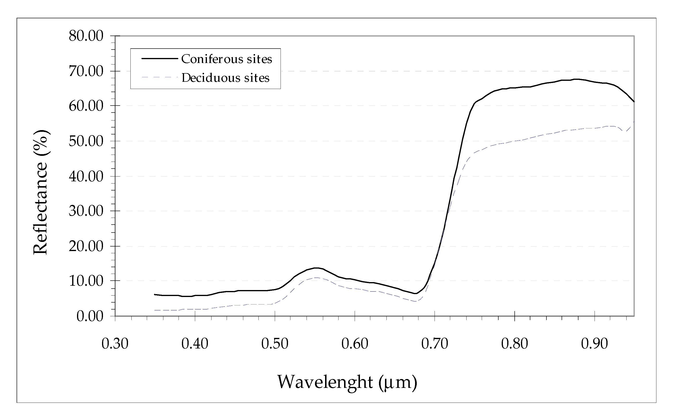
Therefore, based on these previous results, for the Coniferous sites in Kananaskis is assumed 1.0, and for Deciduous sites, 0.6. The latter value is also in the range reported by [69] for deciduous stands in a boreal forest. Figure A1 is the typical understory spectral response at a Coniferous and a Deciduous site in Kananaskis Field Station. It is convenient to stress the fact that these values are approximate; however, the main objective is to acknowledge the importance of understory in the overall evapotranspiration estimates. Thus, as [47] thought, it is convenient to somehow include the understory evapotranspiration based on assumptions about its .
Figure A1.
Typical understory spectral reflectance in Kananaskis Field Station study sites during the summer of 2003.
Figure A1.
Typical understory spectral reflectance in Kananaskis Field Station study sites during the summer of 2003.

The understory clumping index , was derived by modifying the former Chen’s equation:
where in vascular vegetation [93]. Thus, for understory vegetation does not have to be partitioned into fractions that account for the shoot effect. At the same time, the value is zero since there is no fraction of wood to account for in the understory vegetation present at the study sites. Thus,
As is known, can be approximated as 50% of as suggested by [94] for grasses (the closest that can be found to a forest understory). Hence,
Appendix A.2. Potential Evapotranspiration
The potential evapotranspiration results are provided in the
Supplementary Material section for the reader to compare the great disparity between potential evapotranspiration and actual evapotranspiration estimated with the Penman–Monteith equation. The Penman combination equation estimates the potential evapotranspiration, or also, the free water evaporation. Potential rates of evapotranspiration assume that the water is never a limiting factor, the plant completely shades the ground (thus, there is no soil evaporation) and it has the optimal environmental conditions to transpire at its maximum rate (there is no canopy resistance). Two versions of the Penman–Monteith equation are used here to estimate the Potential Evapotranspiration (), the combination equation for free water evaporation [95,96], and the Penman–Monteith equation that includes the aerodynamic parameter but sets [97]. The former equation is computed in the following form:
where is the water density in units of , and is the wind speed at height. Wind speed measured at height was scaled down to using the aerodynamic function [98]:
where is the wind speed to be estimated at height and is the wind speed at the reference height (in this case, ). Wind differences of were registered between the two heights. The rest of the parameters were already defined. The parameter is not included in the original equation; however, it was decided to slightly modify the method and include . Equation (A31) gives in units of . The second one is Equation (A1), making , and is given in :
The obtained and daily values were averaged along the eight days (for the Coniferous site) and the four days (for the Deciduous site) and compared with the average value obtained for their respective period of time.
Appendix A.3. Canopy Transpiration Using Modified Penman–Monteith Equation
Liu et al. [47] used a slightly modified version of the Penman–Monteith equation in order to estimate actual canopy transpiration at large scales. According to [47], a model such as Penman–Monteith should be adjusted by separately estimating the transpiration of shaded and sunlit leaves as follows (stratified model):
where and are the actual transpiration of sunlit and shaded leaves respectively; and are the leaf area indexes for sunlit and shaded leaves as well. The Penman–Monteith equation is then used by [47] to estimate and :
and
where and are the net solar radiation available for sunlit and shaded leaves in , and is the stomatal resistance in units of . The rest of the parameters and units remain the same as in Equation (A1). The boreal ecosystem productivity simulator (BEPS) sets up a set of equations to calculate and [47,63]. The equations compute the shortwave solar radiation for sunlit and shaded leaves as well. The net longwave solar radiation is assumed to behave equally for sunlit and shaded leaves; therefore, a single equation is used to calculate net longwave solar radiation. Thus, and are respectively given by
and
where and are the shortwave solar radiation for sunlit and shaded leaves, respectively, and and are the net longwave solar radiation for sunlit and shaded leaves, respectively. The shortwave solar radiation terms are calculated by the following equations:
where is the leaf scattering coefficient (constant that equals 0.25); is the mean leaf–sun angle, which is taken as [47]; is the solar zenith angle; and is the direct shortwave solar radiation. is calculated with
where is the diffuse shortwave solar radiation; is the diffuse shortwave solar radiation under the overstory; and accounts for the multiple scattering of direct radiation, which is calculated by
is a function of and :
and can be estimated using the following cases:
where is calculated as a function of the solar constant (), and :
and finally, can be calculated as a function of , , , and the angle for diffuse radiation ():
where is calculated using Equation (A27). The is of course the clumping index of the overstory, which is taken as 0.83 and 0.64 for the Coniferous and Deciduous site respectively (values obtained in situ with the TRAC optical device). As mentioned, the net longwave radiation terms are considered to behave the same for sunlit and shaded leaves. Thus, , and their value is calculated by
and Equation (A24) calculates . As it is noticed, Equations (A35) and (A36) include the term instead of . The stomatal resistance is calculated based on the values obtained with the set of reduction functions that resolve (Equations (13)–(21)) and with the :
Allen et al. [94] reported the previous equation using a value which is standardized for crops and relatively tall grasses (i.e., ). Here, the equation is modified to make it applicable to overstory. In addition, it is considered that shaded and sunlit leaves have similar stomatal resistances responses.
Appendix A.4. Calibration of Tree Sap Flow Measurements with TDPs
In theory, when the sap flow is constant, [52] assumed that the sap’s velocity is
where is the maximum temperature difference given when the sap flow is null (i.e., ), is the difference in temperature between the two probes at a specific time. The ratio between the temperature differences becomes the calibrated constant (flux index) in Granier’s 1985 technique [52]. With a sample size of 53 trees of three different species and diameters, [52] determined that the flux index has an exponential relationship with the velocity of sap flow:
with a , and units of are . is expressed in the same way as sap flux density; that is, flow rate of sap volume per unit of sapwood area (i.e., ). Substituting into Equation (A48) by Equation (A49), and considering the term independent of the experimentation the sap flow velocity is estimated by
where is in units of . Granier [52] validated his results with the Penman equation outcomes, finding a good agreement between both set of results (of course, Penman potential evapotranspiration estimates were greater than the ones obtained with the Granier method). The studied species were Douglas fir (Pseudotsuga menziesii), European black pine (Pinus nigra), and Oak tree (Quercus pedunculata). In this study, radial flow is correct and azimuthal sap flow variation was corrected by measuring sapwood depth in four sides of the tree to obtain an average sapwood depth and capture sapwood depth variation around the tree trunk [25,26,28].
References
- Jia, G.E.; Shevliakova, P.; Artaxo, N.; De Noblet-Ducoudré, R.; Houghton, J.; House, K.; Kitajima, C.; Lennard, A.; Popp, A.; Sirin, R.; et al. Land–climate interactions. In Climate Change and Land: An IPCC Special Report on Climate Change, Desertification, Land Degradation, Sustainable Land Management, Food Security, and Greenhouse Gas Fluxes in Terrestrial Ecosystems; IPCC—Intergovernmental Panel on Climate Change: Geneva, Switzerland, 2019. [Google Scholar]
- Bates, B.C.; Kundzewicz, Z.W.; Wu, S.; Palutikof, J.P. Climate Change and Water. In Technical Paper of the Intergovernmental Panel on Climate Change; IPCC Secretariat: Geneva, Switzerland, 2008; 210p, Available online: https://www.ipcc.ch/publication/climate-change-and-water-2/ (accessed on 2 September 2020).
- Qu, Y.; Zhuang, Q. Evapotranspiration in North America: Implications for water resources in a changing climate. Mitig. Adapt Strag. Glob. 2019, 2019, 1–16. [Google Scholar] [CrossRef]
- Zhang, K.; Kimball, J.S.; Ramakrishna, R.N.; Running, S.W.; Hong, Y.; Gourley, J.J.; Yu, Z. Vegetation Greening and Climate Change Promote Multidecal Rises of Global Land Evapotranspiration. Sci. Rep. 2015, 10, 2–9. [Google Scholar] [CrossRef]
- Boulanger, Y.; Taylor, A.R.; Price, D.T.; Cyr, D.; McGarrigle, E.; Rammer, W.; Sainte-Marie, G.; Beaudoin, A.; Guindon, L.; Mansuy, N. Climate change impacts on forest landscapes along the Canadian southern boreal forest transition zone. Land. Ecol. 2017, 32, 1415–1431. [Google Scholar] [CrossRef]
- Drobyshev, I.; Gewehr, S.; Berninger, F.; Bergeron, Y. Species specific growth responses of black spruce and trembling aspen may enhance resilience of boreal forest to climate change. J. Ecol. 2013, 101, 231–242. [Google Scholar] [CrossRef] [Green Version]
- Allen, C.D.; Breshears, D.D.; Mcdowell, N.G. On underestimation of global vulnerability to tree mortality and forest die-off from hotter drought in the Anthropocene. Ecosphere 2015, 6, 1–55. [Google Scholar] [CrossRef]
- Kingston, D.G.; Todd, M.C.; Taylor, R.G.; Thompson, J.R.; Arnell, N.W. Uncertainty in the estimation of potential evapotranspiration under climate change. Geophys. Res. Lett. 2009, 36, L20403. [Google Scholar] [CrossRef] [Green Version]
- Lijie, S.; Puyu, F.; Wang, B.; Liub, D.L.; Cleverly, J.; Fang, Q.; Yud, Q. Projecting potential evapotranspiration change and quantifying its uncertainty under future climate scenarios: A case study in southeastern Australia. J. Hydrol. 2020, 584, 1–14. [Google Scholar] [CrossRef]
- Mobilia, M.; Schmidt, M.; Longobardi, A. Modelling Actual Evapotranspiration Seasonal Variability by Meteorological Data-Based Models. Hydrology 2020, 3, 50. [Google Scholar] [CrossRef]
- Shwetha, H.R.; Kumar, D.N. Estimation of Daily Actual Evapotranspiration Using Vegetation Coefficient Method for Clear and Cloudy Sky Conditions. IEEE J. Sel. Top. Appl. Earth Obs. Remote Sens. 2020, 3, 2385–2395. [Google Scholar] [CrossRef]
- Lu, P.; Urban, L.; Zhao, P. Granier’s Thermal Dissipation Probe Method for Measuring Sap Flow in Trees: Theory and Practice. Acta Botanica Sinica 2004, 466, 631–646. [Google Scholar]
- Flo, V.; Martinez-Vilalta, J.; Sttepe, K.; Schuldt, B.; Poyatos, R. A Synthesis of Bias and Uncertainty in sap flow methods. Agric. For. Meteorol. 2019, 271, 362–374. [Google Scholar] [CrossRef]
- Peters, R.L.; Fonti, P.; Frank, D.C.; Poyatos, R.; Pappas, C.; Kahmen, A.; Carraro, V.; Prendin, A.L.; Schneider, L.; Baltzer, J.L.; et al. Quantification of Uncertainties in conifer sap flow measured with the thermal dissipation method. New Phytol. 2018, 219, 1283–1299. [Google Scholar] [CrossRef] [PubMed] [Green Version]
- Pasqualotto, G.; Carraro, V.; Menardi, R.; Anfodillo, T. Calibration of Granier Type (TDP) Sap Flow Probes by a High Precision Electronic Potometer. Sensors 2019, 19, 2419. [Google Scholar] [CrossRef] [PubMed] [Green Version]
- Nhean, S.; Ayutthaya, S.I.N.; Rocheteau, A.; Do, F.C. Multi-species test and calibration of an improved transient thermal dissipation system of sap flow measurement with a single probe. Tree Physiol. 2019, 39, 106161070. [Google Scholar] [CrossRef] [PubMed]
- Granier, A.; Anfondillo, T.; Sabatti, M.; Cochard, H.; Dreyer, E.; Tomasi, M.; Valentini, R.; Bréda, N. Axial and radial water flow in the trunks of oak trees: A quantitative and qualitative analysis. Tree Physiol. 1994, 14, 1383–1396. [Google Scholar] [CrossRef] [Green Version]
- Phillips, N.; Oren, R.; Zimmerman, R. Radial patterns of xylem sap flow in non-diffuse and ring-porous tree species. Plant Cell Environ. 1996, 19, 983–990. [Google Scholar] [CrossRef]
- Nadezhdina, N.; Cěrmák, J.; Ceulemans, R. Radial patterns of sap flow in woody stems of dominant and understory species: Scaling errors associated with positioning of sensors. Tree Physiol. 2002, 22, 907–918. [Google Scholar] [CrossRef] [Green Version]
- Ford, C.R.; Hubbard, R.M.; Kloeppel, B.D.; Vose, J.M. A comparison of sap-flux based evapotranspiration estimates with basin-scale water balance. Agric. For. Meteorol. 2007, 145, 176–185. [Google Scholar] [CrossRef]
- Zhao, H.; Yang, S.; Guo, X.; Peng, C.; Gu, X.; Deng, C.; Chen, L. Anatomical explanations for fcute depressions in radial pattern of axial sap flow in two diffuse-porous mangrove species: Implications for water use. Tree Physiol. 2020, 38, 277–287. [Google Scholar]
- Baiamonte, G.; Motisi, A. Analytical Approach Extending the Granier method to radial sap flow patterns. Agric. Water Manag. 2020, 231, 105988. [Google Scholar] [CrossRef]
- Fan, J.; Guyot, A.; Ostergaard, K.T.; Lokington, D.A. Effects of early wood and latewood on sap flux density-based transpiration estimates in conifers. Agric. For. Meteorol. 2018, 15, 264–274. [Google Scholar] [CrossRef]
- Cermak, J.; Nadezhdina, N. Sapwood as the scaling parameter defining according to xylem water content or radial pattern of sap flow? Ann. Sci. For. 1998, 55, 509–521. [Google Scholar] [CrossRef] [Green Version]
- Quiñonez-Piñón, M.R.; Valeo, C. Assessing the Translucence and Color-Change Methods for Estimating Sapwood Depth in Three Boreal Species. Forests 2018, 9, 686. [Google Scholar] [CrossRef] [Green Version]
- Quiñonez-Piñón, M.R.; Valeo, C. Allometry of Sapwood Depth in Five Boreal Species. Forests 2017, 8, 457. [Google Scholar] [CrossRef] [Green Version]
- Wang, H.; Gaun, H.; Simmons, C.T.; Lockington, D.A. Quantifying sapwood width for three Australian native species using electrical resistivity tomography. Ecohydrology 2016, 9, 83–92. [Google Scholar] [CrossRef]
- Quiñonez-Piñón, M.R.; Valeo, C. Scaling Approach for Estimating Stand Sapwood Area from Leaf Area Index in Five Boreal species. Forests 2019, 10, 829. [Google Scholar] [CrossRef]
- Aparecido, L.M.T.; dos Santos, J.; Higuchi, N.; Kunert, N. Relevance of wood anatomy and size of Amazonian trees in the determination and allometry of sapwood area. Acta Amazonica 2019, 49, 1–10. [Google Scholar] [CrossRef]
- Lubczynski, M.W.; Chavarro-Rincon, D.C.; Rossiter, D.G. Conductive sapwood area prediction from stem and canopy areas—Allometric equations of Kalahari trees, Botswana. Ecohydrology 2017, 10, e1856. [Google Scholar] [CrossRef]
- Forrester, D.I.; Benneter, A.; Bouriaud, O.; Bauhus, J. Diversity and competition influence tree allometric relationships—Developing functions for mixed-species forests. J. Ecol. 2017, 105, 761–774. [Google Scholar] [CrossRef] [Green Version]
- Mitra, B.; Papuga, S.A.; Alexander, M.R.; Swetnam, T.L.; Abramson, N. Allometric relationships between primary size measures and sapwood area for six common tree species in snow-dependent ecosystems in the Southwest United States. J. For. Res. 2019. [Google Scholar] [CrossRef] [Green Version]
- Renner, M.; Hassler, S.K.; Blume, T.; Weiler, M.; Hildenbrandt, A.; Guderle, M.; Schymanski, S.J.; Kleidon, A. Dominant controls of Transpiration along a Hillslope transect inferred from ecohydrological measurements and thermodynamic limits. Hydrol. Earth Syst. Sci. 2016, 20. [Google Scholar] [CrossRef] [Green Version]
- Dean, T.J.; Long, J.N. Variation in sapwood area-leaf area relations within two stands of Lodgepole pine. For. Sci. 1986, 32, 749–758. [Google Scholar]
- Dean, T.J.; Long, J.N.; Smith, F.W. Bias in leaf area-sapwood area ratios and its impact on growth analysis in Pinus contorta. Trees 1988, 2, 104–109. [Google Scholar] [CrossRef]
- Granier, A.; Huc, R.; Barigah, S.T. Transpiration of natural rain forest and its dependence on climatic factors. Agric. For. Meteorol. 1996, 78, 19–29. [Google Scholar] [CrossRef]
- Ewers, B.E.; Mackay, D.S.; Gower, S.T.; Ahl, D.E.; Burrows, S.N.; Samanta, S.S. Tree species effects on stand transpiration in northern Wisconsin. Water Resour. Res. 2002, 38, 1103. [Google Scholar] [CrossRef]
- Kumagai, T.; Nagasawaa, H.; Mabuchia, T.; Ohsakia, S.; Kubotaa, K.; Kogia, K.; Utsumia, Y.; Kogaa, S.; Otsuki, K. Sources of error in estimating stand transpiration using allometric relationships between stem diameter and sapwood area for Criptomeria japonica and Chamaecyparis obtuse. For. Ecol. Manag. 2005, 206, 191–195. [Google Scholar] [CrossRef]
- Denny, C.; Nielsen, S. Spatial Heterogeneity of the Forest Canopy Scales with the Heterogeneity of an Understory Shrub Based on Fractal Analysis. Forests 2017, 8, 146. [Google Scholar] [CrossRef] [Green Version]
- Montesano, P.M.; Niegh, C.S.R.; Wagner, W.; Wooten, M.; Cook, B.D. Boreal Canopy Surfaces from spaceborne stereogrammetry. Remote Sens. Environ. 2019, 225, 148–159. [Google Scholar] [CrossRef]
- Saito, K.; Iwahana, G.; Ikawa, H.; Nagano, H.; Busey, R.C. Links between annual surface temperature variation and land cover heterogeneity for a boreal forest as characterized by continuous, fibre-optic DTS monitoring. Geosci. Instrum. Methods Data Syst. 2018, 7, 223–234. [Google Scholar] [CrossRef]
- Molina, E.; Valeria, O.; De Grandpre, L. Twenty-Eight Years of Changes in Landscape Heterogeneity of Mixedwood Boreal Forest Under Management in Quebec, Canada. Can. J. Remote Sens. 2018, 44, 26–39. [Google Scholar] [CrossRef]
- Legendre, P. Spatial Autocorrelation: Trouble or New Paradigm? Ecology 1993, 74, 1659–1673. [Google Scholar] [CrossRef]
- Loranty, M.M.; Ewers, B.E.; Adelman, J.D.; Kruger, E.L.; Mackay, D.S. Environmental drivers of spatial variation in whole-tree transpiration in an aspen-dominated upland-to-wetland forest gradient. Water Resour. Res. 2008, 44. [Google Scholar] [CrossRef] [Green Version]
- Tyree, M.T. Water Relations of Plants. In Eco-Hydrology, Plants and Water in Terrestrial Aquatic Environments; Bard, S.J., Wilby, R.L., Eds.; Taylor & Francis Group, Routledge Publishers: Abingdon, UK, 1999. [Google Scholar]
- Elliot-Frisk, D.L. The boreal forest. In North American Terrestrial Vegetation, 1st ed.; Barbour, M.G., Billings, W.D., Eds.; Cambridge University Press: New York, NY, USA, 1988; Chapter 2; pp. 33–62. [Google Scholar]
- Liu, J.; Chen, J.M.; Cihlar, J. Mapping evapotranspiration based on remote sensing: An application to Canada’s landmass. Water Resour. Res. 2003, 39, 1189–1203. [Google Scholar] [CrossRef]
- Peet, R.K. Forests of the Rocky Mountains. In North American Terrestrial Vegetation, 1st ed.; Barbour, M.G., Billings, W.D., Eds.; Cambridge University Press: New York, NY, USA, 1988; pp. 33–62. ISBN 978-0521261982. [Google Scholar]
- Rowe, J.S. Forest Regions of Canada; Publication No. 1300; Department of the Environment, Canadian Forestry Service: Ottawa, ON, Canada, 1972; p. 177. Available online: http://cfs.nrcan.gc.ca/pubwarehouse/pdfs/24040.pdf (accessed on 2 September 2020).
- Strong, W.L.; Leggat, K.R. Ecoregions of Alberta, 1st ed.; Report No. T/245; Alberta Forestry, Lands and Wildlife: Edmonton, AB, Canada, 1992; p. 59. [Google Scholar]
- Granier, A.; Bobay, V.; Gash, J.; Gelpe, J.; Saugier, B.; Shuttleworth, W. Vapour flux density and transpiration rate comparisons in a stand of Maritime pine (Pinus pinaster Ait.) in Les Landes forest. Agric. For. Meteorol. 1990, 51, 309–319. [Google Scholar] [CrossRef]
- Granier, A. Une nouvelle methode pour la mesure du flux de sève brute dans letronc des arbres. Ann. Sci. For. 1985, 42, 193–200. [Google Scholar] [CrossRef]
- Bovard, B.D.; Curtis, P.S.; Vogel, C.S.; Su, H.-B.; Schmid, H.P. Environmental controls on sap flow in a northern hardwood forest. Tree Physiol. 2005, 25, 31–38. [Google Scholar] [CrossRef] [PubMed] [Green Version]
- Booker, R.E. Dye-flow apparatus to measure the variation in axial xylem permeability over a stem cross section. Plant Cell Environ. 1984, 7, 623–628. [Google Scholar]
- James, S.A.; Clearwater, M.J.; Meinzer, F.C.; Goldstein, G. Heat dissipation sensors of variable length for the measurement of sap flow in trees with deep sapwood. Tree Physiol. 2002, 22, 277–283. [Google Scholar] [CrossRef] [Green Version]
- Čermák, J.; Kučera, J.; Nadezhdina, N. Sap flow measurements with some thermodynamic methods, flow integration within trees and scaling up from sample trees to entire forest stands. Trees 2004, 18, 529–546. [Google Scholar] [CrossRef]
- Ford, C.R.; McGuire, M.A.; Mitchell, R.J.; Teskey, R.O. Assessing variation in the radial profile of sap flux density in Pinus species and its effect on daily water use. Tree Physiol. 2004, 24, 241–249. [Google Scholar] [CrossRef] [Green Version]
- Mark, W.R.; Crews, D.L. Heat-Pulse velocity and bordered pit condition in living Engelman spruce and Lodgepole pine trees. For. Sci. 1973, 19, 291–296. [Google Scholar]
- Delzon, S.; Sartore, M.; Burlett, R.; Dewar, R.; Loustau, D. Hydraulic responses to height growth in maritime pine trees. Plant Cell Environ. 2004, 27, 1077–1087. [Google Scholar] [CrossRef]
- Loustau, D.; Berbigier, P.; Roumagnac, P.; Arruda-Pacheco, C.; David, J.S.; Ferreira, M.I.; Pereira, J.S.; Tavares, R. Transpiration of a 64-year-old maritime pine stand in Portugal. Oecologia 1996, 107, 33–42. [Google Scholar] [CrossRef] [PubMed]
- Hogg, E.; Hartog, G.D.; Neumann, H.H.; Zimmermann, R.; Hurdle, P.A.; Blanken, P.D.; Nesic, Z.; Staebler, R.M.; McDonald, K.C.; Black, T.A.; et al. A comparison of sap flow and eddy fluxes of water vapor from a boreal deciduous forest. J. Geophys. Res. Space Phys. 1997, 102, 28929–28937. [Google Scholar] [CrossRef] [Green Version]
- Goldstein, G.; Andrade, J.L.; Meinzer, F.C.; Holbrook, N.M.; Cavelier, J.; Jackson, P.; Celis, A. Stem water storage and diurnal patterns of water use in tropical forest canopy trees. Plant Cell Environ. 1998, 21, 397–406. [Google Scholar] [CrossRef]
- Liu, J. A process-based boreal ecosystem productivity simulator using remote sensing inputs. Remote Sens. Environ. 1997, 62, 158–175. [Google Scholar] [CrossRef]
- Allen, R.G.; Pruitt, W.O.; Businger, J.A.; Fritschen, L.J.; Jensen, M.E.; Quinn, F.H. Evaporation and transpiration. In Hydrology Handbook, ASCE Manuals and Reports on Engineering Practice No. 28, 2nd ed.; Heggen, R.J., Ed.; ASCE: New York, NY, USA, 1996; Chapter 4. [Google Scholar]
- Perrier, A. Land surfaces processes: Vegetation. In Land Surface Processes in Atmospheric General Circulation Model; Eagleson, P.S., Ed.; Cambridge University Press: Greenbelt, MA, USA, 1982; pp. 395–448. [Google Scholar]
- Jarvis, P.G.; James, G.B.; Landsberg, J.J. Coniferous forest. In Vegetation and the Atmosphere, 1st ed.; Monteith, J.L., Ed.; Academic Press Inc.: New York, NY, USA, 1976; Chapter 7; pp. 171–240. [Google Scholar]
- EC. Canadian Climate Normals 1971–2000, Report; Environment Canada: Ottawa, ON, Canada, 2006. Available online: https://climate.weather.gc.ca/climate_normals/index_e.html (accessed on 2 September 2020).
- Dunne, T.; Leopold, L.B. Water in Environmental Planning, 15th ed.; Freeman and Company Publishers: New York, NY, USA, 1998. [Google Scholar]
- Black, T.A.; Kelliher, F.M.; Wallace, J.S.; Stewart, J.B.; Monteith, J.L.; Jarvis, P.G. Processes controlling understorey evapotranspiration. Philos. Trans. R. Soc. Lond. Ser. B Biol. Sci. 1989, 324, 207–231. [Google Scholar]
- Baldocchi, D.D.; Vogel, C.A. Energy and CO2 flux densities above and below the temperature broad-leaved forest and a boreal pine forest. Tree Physiol. 1996, 16, 5–16. [Google Scholar] [CrossRef] [Green Version]
- Monteith, J.L. Evaporation and environment. In Proceedings during Symposia of the Society for Experimental Biology. The State and Movement of Water Living Organisms, Number XIX; Fogg, G.E., Ed.; Cambridge University Press: London, UK, 1965; pp. 205–234. [Google Scholar]
- Lowe, P.R. An approximating polynomial for the computation of saturation vapour pressure. J. Appl. Meteorol. 1977, 16, 100–103. [Google Scholar] [CrossRef] [Green Version]
- Murray, F.W. On the computation of saturation vapour pressure. J. Appl. Meteorol. 1967, 6, 203–204. [Google Scholar] [CrossRef]
- Dingman, S.L. Physical Hydrology, 2nd ed.; Prentice-Hall, Inc.: Upper Saddle River, NJ, USA, 2002. [Google Scholar]
- Smith, M. Report on the Expert Consultation on Revision of FAO Methodologies for Crop Water Requirements Report; Food and Agriculture Organization of the United Nations (FAO): Rome, Italy, 1990. [Google Scholar]
- Evaporation into the Atmosphere: Theory, History, and Applications, 1st ed.; Reidel: Dordrecht, The Netherlands, 1982.
- De Bruin, H.A.R.; Moore, C.J. Zero-plane displacement and droughness length fir tall vegetation, derived from a simple mass conservation hypothesis. Bound. Layer Meteorol. 1985, 31, 39–49. [Google Scholar] [CrossRef]
- Price, D.T.; Black, T.A. Estimation of forest transpiration and CO2 uptake using the Penman-Monteith equation and a physiological photosynthesis model. In Estimation of Aereal Evapotranspiration, Number 177 in IAHS, Red Books, Proceedings of an International Workshop Held during the XlXth General Assembly of the International Union of Geodesy and Geophysics, Vancouver, BC, Canada, 9–22 August 1987, 1st ed.; Black, T.A., Spittlehouse, D.A., Novak, M.D., Eds.; International Association of Hydrological Sciences: Wallingford, UK, 1987; pp. 213–227. [Google Scholar]
- Stewart, J.B. Modelling surface conductance of pine forest. Agric. For. Meteorol. 1988, 43, 19–35. [Google Scholar] [CrossRef]
- Blanken, P.; Black, T.A.; Yang, P.C.; Newmann, H.H.; Nesic, Z.; Staebler, R.; de Hartog, G.; Novak, M.D.; Lee, X. Energy balance and canopy conductance of a boreal aspen forest: Partitioning overstory and understory components. J. Geophys. Res. 1997, 102, 28915–28927. [Google Scholar] [CrossRef] [Green Version]
- Greenlee, G.M. Soils map of Bow Valley Provincial Park and adjacent Kananaskis area. In Soils Map; Alberta Research Council, Soils Division, Alberta Institute of Pedology: Edmonton, AB, Canada, 1973. [Google Scholar]
- Greenlee, G.M. Soil survey of Kananaskis Lakes area and intrepretation for recreational use. In Final Report M-76-1; Albeta Research Council, Soils Division, Albeta Institute of Pedology: Edmonton, AB, Canada, 1976. [Google Scholar]
- McGregor, C.A. Ecological land classification and evaluation. Kananaskis country. In Natural Resources Summary, Alberta Energy and Natural Resources; Resource Appraisal Section, Resource Evaluation Branch: Edmonton, AB, Canada, 1984. [Google Scholar]
- Archibald, J.; Klappstein, G.D.; Corns, I.G.W. Field guide to ecosites of Southwestern Alberta. In Special Report 8; Canadian Forest Service, Northwest Region, Northern Forestry Centre: Edmonton, AB, Canada, 1996. [Google Scholar]
- Choudhury, B.J. Estimating evaporation and carbon assimilation using infrared temperature data: Vistas in modeling. In Theory and Applications of Optical Remote Sensing, Remote Sensing Series, 1st ed.; Asrar, G., Ed.; John Wiley & Sons: Hoboken, NJ, USA, 1989; Chapter 17; p. 628. [Google Scholar]
- Dooge, J.C.I. Modelling the behaviour of water. In Forests, Climate, and Hydrology, 1st ed.; Reynolds, E.R.C., Thompson, F.B., Eds.; The United Nations University, Kefford Press: Singapore, 1988; Chapter 7; p. 227. [Google Scholar]
- Kondratyev, K.Y.; Korzov, V.I.; Mukhenberg, V.V.; Dyachenko, L.N. The shortwave albedo and the surface emissivity. In Land Surface Processes in Atmospheric General Circulation Models; Eagleson, P.S., Ed.; WMO/ICSO Joint Scientific Committee, Cambridge University Press: Greenbelt, MD, USA, 1982; pp. 463–514. [Google Scholar]
- Henderson-Sellers, A.; Wilson, M.F. Surface albedo data for climatic modeling. Rev. Geophys. Space Phys. 1983, 21, 1743–1778. [Google Scholar] [CrossRef]
- Chen, J.M.; Zhang, R.-H. Studies on the measurements of crop emissivity and sky temperature. Agric. For. Meteorol. 1989, 49, 23–34. [Google Scholar] [CrossRef]
- Buermann, W.; Wang, Y.; Dong, J.; Zhou, L.; Zeng, X.; Dickinson, R.E.; Potter, C.; Myneni, R.B. Analysis of a multiyear global vegetation leaf area index data set. J. Geophys. Res. Space Phys. 2002, 107. [Google Scholar] [CrossRef] [Green Version]
- Myneni, R.B.; Ramakrishna, R.; Nemani, R.; Running, S.W. Estimation of global leaf area index and absorbed par using radiative transfer models. IEEE Trans. Geosci. Remote Sens. 1997, 35, 1380–1393. [Google Scholar] [CrossRef] [Green Version]
- McAllister, D. Remote Estimation of Leaf Area Index in Forested Ecosystems. Master’s Thesis, University of Calgary, Calgary, AB, Canada, May 2005. [Google Scholar]
- Leblanc, S.G.; Chen, J.M.; Kwong, M. Tracing Radiation and Architecture of Canopies. In TRAC Manual Version 2.1.3, 1st ed.; Natural Resources Canada, Canada Centre for Remote Sensing: Ottawa, ON, Canada, 2002. [Google Scholar]
- Allen, R.G.; Jensen, M.E.; Wright, J.L.; Burman, R.D. Operation estimates of reference evapotranspiration. Agron. J. 1989, 81, 650–662. [Google Scholar] [CrossRef]
- Bladon, K.D.; Silins, U.; Landhäusser, S.M.; Lieffers, V.J. Differential transpiration by three boreal tree species in response to increased evaporative demand after variable retention harvesting. Agric. For. Meteorol. 2006, 138, 104–119. [Google Scholar] [CrossRef]
- Van Bavel, C.H.M. Potential evaporation: The combination concept and its experimental verification. Water Resour. Res. 1966, 2, 455–467. [Google Scholar] [CrossRef]
- Chang, M. Forests and vaporization. In Forest Hydrology, an Introduction to Water and Forests, 1st ed.; Chang, M., Ed.; CRC Press LLC: Boca Raton, FL, USA, 2002; Chapter 9; pp. 151–174. [Google Scholar]
- McCuen, R.H. Hydrological Analysis and Design, 3rd ed.; Prentice Hall: Upper Saddle River, NJ, USA, 1989. [Google Scholar]
Figure 1.
Sap flow measured at a single tree point, can provide actual tree sap flux estimates when the tree’s sapwood area is known or accurately estimated. Each tree species sap flux can provide accurate estimates of a plot’s actual transpiration by using reduced error allometric correlations of canopy structure parameters such as Leaf Area or Sapwood Area. The plot scale can provide estimates of ET and T comparable to estimates from Penman–Monteith (P-M) and Modified P-M method, respectively. Appendix A.4 details the calibration of tree sap flow measurements.

Figure 2.
Thermal Dissipation Probes (TDPs) installed in a boreal, coniferous tree with the isolation material (upper part of the picture) ready to cover the sensors and protect them from direct exposure to solar radiation that could affect the sensors’ temperature.
Figure 2.
Thermal Dissipation Probes (TDPs) installed in a boreal, coniferous tree with the isolation material (upper part of the picture) ready to cover the sensors and protect them from direct exposure to solar radiation that could affect the sensors’ temperature.

Figure 3.
An example of a Lodgepole pine tree diurnal sap flow. Tree’s diameter at breast height was 17 cm. Day of the year: 216, in 2004. Dashed line is and the solid line is .
Figure 3.
An example of a Lodgepole pine tree diurnal sap flow. Tree’s diameter at breast height was 17 cm. Day of the year: 216, in 2004. Dashed line is and the solid line is .

Figure 4.
An example of a White spruce tree diurnal sap flow. Tree’s diameter at breast height was 18 cm. Day of the year: 232, in 2004. Dashed line is and the solid line is .
Figure 4.
An example of a White spruce tree diurnal sap flow. Tree’s diameter at breast height was 18 cm. Day of the year: 232, in 2004. Dashed line is and the solid line is .

Figure 5.
An example of a Trembling aspen tree diurnal sap flow. Tree’s diameter at breast height was 31 cm. Day of the year: 228, in 2004. Dashed line is and the solid line is .
Figure 5.
An example of a Trembling aspen tree diurnal sap flow. Tree’s diameter at breast height was 31 cm. Day of the year: 228, in 2004. Dashed line is and the solid line is .

Table 1.
and (m3day−1) at each site (n is the number of individuals used per plot).
| Site | Tree Type | n | Days Averaged | ||
|---|---|---|---|---|---|
| Conifer-4 | Lodgepole pine | 5 | 12.64 | 8 | |
| White spruce | 4 | 2.57 | 15.21 1 | 8 | |
| Deciduous-6 | Trembling aspen | 4 | 32.44 | 32.44 | 4 |
1 Conifer-4 is the sum of of both species within the plot.
Table 2.
Penman–Monteith and estimates during the same days that sap flow was measured at each site (in 2004). is the daily average.
Table 2.
Penman–Monteith and estimates during the same days that sap flow was measured at each site (in 2004). is the daily average.
| Day of the Year | Conifer-4 | Day of the Year | Deciduous-6 |
|---|---|---|---|
| 212 | 1.50 | 225 | 4.79 |
| 213 | 0.78 | 226 | 5.82 |
| 215 | 3.01 | 227 | 3.29 |
| 216 | 1.68 | 228 | 3.27 |
| 231 | 0.90 | ||
| 232 | 0.87 | ||
| 234 | 3.63 | ||
| 235 | 0.07 | ||
| 1.56 | 4.29 |
Table 3.
Modified Penman–Monteith estimates during the same days that sap flow was measured at the Coniferous site. is the summation of and . is the average of the daily . All estimates are in mm/d.
Table 3.
Modified Penman–Monteith estimates during the same days that sap flow was measured at the Coniferous site. is the summation of and . is the average of the daily . All estimates are in mm/d.
| Day of the Year | |||
|---|---|---|---|
| 212 | 0.38 | 1.08 | 1.46 |
| 213 | 0.19 | 0.56 | 0.75 |
| 215 | 1.80 | 0.73 | 2.53 |
| 216 | 1.26 | 0.41 | 1.67 |
| 231 | 0.56 | 0.66 | 1.22 |
| 232 | 0.52 | 0.64 | 1.16 |
| 234 | 2.59 | 0.95 | 3.54 |
| 235 | 0.11 | 0.04 | |
| 1.56 |
Table 4.
Modified Penman–Monteith estimates during the same days that sap flow was measured at the Deciduous site (measured in 2004). is the summation of and . is the average of the daily . All estimates are in mm/d.
Table 4.
Modified Penman–Monteith estimates during the same days that sap flow was measured at the Deciduous site (measured in 2004). is the summation of and . is the average of the daily . All estimates are in mm/d.
| Day of the Year | |||
|---|---|---|---|
| 225 | 3.00 | 1.75 | 4.75 |
| 226 | 3.67 | 2.13 | 5.80 |
| 227 | 2.44 | 1.42 | 3.86 |
| 228 | 2.05 | 1.20 | 3.25 |
| 4.42 |
Table 5.
and at the Coniferous (8 days average) and Deciduous (4 days average) sites. was used as the unit ground area to estimate . All estimates in mm/d.
Table 5.
and at the Coniferous (8 days average) and Deciduous (4 days average) sites. was used as the unit ground area to estimate . All estimates in mm/d.
| Site | Scale | Agreement | ||
|---|---|---|---|---|
| Conifer-4 | 1.56 | 1.52 | canopy | |
| Deciduous-6 | 4.29 | 3.14 | canopy | |
| Deciduous-6 1 | 5.31 | 3.14 | canopy |
1 When .
Table 6.
and at the Coniferous (8 days average) and Deciduous (4 days average) sites. was used as the unit ground area to estimate . All estimates in mm/d.
Table 6.
and at the Coniferous (8 days average) and Deciduous (4 days average) sites. was used as the unit ground area to estimate . All estimates in mm/d.
| Site | Scale | Agreement | ||
|---|---|---|---|---|
| Conifer-4 | 1.56 | 1.52 | canopy | |
| Deciduous-6 1 | 4.42 | 3.14 | canopy |
1 When .
Table 7.
, , and site average canopy transpiration over eight days at the Coniferous site.
| Unit Area | Lodgepole Pine | White Spruce | Agreement | |
|---|---|---|---|---|
| 1.56 | 1.52 | 0.74 | ||
| 0.86 | 0.18 | 1.04 | ||
Table 8.
, , and site average canopy transpiration over four days at the Coniferous site.
| Unit Area | Agreement | |
|---|---|---|
| 2.75 | ||
| 3.55 | ||
Publisher’s Note: MDPI stays neutral with regard to jurisdictional claims in published maps and institutional affiliations. |
© 2020 by the authors. Licensee MDPI, Basel, Switzerland. This article is an open access article distributed under the terms and conditions of the Creative Commons Attribution (CC BY) license (http://creativecommons.org/licenses/by/4.0/).
Share and Cite
MDPI and ACS Style
Quiñonez-Piñón, M.R.; Valeo, C. Modelling Canopy Actual Transpiration in the Boreal Forest with Reduced Error Propagation. Atmosphere 2020, 11, 1158. https://0-doi-org.brum.beds.ac.uk/10.3390/atmos11111158
AMA Style
Quiñonez-Piñón MR, Valeo C. Modelling Canopy Actual Transpiration in the Boreal Forest with Reduced Error Propagation. Atmosphere. 2020; 11(11):1158. https://0-doi-org.brum.beds.ac.uk/10.3390/atmos11111158
Chicago/Turabian StyleQuiñonez-Piñón, M. Rebeca, and Caterina Valeo. 2020. "Modelling Canopy Actual Transpiration in the Boreal Forest with Reduced Error Propagation" Atmosphere 11, no. 11: 1158. https://0-doi-org.brum.beds.ac.uk/10.3390/atmos11111158
Note that from the first issue of 2016, this journal uses article numbers instead of page numbers. See further details here.