Measuring N2O Emissions from Multiple Sources Using a Backward Lagrangian Stochastic Model


1
Department of Agronomy, Purdue University, West Lafayette, IN 47907, USA
2
Department of Earth, Atmospheric and Planetary Sciences, Purdue University, West Lafayette, IN 47907, USA
*
Author to whom correspondence should be addressed.
Atmosphere 2020, 11(12), 1277; https://0-doi-org.brum.beds.ac.uk/10.3390/atmos11121277
Submission received: 28 September 2020
/
Revised: 21 November 2020
/
Accepted: 24 November 2020
/
Published: 26 November 2020
(This article belongs to the Special Issue Atmospheric Trace Gas Source Detection and Quantification)
Abstract
:Nitrous oxide (N2O) emissions from agricultural soil are substantially influenced by nitrogen (N) and field management practices. While routinely soil chambers have been used to measure emissions from small plots, measuring field-scale emissions with micrometeorological methods has been limited. This study implemented a backward Lagrangian stochastic (bLS) technique to simultaneously and near-continuously measure N2O emissions from four adjacent fields of approximately 1 ha each. A scanning open-path Fourier-transform infrared spectrometer (OP-FTIR), edge-of-field gas sampling and measurement, locally measured turbulence, and bLS emissions modeling were integrated to measure N2O emissions from four adjacent fields of maize production using different management in 2015. The maize N management treatments consisted of 220 kg NH3-N ha−1 applied either as one application in the fall after harvest or spring before planting or split between fall after harvest and spring before planting. The field preparation treatments evaluated were no-till (NT) and chisel plow (ChP). This study showed that the OP-FTIR plus bLS method had a minimum detection limit (MDL) of ±1.2 µg m−2 s−1 (3σ) for multi-source flux measurements. The average N2O emission of the four treatments ranged from 0.1 to 2.3 µg m−2 s−1 over the study period of 01 May to 11 June after the spring fertilizer application. The management of the full-N rate applied in the fall led to higher N2O emissions than the split-N rates applied in the fall and spring. Based on the same N application, the ChP practice tended to increase N2O emissions compared with NT. Advection of N2O from adjacent fields influenced the estimated emissions; uncertainty (1σ) in emissions was 0.5 ± 0.3 µg m−2 s−1 if the field of interest received a clean measured upwind background air, but increased to 1.1 ± 0.5 µg m−2 s−1 if all upwind sources were advecting N2O over the field of interest. Moreover, higher short-period emission rates (e.g., half-hour) were observed in this study by a factor of 1.5~7 than other micrometeorological studies measuring N2O-N loss from the N-fertilized cereal cropping system. This increment was attributed to the increase in N fertilizer input and soil temperature during the measurement. We concluded that this method could make near-continuous “simultaneous” flux comparisons between treatments, but further studies are needed to address the discrepancies in the presented values with other comparable N2O flux studies.
1. Introduction
At present, more than 50% of non-CO2 greenhouse gas (GHG) emissions (mainly N2O and CH4) come from agricultural sources [1,2,3,4]. Nitrous oxide emitted from agricultural soils is mainly attributed to the application of nitrogen (N) fertilizers [5,6]. Nitrogen losses via N2O emissions not only give rise to a negative impact on the environment (strong GHG input into the atmosphere) but also reduce N fertilizer use efficiency [7,8]. Several N management practices were proposed to mitigate N2O emissions, such as reducing application rates (right rate) or applying N fertilizers at the timing to meet the crop N demands (right timing) [7,9]. Conservation field practices (e.g., zero tillage) has been suggested to reduce soil CO2 emissions, but their effects on N2O emissions are still unclear [7,10,11].
Typically, the effects of different crop management practices on N2O emissions have been made using soil chambers covering very small areas (<0.5 m2) [12,13,14]. Given the high variability in these measurements, there is a need to measure the integrated emissions over larger areas [15,16,17,18]. Furthermore, the known high temporal variability in emissions suggests that emissions should be measured near-continuously [18]. In order to investigate the effects of field and N management practices on GHG emissions and optimize the management to mitigate GHG emissions, there is an increasing demand to develop a method to measure multiple-source emissions continuously and simultaneously.
A backward Lagrangian stochastic (bLS) dispersion technique has been developed to estimate gas emissions from small field-scale source areas (e.g., <5 ha), such as feedlots, animal waste lagoons, and fertilized soils [19,20,21,22,23,24,25,26]. A bLS technique predicts trajectories of trace gases (gas particles) from sensors to sources based on Monin–Obukhov similarity theory (MOST) applied to measured turbulence. The MOST uses friction velocity (u*), Monin–Obukhov (MO) length (L), surface roughness (zo), and other measures to describe the statistical properties of the surface wind field. The MOST principle, as well as the bLS-simulated trajectories, were considered as valid if the MOST-descriptive variables meet the criteria of u* > 0.15 m s−1 and |L| > 5 m [19,20]. At some point during the “backward travels” of air parcels from the downwind sensor to the upwind source, the parcels intersect with the surface of the source (touchdowns), providing a predictive relationship between a gas concentration and emission rate () [19,20]. Given the known downwind gas concentrations, the bLS model estimates emissions () from the source of interest.
The bLS method has been usually used to predict emission rates from a single source [20,26]. Implementing the bLS method to measure multiple source emissions is more complicated than single-source emissions when a gas concentration sensor can simultaneously detect gas concentrations from several sources [27,28,29,30,31,32,33]. For multi-source emissions measurements, the minimum requirement in the bLS model is that the number of concentration sensors (n) must be at least equal to emission sources (m) (i.e., n ≥ m) [27,29]. Most studies of multi-source emissions have focused on optimizing sensor-source geometry to improve flux calculations [27,28,29,30,31,32]. Few studies have investigated the effect of advection from adjacent fields on emission estimations [33,34,35,36]. As a result, the criteria used for quality assurance of the single-source bLS emission estimations cannot be directly applied for multi-source emission estimations. This likely is expressed in the variability of bLS quality-assurance threshold values for a fraction of touchdowns of the modeled air parcels (TDF) within a source region of interest from 10% to 60% [20,29,34,35,37,38].
In this study, a scanning open-path Fourier-transform spectrometer (OP-FTIR) in combination with statistics of on-site turbulence measurements were used to estimate the N2O emissions from four adjoining fields using the bLS technique. The four adjoining fields had contrasting management approaches (fall vs. spring N application; full- vs. split-N rate application) under either no-till (NT) or chisel plow (ChP) field preparation. The objective of this study was to evaluate the feasibility of using the bLS method with a scanning FTIR [30,31] to measure multi-source emissions by evaluating uncertainty in measured N2O concentrations and emissions.
2. Materials and Methods
2.1. Field Description and Management
The field experiment was located at the Agronomy Center for Research and Education (ACRE) of Purdue University (86°59′41.09″ W, 40°29′44.46″ N). The soil type was mainly categorized as Drummer silty clay loam (fine-silty, mixed, mesic Typic Endoaquoll). Drainage type was classified from somewhat poorly to poorly drained (soil survey, USDA). The bulk density of the topsoil (0–10 cm) was between 1.4 and 1.6 g cm−3, and soil organic matter at a depth of 0–20 cm ranged from 3.5 and 4.5%. Variations in the continuous corn cropping system were evaluated in four adjacent fields (Figure 1), and the area was approximately one hectare for each plot (Table 1). Treatments included different field preparation (NT vs. ChP) and N applications (fall vs. spring N application; full vs. split N rate) (Table 1). Treatments 1, 2, and 4 were NT, while treatment 3 was ChP. In 2015, anhydrous ammonia (AA) was used as an N source, and the total N rate was 220 kg NH3-N ha−1 applied as a full or split application at different timing (2014 Fall vs. 2015 Spring). For instance, the full-N rate was applied in the treatment-1 (T1) after harvest in the fall of 2014 and the treatment-4 (T4) before planting in the spring of 2015. The split-N application, 110 kg NH3-N ha−1 in the previous fall and the present spring, was applied in the treatment-2 (T2) and T3 (Table 1).
2.2. Experimental Configuration
Concentrations of N2O were measured using an open path line-sampling (LS) and multiple point-sampling (PS) concentration sensors (Figure 1). Each open path LS sensor was a monostatic OP-FTIR spectrometer (MIDAC Model2501-C, MIDAC Corporation, Irvine, CA, USA) bounded by a retroreflector array of 26 corner cubes. The LS lengths were between 100 and 150 m at the height of approximately 1.5 m above ground level (a.g.l.). The OP-FTIR was mounted on a scanner with horizontal and vertical rotaries (YUASA computer numerical control, CNC) to scan seven retroreflectors deployed in or on borders of four fields to create seven open path sampling lines (LS-1–LS-7), and it took nearly thirty minutes to complete one cycle of the scanning (i.e., from LS-1 to LS-7). The scanner and OP-FTIR were not synchronized. A dwell time of each path was three minutes- assuring two-to-three approximately 1 min FTIR spectra per retroreflector. Some LS were placed in the fields to increase the sensitivity of emission from the field (e.g., relatively high concentrations from an active emission source) [29]. Each 1 min spectrum was acquired by co-adding 64 interferograms (IFG) at a resolution of 0.5 cm−1, and a co-added IFG was apodized using a triangular function and converted to a single beam (SB) spectrum by Fourier-transform using AutoQuant Pro4.0 software package (MIDAC Corporation, Irvine, CA, USA). Details of acquiring OP-FTIR spectra were described in Lin et al. (2019) [30].
A difference frequency generation (DFG) mid-IR laser-based N2O/H2O analyzer (IRIS 4600, Thermo Fisher Scientific Inc., Waltham, MA) sequentially measured N2O concentrations from air streams collected through a gas sampling system (GSS). The DFG N2O analyzer measured N2O concentration with the precision (1 standard deviation) of 0.15 ppbv for three-minute averages. The analyzer was calibration checked with a standard N2O gas with a concentration of 520 ppbv every four hours. The GSS system included a sampling pump and four DC power solenoids connected to four sampling lines to collect gas samples by drawing the air through lines. Each sampling line consisted of a 9.5 mm-diameter Teflon® tube fitted with a 1.0 μm Teflon® filter [39]. Then, lines were located on a border of the field (N, W, E) (Figure 1). In addition to three PS lines, a 50 m synthetic open path sampling system (SOPS) was made up of ten tubes (i.e., ten inlets) and deployed along one of the OP-FTIR paths (LS-4 between T2 and T3) to measure the path-averaged N2O concentration. Since the SOPS can measure N2O concentrations with high precision (±0.15 ppbv) and accuracy (frequent certified gas calibration), the path-averaged concentration measured by the SOPS was used as a benchmark to calibrate the bias of the concentration measured by the OP-FTIR. Thus, four sampling lines included three PS lines on the edges of the field and one SOPS line between the T2 and T3 treatments (i.e., NT and ChP). Each line was used to collect gas samples at the flow rate of approximately seven liters every minute, and the sampling interval was five minutes, which was controlled by electrifying solenoids.
Wind information (i.e., direction, velocity, and turbulence statistics) was measured using a 3D sonic anemometer (Model 81000, RM Young Inc., Traverse City, MI, USA), which was installed at 2.5 m height on the meteorological mast and recorded at 16 Hz. Ambient temperature, humidity, and barometric pressure were measured using a temperature–humidity sensor (Model HMP45C, Vaisala Oyj, Helsinki, Finland) and a pressure sensor (278, Setra, Inc., Boxborough, MA, USA), which were installed at 1.5 m a.g.l. mast. These meteorological data were averaged every five minutes by a data logger (Model CR1000, Campbell Scientific, Logan, UT, USA).
2.3. Open-Path FTIR
Calculations: A synthetic SB background was generated using IMACC software (Industrial Monitoring and Control Corp., Round Rock, TX, USA) to convert sample SB spectra to absorbance spectra. The N2O concentrations were quantified by partial least square (PLS) algorithms based on the Beer’s law quantitative spectral processing software (Thermo Fisher Scientific TQ Analyst Version 8.0). Sixty spectra of mixed-gas standards (water vapor + N2O) were generated using a laboratory FTIR spectrometry joined with a multipass gas cell (i.e., optical path = 33 m) and used to build the PLS quantitative model. The analytical region for N2O calculations was used the combination window of 2188.7–2204.1 cm−1 and 2215.8–2223.7 cm−1.
Calibrations: Fluctuations of ambient humidity, temperature, and path length substantially influenced the accuracy and precision of N2O calculations. The bias of the N2O concentrations derived from the OP-FTIR was calibrated by the path-averaged N2O concentration measured from the SOPS. The relative error between the FTIR- and SOPS-measured N2O concentrations (i.e., ) was calculated to infer the accuracy of N2O concentrations determined by OP-FTIR [30]. The variations in ambient humidity and temperature are regarded as leading error sources for OP-FTIR quantification [31]. We assumed that ambient humidity and temperature were relatively constant within thirty minutes; as a result, the offset of the path-averaged concentration between the SOPS and OP-FTIR (LS-4) was considered as a constant within each 30 min interval and applied to calibrate other OP-FTIR paths (LS-1 to LS-7).
Uncertainty: It was assumed that ambient humidity, temperature, and N2O concentrations remained stationary in a well-mixed surface layer within thirty-minute intervals. For each path length (i.e., optical path = 100, 200, and 300 m), ten OP-FTIR spectra were acquired in the 30 min interval and calculated for N2O concentrations. A standard deviation of N2O concentration from ten spectra represented the uncertainty in N2O concentrations measured by the OP-FTIR using a PLS algorithm in a specific path length [31].
2.4. Emission Measurements
Gas measurements began just after the NH3 application from 01 May to 11 June 2015. Emission rates () of N2O were estimated by a Lagrangian stochastic dispersion (LSD) model (Windtrax2.0: Thunder Beach Scientific, http://www.thunderbeachscientific.com) operating in backward mode while N2O concentrations were estimated by an LSD model operating in forward mode.
2.4.1. Assumptions for Field Measurements
Assumptions required for this experiment included: (1) Stationary turbulence and flux–the averaged quantities of variables were invariant over thirty minutes. (2) Homogeneous emissions and turbulence—the 30 min averaged quantities of variables are invariant under a spatial translation. (3) The dominance of N source–N source for N2O production was predominately from the applied NH3 within sixty days after applications and atmospheric N deposition, (a)biotic N fixation and (in)organic N residues (i.e., soil organic matter, or 2:1 clay minerals) were negligible.
2.4.2. Backward Lagrangian Stochastic (bLS) Model
The upwind source emissions can be predicted based on the measured downwind gas concentrations using the LSD model in “backward” mode (bLS). The bLS model used the measured turbulence statistics to simulate the ratio of the LS- or PS-measured gas concentration () to the surface-emission rate () by “backward” tracing trajectories of gas particles from sensors (downwind) to source (upwind). Emission rates can be inferred based on the deviation of concentration between the downwind fields and background () (i.e., ), which is described as:
where is the bLS-simulated ratio of concentration to emission rate, is the inferred surface emissions from the source of interest, and is the deviation of gas concentrations. For the PS sensors (Figure 1), the simulated ratio can be calculated as the following equation:
For the LS and the SOPS sensors (Figure 1), thirty equidistant points were defined along the path, and the same number of particles (N) released from each point. Consequently (Equation (1)) was determined for each source j and path i as:
where N is the number of the released particles from a sensor, and is the vertical velocity of “touchdowns” based on the turbulence statistics. The concentration at each point or path can be expressed as a function of a background concentration and the emissions from the four adjacent sources as:
where represents the ratio of concentrations to emission rates simulated (), from the contribution of the jth source () to the ith sensor (). The four N2O sources (m = 4) and ten gas sensors (n = 10) resulted in an over-determined [29] system of simultaneous equations of the form of Equation (4):
A standard singular value decomposition (SVD) algorithm was used to solve the set of equations to produce the best estimate of the background concentration and the emissions of each source.
2.4.3. Forward Lagrangian Stochastic (fLS) Model
The downwind gas concentrations can also be predicted based on the measured emission rates of the upwind source using the LSD model in “forward” mode (fLS). In the fLS model, the measured turbulence statistics and emission rates are used to simulate the gas concentrations along each path based on (Equation (2)).
2.4.4. Emissions Quality Assurance
Numerous filtering criteria have been published for quality assurance of the bLS-estimated emissions. Thresholds of low wind conditions (i.e., u* < 0.15 m s−1) and exclusion of extremely stable and unstable atmosphere (i.e., |L| ≤ 5 m) are likely universal criteria for using the bLS model. Other published criteria vary with different experimental configurations. Although a TDF > 0.1 was the most commonly used threshold in the literature, the threshold for TDF will be influenced by the configuration of sensors and emission sources (e.g., varied from 0.1 to 0.7) [20,34,35,38]. This study investigated the effect of changing the TDF threshold on the emissions estimations. In addition, the sensitivity of N2O concentrations determined by OP-FTIR (i.e., σ ppbv) was used to provide additional criteria for checking the model performance. Ideally, the minimum concentration of the measured N2O among sensors (i.e., 7 LS + 3 PS) should be identical to the modeled background () (Equation (5)). The was compared with the lowest N2O concentration within all of the gas sensors (including SOPS), and the quality of the modeled emissions was considered poor and excluded if the deviation between and the lowest concentrations was out of the range of ±3σ ppbv (|N2Omin–| > 3σ ppbv). The likely cause of this was either emissions non-stationarity over the one-half hour or spatial heterogeneity of the emissions source.
2.4.5. Advective Interferences
In a multi-source configuration, air parcels (an air parcel refers to a body of air in which thermodynamic properties were approximately uniform) advected from adjacent fields can be detected by sensors deployed in a field of interest and interfere with gas emission estimations. The output TDF from the bLS emissions model and the known areas of emission fields (T1–T4) were used to evaluate the magnitude of air parcels from adjacent fields. For instance, T2 was interfered with by T1, T3, and T4 when the wind came from NW (Figure 1). In order to evaluate the magnitude of interferences from T1, T3, and T4, only the LS sensors of LS-2, LS-3, and LS-4 deployed in the T2 plot were used to calculate TDFs. Table 2 shows the procedure for the estimation of advective interference. First of all, the T1–T4 treatments were assumed to have the same emission rates. Based on the same turbulent statistics, the TDFs were calculated by changing the sizes of areas stepwise (i.e., T2 only, T2 + T1, T2 + T3, and T2 + T4). Given the known TDF and the specified area, the released particles from LS-2, LS-3, and LS-4 sensors covered 0.36, 0.76, 0.93, and 1.12 hectares of the areas of T2 only (1.5 ha), T2 + T1 (2.7 ha), T2 + T3 (2.9 ha), and T2 + T4 (2.6 ha), respectively (Table 2). The fraction of air parcels (FRACair, %) with touchdowns in each combination of fields (field of interest and an adjacent field) during each measurement period was compared to that of the field of interest. For example, FRACair of T1, T3, and T4 represented potential adjacent interferences to the T2 treatment for a given emissions measurement. In the example of Table 2, more interferences came from the T4 (36% of FRACair) than the T1 (19% of FRACair) treatment for the T2 treatment at NW wind.
2.4.6. Emissions Uncertainty Analysis
The uncertainty in N2O concentrations in the scanning system (Section 2.3) was introduced in the fLS emissions model to estimate the uncertainty in bLS emission measurements. The procedure for estimating the uncertainty in emission rates is shown in Figure 2.
First of all, the known emission rates of the T1–4 treatments were used to “forward” calculate N2O concentrations of seven LS and three PS sensors based on the measured turbulence statistic using the fLS model. The background () of N2O was assumed 350 ppbv, and 50,000 particles (N) were considered in the bLS model (step 1). Second, the uncertainty in N2O concentrations (σ ppbv shown in Section 2.3) was introduced into the fLS-calculated concentrations to infer emission rates using the bLS model. It was assumed that the uncertainties in N2O measured from three PS sensors were negligible. Only the uncertainty from seven LS sensors was considered in the model. As a result of two possibilities (N2O ± σ ppbv) for each LS sensor, there were 128 possible permutations (27) of N2O concentrations of LS-1–LS-7 (step 2). Lastly, 128 combinations of N2O concentrations of LS-1–LS-7 were used to “backward” calculate 128 possible emissions for each treatment at each 30 min interval. The standard deviation of the 128 emissions represented the uncertainty in N2O emissions (step 3).
2.4.7. Statistical Analysis
Statistical analysis with PROC MIXED procedure in SAS [40] was used to test the effect of the treatment on the bLS-measured N2O emissions using ANOVA. Outliers (values outside 1.5 times interquartile range [IQR] below lower quartile [Q1] and above upper quartile [Q3]) were removed, and the data were shifted and transformed using the square root transformation to meet the normality assumption prior to statistical comparisons. The Fisher’s least significant difference (LSD) test was used for multiple comparisons among population means of N2O emissions measured over the study period (α = 0.05).
3. Results and Discussion
3.1. OP-FTIR Sensitivity
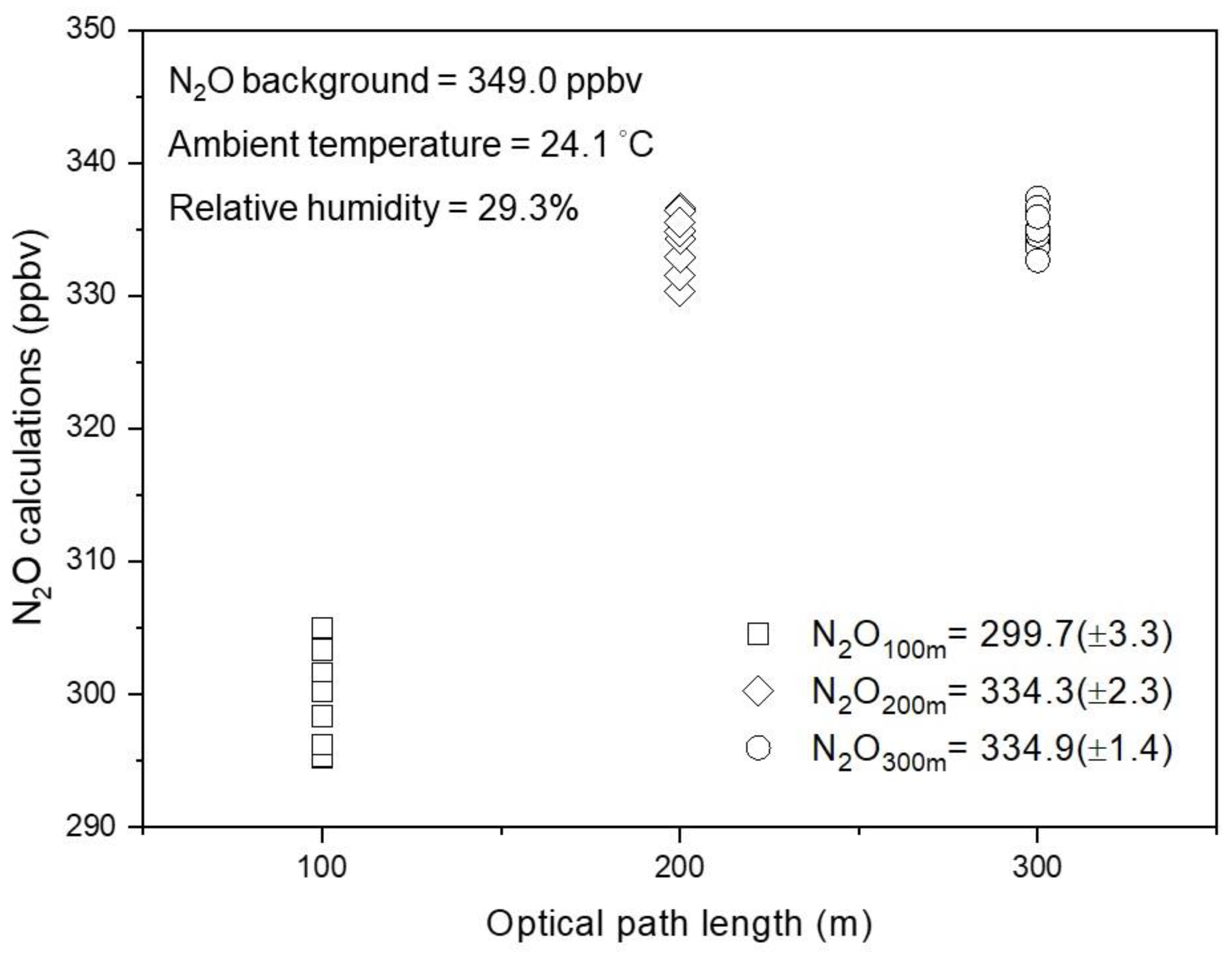
The LS N2O concentrations were derived from the measured OP-FTIR spectra. Both the precision and accuracy of N2O concentrations increased with increasing path lengths. Uncertainties in N2O concentrations (standard deviation) reduced from ±3.3 to ±1.4 ppbv by increasing optical path lengths from 100 m to 300 m (Figure 3). Nitrous oxide concentrations were underestimated by 14%, relative to the background concentration of 349.0 ppbv, at the optical path length of 100 m. By increasing path lengths to 300 m, the quantitative accuracy increased by approximately 10% (bias reduced from 14% to 4%). The increased path length increased the path-integrated concentrations (i.e., concentration × path length) as well as improved gas quantification [31]. Since the optical path lengths were between 200 (i.e., LS-2 and LS-6) and 300 m (i.e., LS-1, -3, -4, -5, and LS-7) in this scanning system, the uncertainties determined from the optical paths of 200 m (±2.3 ppbv) and 300 m (±1.4 ppbv) were averaged to calculate the overall uncertainty in N2O concentration of each LS sensor (i.e., ±1.8 ppbv). Concentration biases (~4%) were calibrated by the SOPS before flux calculations.
3.2. Emission Measurements
The influence of the TDF threshold for a valid bLS emissions estimate was evaluated relative to the potential for advective interference in the emissions estimate. We investigated the relationship between advective interferences (denoted by FRACair) and TDFs (Figure 4). The measured emissions were sorted into three categories based on the TDF threshold: high (>0.9), median (0.9 > TDF > 0.5), and low (0.5 > TDF > 0.1) to examine the relationships between emissions and TDFs (Figure 5).
3.2.1. High TDF Threshold (>0.9)
When the TDF values of the field of interest are nearly 1, the four treatments (T1–T4) alone had FRACair values (mean ± SD) of 89 ± 12%, 87 ± 14%, 84 ± 16%, and 80 ± 19% respectively (Figure 4). The targeted field received a “clean” upwind background and resulted in high TDFs (~1.0) when FRACair ~ 100%. For instance, T1 received a clean background when the wind came from SW (202.5–247.5°), as well as high TDFs (1.0) (Figure 4). Likewise, the SE wind (112.5–157.5°), NE wind (22.5–67.5°), and NW wind (292.5–337.5°) led the TDFs of 1.0 for T2, T3, and T4 treatments, respectively. Increased interference (0–20% of the FRACair of the adjacent upwind field) reduced TDFs from 1.0 to 0.9. For instance, T2 started interfering with T1 when the wind directions shifted from SW to S (~ 12% of FRACair from T2); likewise, T4 began to interfere with T1 at the direction of 270.0–292.5° (~ 6% of FRACair from T4) (Figure 4a). The mean (± SD) emissions of the T1 through T4 treatments were 3.9 ± 3.2, 0.8 ± 1.1, 1.5 ± 1.1, and 1.5 ± 2.1 µg m−2 s−1, respectively, over the 41 days of measurement (Figure 5). The uncertainty in N2O concentrations (±1.8 ppbv shown in Figure 3) was used to calculate the uncertainty in N2O emission rates, and the corresponding uncertainties in the emission estimates (mean ± SD) of the treatments T1 through T4 were 0.6 ± 0.2, 0.3 ± 0.1, 0.1 ± 0.1, and 0.5 ± 0.3 µg m−2 s−1, respectively (Figure 6). The emission rates indicated that the T1 treatment (i.e., the combination of NT and full N rates applied in the fall) resulted in the highest N2O emissions in the spring.
Negative emissions implied an N2O “sink”. Soil uptake of N2O, however, was unlikely when the soil was enriched with available N-substrates after NH3 application. One of the assumptions of the bLS model required a substantial difference in emission rates between the source (hotspot) and background to make the “delta concentration” detectable (Equation (1)). Negative emissions measured from a clean background and minimum interferences (TDF > 0.9 shown in Figure 5) were attributed to emissions lower than the detection limit. The standard deviation of the “negative” emissions of T1–4 (TDF > 0.9) was 0.4 µg m−2 s−1, so the MDL of this scanning open path method was calculated as ±1.2 µg m−2 s−1 (3σ) (gray bars shown in Figure 5).
3.2.2. Median TDF Threshold (0.9 > TDF > 0.5)
When the TDF values for the field of interest are median, the four treatments (T1–T4) alone had FRACair values (mean ± SD) of 52 ± 20%, 65 ± 19%, 43 ± 15%, and 40 ± 11%, respectively (Figure 4). The mean emission rates of the T1 through T4 treatments were 1.1 ± 1.9, −0.3 ± 1.6, 1.0 ± 2.2, and −1.2 ± 1.4 µg m−2 s−1, respectively (Figure 5). The emissions uncertainties (mean ± SD) were 0.8 ± 0.5, 0.4 ± 0.3, 0.3 ± 0.3, and 0.5 ± 0.4 µg m−2 s−1 for the T1 through T4 treatments, respectively (Figure 6). For TDF values between 0.5 and 0.9, the treatment plots of interest were interfered with by one predominant upwind treatment. For instance, the T2 treatment emissions strongly interfered with the T1 treatment for winds from 90° through 180° (Figure 4a). Interference from the T2 treatment emissions (FRACair increasing from 20% to 80%; shown in Figure 4a) reduced the TDFs of T1 from 0.9 to 0.5.
Adjacent field interference not only led to increased emissions uncertainty but also increased bias. The emissions bias became substantial if the upwind treatment emitted more than the downwind field. For instance, high N2O emissions were measured from T1 at the S wind (180–225°) (Figure 5a) substantially interfered with the T4 emissions measurements (with 60% of the FRACair from T1 shown in Figure 4d), resulting in “negative” emissions (less than the lower boundary of MDL of −1.2 ug m−2 s−1) from the T4 treatment (Figure 5d). Even when the TDF values were relatively high, the T1 treatment (upwind) emitted more N2O than T4 (downwind), so the air parcels from the T1 treatment likely carried higher N2O concentrations over the T4 plot (N2O advection) and introduced substantial biases in the downwind treatment emissions estimate. Emissions lower than −1.2 µg m−2 s−1 were considered as incorrect estimations and excluded.
3.2.3. Low TDF Threshold (0.5 > TDF > 0.1)
At low TDF threshold values, treatments of T1 through T4 alone only had relatively low FRACair values (mean ± SD) of 20 ± 5%, 16 ± 6%, 19 ± 6%, and 22 ± 5%, respectively (Figure 4). This indicated that the plot of interest was subject to substantial interferences from adjacent fields. The mean (± SD) emission rates of the T1 through T4 treatments were 0.2 ± 1.9, −1.2 ± 2.1, 3.0 ± 3.3, and −1.1 ± 1.4 µg m−2 s−1, respectively (Figure 5). The mean (±SD) in uncertainty in emissions for treatments T1 through T4 were 1.0 ± 0.4, 1.2 ± 0.4, 0.5 ± 0.5, and 1.0 ± 0.6 µg m−2 s−1, respectively (Figure 6). At higher threshold TDF values, the field of interest was typically interfered with by only one predominant upwind source. At low TDF, the increased FRACair (%) of multiple adjacent fields showed that more than two adjacent fields interfered with fields of interest (Figure 4). For example, the estimated emissions from the T1 treatment was influenced by the emissions from all the other treatments when the winds were from 0–90° (Figure 4a). Likewise, emissions from T2, T3, and T4 fields were interfered with by their neighbors when the wind came from the directions of 270–360°, 180–270°, and 90–180°, respectively (Figure 4). These “two-source” interferences corresponded with high emissions uncertainties (Figure 6).
At low TDF thresholds, the bias in adjacent field interference substantially influenced the field with low emission rates. For instance, emissions lower than −1.2 µg m−2 s−1 (lower bound of the MDL) were measured for T4 under an S wind because of the interferences from the T1 treatment emissions (Figure 4 and Figure 5). Emissions from the T3 treatment were subjected to interferences from the emissions from all the other treatments when the wind direction was 180–270° (prevailing SW wind in 2015 measurements). In contrast to the emissions from the T4 treatment, most of the emissions from the T3 treatment were still measurable and greater than the MDL (Figure 5c) even under the three-source interferences of the T1, T2, and T4 emissions.
3.3. Integrated Effects of Wind Direction and Speed
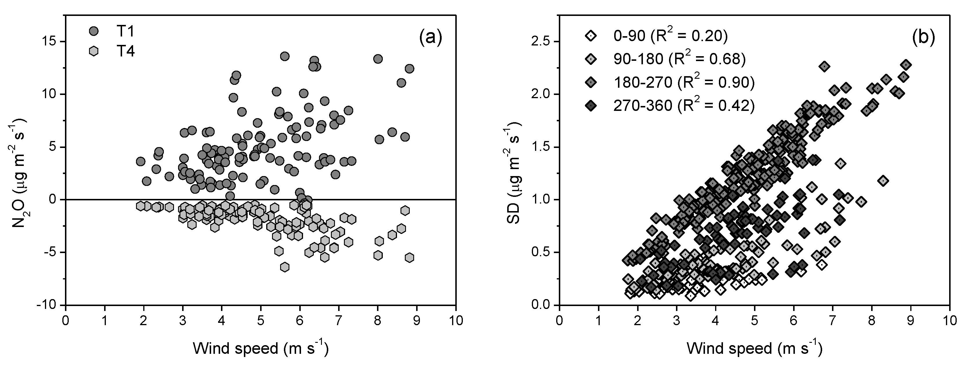
As expected, the adjacent field interference of the bLS-emission estimates was a function of the wind speed and direction. Increased wind speed resulted in greater bias (i.e., emissions < −1.2 µg m−2 s−1 shown in Figure 7a) and increased uncertainty (Figure 7b) in the emissions measurements. For instance, the increased wind speed amplified the interferences from T1 as well as emission biases for the T4 measurements at the S wind (Figure 7a). Advective interferences and the corresponding uncertainties in emissions were highly wind-speed-dependent. For instance, the NE wind (0–90) resulted in high TDFs (>0.9) and low uncertainties (0.1 ± 0.1 µg m−2 s−1) for T3 measurements. Interferences and emission uncertainties (0.5 ± 0.5 µg m−2 s−1) substantially increased at the wind from SW (180–270°) for T3 measurements. These uncertainties increased with increasing the wind speed: linear regression R2 value of 0.20 for winds from 0–90°; R2 = 0.68 for winds from 90–180°; R2 = 0.90 for winds from 180–270°; R2 = 0.42 for winds from 270–360° (Figure 7b).
Although this study only investigated the effect of uncertainties in N2O concentrations on the propagation of uncertainty in the bLS-measured emission, it is worthwhile to mention that the geometry of the source and sensor locations is another source of the uncertainties in bLS measurements [27,28,29]. Flesch et al. (2009) [29] mentioned that the source-sensor geometry is critical, and the ideal sensor deployment would be: each sensor only “sees” one emission source. The “optimal” deployment suggested by Flesch et al. (2009) [29] was also implemented in our study; however, the downwind sensors in the field of interest still detected the blended plume from the adjacent field via advection under different wind conditions. Therefore, the quantified advective interferences (Figure 4) associated with the propagated uncertainty in emission estimations (Figure 6) were used to assure data qualities in this study.
3.4. Data Filtering and Statistics
There was a total of 1968 possible half-hour bLS emission values (48 × 41 days) for each treatment over the period of 01 May to 11 June 2015. The OP-FTIR did not operate during intermittent rain events and field operations (e.g., herbicide spraying) due to the risk of FTIR mirror contamination, retroreflector contamination, or thermal IR signal absorption. The continuous operation was commonly impossible due to thermal IR signal absorption of condensed water on the spectrometer and/or retroreflector during the night or early morning. Strong wind-induced vibrations resulted in poor optical path alignment and low-quality OP-FTIR spectra resulting in poor N2O concentration estimation. Lastly, infrequent dusty wind-blown events also resulted in low spectra quality and N2O concentration determination. As a result, only 675 of the 1968 possible measurement periods (approximate 34%) were available to assess treatment effects on emissions in 2015.
Estimated emissions were excluded during ill-defined turbulence conditions of u* < 0.15 m s−1, |L| < 5 m, when TDF < 0.1, and when |N2Omin − | > 3σ ppbv (exclusion criteria 1 shown in Figure 8). Nearly 51% of the total collected half-hour emissions (n = 345 out of 675) remained for each treatment. Most of the excluded emissions were nighttime (i.e., 20:00–06:00, local time, LT) values when the boundary layer was stable with low winds. Estimated emissions less than the MDL (−1.2 µg m−2 s−1) were excluded due to the severe impact of the advection-induced bias (exclusion criteria 2 in Figure 8). An additional 62 and 101 half-hour periods of emissions were removed from analysis for the T2 and T4 treatments, respectively, mainly resulting from the predominant interference from the T1 plot under the prevailing SSW wind (Figure 1). For the T1 and T3 measurements, high emission plots, only 11 and 20 half-hour emissions were less than −1.2 µg m−2 s−1. Although emission estimations of the T3 treatment were interfered with by emissions from three adjacent fields (T1, T2, T4), most of the emissions from T3 were measurable (>MDL). The range of the advection-induced uncertainties was from 0.1 to 2.0 µg m−2 s−1 under different wind conditions and increased with increasing advective interferences (Figure 6). Estimated emissions were excluded if the uncertainty was 50% greater than the emission rates (exclusion criteria 3 shown in Figure 8). Low emissions, however, were more vulnerable to these criteria and excluded (Figure 8).
By excluding the data measured during the ill-defined turbulence conditions (exclusion 1), the mean N2O emissions of the four treatments over 41 day measurement period were 2.7 (T1), −0.2 (T2), 2.3 (T3), and −0.5 (T4) µg m−2 s−1, respectively (Figure 8). The mean “negative” emissions of the T2 and T4 treatments appeared to be largely due to the interference from T1 (Figure 5). These mean emissions became 2.8 (T1), 0.4 (T2), 2.5 (T3), and 0.4 (T4) µg m−2 s−1 by further removing the half-hour emissions less than −1.2 µg m−2 s−1 (exclusion 1&2), showing a substantial improvement for emission estimations from the T2 and T4 treatments. Exclusion criteria 3 reduced the measured emissions to only 24% of the total collected samples (n = 675). These left-over and relatively high emissions increased mean N2O emissions (i.e., 3.9 [T1], 0.7 [T2], 3.7 [T3], and 0.7 [T4] µg m−2 s−1) and likely overestimated the overall average emission rate over the measurement period. Therefore, we only implemented the exclusion criteria 1 and 2 to clean the data from each treatment. Moreover, the skewed distribution of the estimated emissions showed that the “instantaneous” high emissions substantially influenced the overall mean emission values. These high emissions were considered outliers (the value greater than the upper whiskers shown in Figure 8) and removed for population mean comparisons. The resulting mean N2O emissions were 2.3 (T1, n = 317), 0.3 (T2, n = 272), 2.1 (T3, n = 308), and 0.1 (T4, n = 232) µg m−2 s−1, corresponding to the mean N2O-N loss of 1.5 (T1), 0.2 (T2), 1.3 (T3), and 0.06 (T4) µg m−2 s−1.
3.5. Treatment Comparisons
The split-N rate application (T2) resulted in lower mean N2O emissions over the study period than the full-N rate application (T1) in the NT field (p < 0.05). This was consistent with the results of other studies [7,41,42,43]. For split N applications, chisel plowing the field before planting corresponded with higher mean N2O emissions in the growing season than when NT was done (T2 vs. T3, p < 0.05). This tendency for lower emissions under the NT management is consistent with the results of all prior N2O emission studies using soil chamber measurements at the ACRE [12,13,44]. The effect of tillage practices on N2O emissions are variable and based on climate regime and soil types [7,42,45]. This study suggested that NT management can mitigate N2O emissions, consistent with some field studies [42,46], but in contrast with others [47,48]. This inconsistency of the NT effect on N2O emissions may have been due to the duration of NT adoption. A long-term (>10 years) NT adoption was reported to mitigate N2O-N loss and the overall net global warming potential [42,48].
3.6. Flux Comparison with Other Studies
In this study, the quality-assured half-hour N2O emissions were observed from −1.2 to 15 µg m−2 s−1, corresponding to the N2O-N loss ranging from −0.8 to 9.5 µg m−2 s−1. By excluding outliers, the mean N2O-N emissions of four treatments were from 0.06 to 1.5 µg m−2 s−1. These emissions are comparable to the studies using the bLS method (or other inversion dispersion techniques) and other micrometeorological N2O flux studies. Based on the same measurement technique (OP-FTIR plus bLS), Bai et al. (2014 and 2018) [49,50] and Lam et al. (2015) [25,51] reported that the observed N2O-N emissions ranged from 1.7 to 7.5 µg m−2 s−1 with the mean N2O-N emissions from 0.8 to 1.7 µg m−2 s−1 over the study period from the N-fertilized soil. Flesch et al. (2016 and 2018) [24,52] also used OP-FTIR coupled with the bLS model to measure N2O-N emissions from cattle overwintering areas during the spring thawing (average soil temperature < 10 °C) and reported that the observed N2O-N emissions ranged from −0.5 to 4.2 µg m−2 s−1 with the daily mean N2O-N from 0.05 and 1.3 µg m−2 s−1. The bLS method has been extensively qualified in comparison with flux gradient [24], ZINST [53], mass balance [21], integrated horizontal flux method [54], and Eulerian inverse model [55], and these methods were in good agreement.
Compared with other micrometeorological studies measuring N2O emissions from cereal crop production systems [56,57,58], this study showed an increase in the estimated emission by a factor of 1.5~7. For instance, Tenuta et al. (2019) [56] and Machado et al. (2020) [57] used a closed-path gas concentration sensor coupled with the flux gradient method to measure N2O-N from N-fertilized croplands (e.g., corn, wheat, or barley) and observed N2O-N emissions ranging from 0 to 2.3 µg m−2 s−1. Cowan et al. (2020) [58] used the eddy covariance (EC) method to measure N2O-N emissions from the ammonium-nitrate- and urea-fertilized soils and showed the range of half-hour emission from 0 to 1.4 µg m−2 s−1. Not only do different N management practices significantly influence N2O emissions (Section 3.6), but the reduced N rate likely decrease emission rate [56]. These studies [56,57,58] usually had a lower annual total-N input from 98 to 180 kg-N ha−1 input with the mean N rate of 130 ± 28 kg-N ha−1 than this study (a total of 220 kg-N ha−1 annual input). Furthermore, soil microbes are sensitive to soil temperature, and the decreased temperature tends to reduce soil microbial activities as well as N2O productions. These studies [56,57,58] had a lower soil temperature (usually between 0 and 20 °C) during measurements than this study, which soil temperature was from 8.6 °C to 30.6 °C with the mean temperature of 18.2 ± 3.9 °C at the 10 cm soil (data not shown).
The EC method is one of the most common micrometeorological techniques often used to monitor long-term N2O-N loss and compare with the static chamber method. Several studies showed that EC and chamber methods had a similar flux magnitude for N2O-N measurements, but the EC method usually observed higher N2O-N emissions than chamber measurements [15,59,60]. The measurement of N2O fluxes by static and dynamic chambers has been more widely used to compare gas emissions among treatments and investigate the management effects on N2O emissions. Previous chamber studies cited in Section 3.6 [7,12,13,41,43,44,45,46,47,48] showed the mean emission values ranged from 0.01 to 0.32 µg m−2 s−1. Increased emissions measured using micrometeorological approaches are likely due partially to differences in the resistance to gas transfer through the still air in the soil pore space, through in the laminar layer of air over the soil, and through the turbulent boundary layer of air over the soil. Different soil gas permeability would then create differing resistances to gas flow in the soil, and differences in atmospheric turbulence would create differing resistance to gas flow in the turbulent atmosphere. Several studies showed increased wind speeds potentially increased N2O emissions, which was also shown in Figure 7a [16,61,62,63]. Poulsen et al. (2017) [62] and Pourbakhtiar et al. (2017) [63] indicated that the wind-induced emissions could be 20–100 times larger than the emissions that are only driven by the molecular diffusion (e.g., most of the chamber measurements).
3.7. Challenges and Potentials for Improvement
It is challenging to quantify the overall N2O-N loss over a long-term period (days to years) because of the high temporal variability in field N2O emissions. The OP-FTIR plus bLS system can measure gas fluxes with high temporal resolution and ideally have a better estimation for calculating the cumulative N2O-N loss. This method, however, could not measure emissions in low wind conditions commonly during nighttime (i.e., 20:00–06:00, LT, in this study) and had the potential for advective interferences under high wind conditions. For assessing “representative” cumulative N2O emissions, estimates of the emission during low and high wind conditions are required. Simply scaling up the mean emission using this method to estimate the overall N2O-N loss over the measurement period (e.g., conversion from µg-N m−2 s−1 to kg-N ha−1 over 41 days in this study) likely resulted in a substantial positive bias as well as misleading conclusion about the overall N2O-N loss. Although our studies showed that the scanning OP-FTIR plus bLS model could make “simultaneous” flux comparisons between treatments, the causes for the relatively high half-hourly emissions measured using this method need to be further studied.
For the method improvement, advective interference issues can be minimized by (1) adding measurements between treatments or reducing treatments, (2) measuring larger fields or by careful selection of adjacent treatments to prevent expected high and low emission treatments from interacting. Furthermore, the emission estimates under low wind conditions (e.g., largely nocturnal) must be included to evaluate long-term cumulative emissions, which can be achieved by incorporating different measurement techniques and appropriate “gap-filling” methods for missing data points [56,57,58]. For instance, chamber methods typically have a higher sensitivity to measure low emission rates than micrometeorological methods and can be operated in most weather conditions (e.g., rain events or low winds) [16]. Grant and Omonode (2018) [64] also showed that chamber measurements tend to be comparable to micrometeorological emission measurements during low winds and nocturnal conditions. The integrated uses of chambers and this or other micrometeorological methods would improve the temporal representativeness of seasonal to annual N2O-N loss estimations.
4. Summary and Conclusions
Measuring the above-canopy emissions in adjacent treatment plots was shown to require careful assessment of advection from adjacent fields. The commonly used threshold for sufficient sampling of an identified source (i.e., TDF > 0.1) in bLS modeling of emissions did not constrain the model conditions enough in this medium plot multi-source situation. In this study, TDF thresholds greater than 0.9 indicated that a field of interest received a clean upwind background and resulted in low emission uncertainties (0.5 ± 0.3 µg m−2 s−1) for N2O flux estimations. The TDF threshold values ranging from 0.5 and 0.9 typically had one predominant upwind field influencing the emission estimates of the downwind field of interest and increased emission uncertainties (i.e., 0.6 ± 0.4 µg m−2 s−1). The TDF thresholds less than 0.5 typically had all three fields contributing to upwind interferences and resulted in relatively high emission uncertainties (i.e., 1.1 ± 0.5 µg m−2 s−1). Under these conditions, the advection of N2O emitted from the upwind field likely negatively biased the downwind field emission estimations.
After minimizing this advective influence on the bLS-modeled emissions from the four adjacent fields, the effects of different N and tillage management practices on N2O emissions were generally consistent with prior studies based on soil-chamber emissions estimates. A single fall application of N led to higher growing season N2O emissions than the split-N rates applied in the fall and spring. For the same split-N applications in the fall and spring, the ChP practice tended to increase N2O emissions compared with the NT treatment.
Implementing the bLS method in a multi-source area is still ongoing research and becoming interesting to many users. Although the discrepancies in the presented values with other micrometeorological studies need to be further investigated, this study provides the current or future users with the approaches to identify the issues, potential solutions, and uncertainty analyses in a multi-source situation.
Author Contributions
Conceptualization, C.-H.L., R.H.G. and C.T.J.; data curation, C.-H.L.; formal analysis, C.-H.L.; funding acquisition, R.H.G. and C.T.J.; investigation, R.H.G. and C.T.J.; methodology, C.-H.L., R.H.G. and C.T.J.; project administration, R.H.G. and C.T.J.; resources, R.H.G. and C.T.J.; software, R.H.G.; supervision, R.H.G. and C.T.J.; validation, C.-H.L., R.H.G. and C.T.J.; visualization, C.-H.L.; writing—original draft, C.-H.L.; writing—review and editing, R.H.G. and C.T.J. All authors have read and agreed to the published version of the manuscript.
Funding
This research was funded by the United States Department of Agriculture National Institute for Food and Agriculture, USDA NIFA (grant no. 13-68002-20421); and the Indiana Corn Marketing Council (grant no. 12076053).
Acknowledgments
The authors appreciate the field management from Tony Vyn and Terry West, technical assistance and data collections from Austin Pearson and Allison Smalley, and the technical support from the United States Environmental Protection Agency (US EPA).
Conflicts of Interest
The authors declare no conflict of interest.
References
- Global Anthropogenic of Non-CO2 Greenhouse Gases Emissions: 1990–2030; EPA 430-R-12-006; United States Environmental Protection Agency: Washington, DC, USA, 2012. Available online: https://www.epa.gov/sites/production/files/2016-05/documents/epa_global_nonco2_projections_dec2012.pdf (accessed on 13 June 2020).
- Climate Change 2013: The Physical Science Basis. Working Group I Contribution to the Fifth Assessment Report of the Intergovernmental Panel on Climate Change; Cambridge University Press: Cambridge, UK; New York, NY, USA, 2013; Available online: https://www.ipcc.ch/report/ar5/wg1/ (accessed on 13 June 2020).
- Smith, P.; Martino, D.; Cai, Z.; Gwary, D.; Janzen, H.; Kumar, P.; McCarl, B.; Ogle, S.; O’Mara, F.; Rice, C.; et al. Greenhouse gas mitigation in agriculture. Philos. Trans. R. Soc. B-Biol. Sci. 2008, 363, 789–813. [Google Scholar] [CrossRef] [PubMed] [Green Version]
- Reay, D.S.; Davidson, E.A.; Smith, K.A.; Smith, P.; Melillo, J.M.; Dentener, F.; Crutzen, P.J. Global agriculture and nitrous oxide emissions. Nat. Clim. Chang. 2012, 2, 410–416. [Google Scholar] [CrossRef]
- Bouwman, A.F. Direct emission of nitrous oxide from agricultural soils. Nutr. Cycl. Agroecosyst. 1996, 46, 53–70. [Google Scholar] [CrossRef]
- Mosier, A.; Kroeze, C.; Nevison, C.; Oenema, O.; Seitzinger, S.; van Cleemput, O. Closing the global N2O budget: Nitrous oxide emissions through the agricultural nitrogen cycle. Nutr. Cycl. Agroecosyst. 1998, 52, 225–248. [Google Scholar] [CrossRef]
- Decock, C. Mitigating nitrous oxide emissions from corn cropping systems in the midwestern US: Potential and data gaps. Environ. Sci. Technol. 2014, 48, 4247–4256. [Google Scholar] [CrossRef]
- United States Department of Agriculture Economic Research Service (USDA-ERS). Available online: https://www.ers.usda.gov/data-products/fertilizer-use-and-price.aspx (accessed on 13 June 2020).
- Akiyama, H.; Yan, X.Y.; Yagi, K. Evaluation of effectiveness of enhanced-efficiency fertilizers as mitigation options for N2O and NO emissions from agricultural soils: Meta-analysis. Glob. Chang. Biol. 2010, 16, 1837–1846. [Google Scholar] [CrossRef]
- Snyder, C.S.; Bruulsema, T.W.; Jensen, T.L.; Fixen, P.E. Review of greenhouse gas emissions from crop production systems and fertilizer management effects. Agric. Ecosyst. Environ. 2009, 133, 247–266. [Google Scholar] [CrossRef]
- Venterea, R.T.; Maharjan, B.; Dolan, M.S. Fertilizer source and tillage effects on yield-scaled nitrous oxide emissions in a corn cropping system. J. Environ. Qual. 2011, 40, 1521–1531. [Google Scholar] [CrossRef] [Green Version]
- Omonode, R.A.; Kovács, P.; Vyn, T.J. Tillage and nitrogen rate effects on area- and yield-scaled nitrous oxide emissions from pre-plant anhydrous ammonia. Agron. J. 2015, 107, 605–614. [Google Scholar] [CrossRef]
- Omonode, R.A.; Vyn, T.J. Tillage and nitrogen source impacts on relationships between nitrous oxide emission and nitrogen recovery efficiency in corn. J. Environ. Qual. 2019, 48, 421–429. [Google Scholar] [CrossRef] [Green Version]
- Venterea, R.T.; Coulter, J.A.; Dolan, M.S. Evaluation of intensive “4R” strategies for decreasing nitrous oxide emissions and nitrogen surplus in rainfed corn. J. Environ. Qual. 2016, 45, 1186–1195. [Google Scholar] [CrossRef] [PubMed] [Green Version]
- Laville, P.; Jambert, C.; Cellier, P.; Delmas, R. Nitrous oxide fluxes from a fertilised maize crop using micrometeorological and chamber methods. Agric. For. Meteorol. 1999, 96, 19–38. [Google Scholar] [CrossRef]
- Denmead, O.T. Approaches to measuring fluxes of methane and nitrous oxide between landscapes and the atmosphere. Plant Soil 2008, 309, 5–24. [Google Scholar] [CrossRef]
- Schäfer, K.; Cellier, P.; Bertolini, T.; Dalgaard, T.; Weidinger, T.; Theobald, M.R.; Olesen, J.E. Spatial and temporal variability of nitrous oxide emissions in a mixed farming landscape of Denmark. Biogeosciences 2012, 9, 2989–3002. [Google Scholar] [CrossRef]
- Rowlings, D.W.; Grace, P.R.; Kiese, R.; Weier, K.L. Environmental factors controlling temporal and spatial variability in the soil-atmosphere exchange of CO2, CH4 and N2O from an Australian subtropical rainforest. Glob. Chang. Biol. 2012, 18, 726–738. [Google Scholar] [CrossRef]
- Flesch, T.K.; Wilson, J.D.; Yee, E. Backward-time Lagrangian stochastic dispersion models and their application to estimate gaseous emissions. J. Appl. Meteorol. 1995, 34, 1320–1332. [Google Scholar] [CrossRef] [Green Version]
- Flesch, T.K.; Wilson, J.D.; Harper, L.A.; Crenna, B.P.; Sharpe, R.R. Deducing ground-to-air emissions from observed trace gas concentrations: A field trial. J. Appl. Meteorol. 2004, 43, 487–502. [Google Scholar] [CrossRef] [Green Version]
- Yang, W.L.; Zhu, A.N.; Zhang, J.B.; Zhang, Y.J.; Chen, X.M.; He, Y.; Wang, L.M. An inverse dispersion technique for the determination of ammonia emissions from urea-applied farmland. Atmos. Environ. 2013, 79, 217–224. [Google Scholar] [CrossRef]
- Grant, R.H.; Boehm, M.T.; Bogan, B.W. Methane and carbon dioxide emissions from manure storage facilities at two free-stall dairies. Agric. For. Meteorol. 2015, 213, 102–113. [Google Scholar] [CrossRef]
- Huo, Q.; Cai, X.H.; Kang, L.; Zhang, H.S.; Song, Y.; Zhu, T. Estimating ammonia emissions from a winter wheat cropland in North China Plain with field experiments and inverse dispersion modeling. Atmos. Environ. 2015, 104, 1–10. [Google Scholar] [CrossRef]
- Flesch, T.K.; Baron, V.S.; Wilson, J.D.; Griffith, D.W.T.; Basarab, J.A.; Carlson, P.J. Agricultural gas emissions during the spring thaw: Applying a new measurement technique. Agric. For. Meteorol. 2016, 221, 111–121. [Google Scholar] [CrossRef]
- Lam, S.K.; Suter, H.; Davies, R.; Bai, M.; Sun, J.L.; Chen, D.L. Measurement and mitigation of nitrous oxide emissions from a high nitrogen input vegetable system. Sci. Rep. 2015, 5, 8208. [Google Scholar] [CrossRef] [PubMed] [Green Version]
- McBain, M.C.; Desjardins, R.L. The evaluation of a backward Lagrangian stochastic (bLS) model to estimate greenhouse gas emissions from agricultural sources using a synthetic tracer source. Agric. For. Meteorol. 2005, 135, 61–72. [Google Scholar] [CrossRef]
- Crenna, B.P.; Flesch, T.K.; Wilson, J.D. Influence of source–sensor geometry on multi-source emission rate estimates. Atmos. Environ. 2008, 42, 7373–7383. [Google Scholar] [CrossRef]
- Gao, Z.; Desjardins, R.L.; van Haarlem, R.P.; Flesch, T.K. Estimating gas emissions from multiple sources using a backward Lagrangian stochastic model. J. Air Waste Manag. Assoc. 2008, 58, 1415–1421. [Google Scholar] [CrossRef]
- Flesch, T.K.; Harper, L.A.; Desjardins, R.L.; Gao, Z.L.; Crenna, B.P. Multi-source emission determination using an inverse-dispersion technique. Bound. Layer Meteorol. 2009, 132, 11–30. [Google Scholar] [CrossRef]
- Lin, C.-H.; Grant, R.H.; Heber, A.J.; Johnston, C.T. Application of open-path Fourier transform infrared spectroscopy (OP-FTIR) to measure greenhouse gas concentrations from agricultural fields. Atmos. Meas. Tech. 2019, 12, 3403–3415. [Google Scholar] [CrossRef] [Green Version]
- Lin, C.-H.; Grant, R.H.; Heber, A.J.; Johnston, C.T. Sources of error in open-path FTIR measurements of N2O and CO2 emitted from agricultural fields. Atmos. Meas. Tech. 2020, 13, 2001–2013. [Google Scholar] [CrossRef] [Green Version]
- Hrad, M.; Piringer, M.; Kamarad, L.; Baumann-Stanzer, K.; Huber-Humer, M. Multisource emission retrieval within a biogas plant based on inverse dispersion calculations—A real-life example. Environ. Monit. Assess. 2014, 186, 6251–6262. [Google Scholar] [CrossRef]
- Huo, Q.; Cai, X.; Kang, L.; Zhang, H.; Song, Y.; Zhu, T. Inference of emission rate using the inverse-dispersion method for the multi-source problem. Agric. For. Meteorol. 2014, 191, 12–21. [Google Scholar] [CrossRef]
- Ro, K.S.; Johnson, M.H.; Hunt, P.G.; Flesch, T.K. Measuring trace gas emission from multi-distributed sources using vertical radial plume mapping (VRPM) and backward Lagrangian stochastic (bLS) techniques. Atmosphere 2011, 2, 553–566. [Google Scholar] [CrossRef] [Green Version]
- Ro, K.S.; Johnson, M.H.; Stone, K.C.; Hunt, P.G.; Flesch, T.; Todd, R.W. Measuring gas emissions from animal waste lagoons with an inverse-dispersion technique. Atmos. Environ. 2013, 66, 101–106. [Google Scholar] [CrossRef]
- Mukherjee, S.; McMillan, A.M.S.; Sturman, A.P.; Harvey, M.J.; Laubach, J. Footprint methods to separate N2O emission rates from adjacent paddock areas. Int. J. Biometeorol. 2015, 59, 325–338. [Google Scholar] [CrossRef]
- Flesch, T.K.; Wilson, J.D.; Harper, L.A.; Crenna, B.P. Estimating gas emissions from a farm with an inverse-dispersion technique. Atmos. Environ. 2005, 39, 4863–4874. [Google Scholar] [CrossRef]
- VanderZaag, A.C.; Flesch, T.K.; Desjardins, R.L.; Balde, H.; Wright, T. Measuring methane emissions from two dairy farms: Seasonal and manure-management effects. Agric. For. Meteorol. 2014, 194, 259–267. [Google Scholar] [CrossRef]
- Heber, A.J.; Ni, J.Q.; Lim, T.T.; Tao, P.C.; Schmidt, A.M.; Koziel, J.A.; Beasley, D.B.; Hoff, S.J.; Nicolai, R.E.; Jacobson, L.D.; et al. Quality assured measurements of animal building emissions: Gas concentrations. J. Air Waste Manag. Assoc. 2006, 56, 1472–1483. [Google Scholar] [CrossRef] [Green Version]
- SAS Institute. SAS/STAT 9.2 Users’s Guide; SAS Inst.: Cary, NC, USA, 2007. [Google Scholar]
- Robertson, G.P.; Vitousek, P.M. Nitrogen in agriculture: Balancing the cost of an essential resource. Annu. Rev. Environ. Resour. 2009, 34, 97–125. [Google Scholar] [CrossRef] [Green Version]
- van Kessel, C.; Venterea, R.; Six, J.; Adviento-Borbe, M.A.; Linquist, B.; van Groenigen, K.J. Climate, duration, and N placement determine N2O emissions in reduced tillage systems: A meta-analysis. Glob. Chang. Biol. 2013, 19, 33–44. [Google Scholar] [CrossRef]
- Burton, D.L.; Li, X.; Grant, C.A. Influence of fertilizer nitrogen source and management practice on N2O emissions from two Black Chernozemic soils. Can. J. Soil Sci. 2008, 88, 219–227. [Google Scholar] [CrossRef]
- Omonode, R.A.; Smith, D.R.; Gál, A.; Vyn, T.J. Soil nitrous oxide emissions in corn following three decades of tillage and rotation treatments. Soil Sci. Soc. Am. J. 2011, 75, 152–163. [Google Scholar] [CrossRef] [Green Version]
- Rochette, P.; Angers, D.A.; Chantigny, M.H.; Bertrand, N. Nitrous oxide emissions respond differently to no-till in a loam and a heavy clay soil. Soil Sci. Soc. Am. J. 2008, 72, 1363–1369. [Google Scholar] [CrossRef]
- Drury, C.F.; Reynolds, W.D.; Yang, X.M.; McLaughlin, N.B.; Welacky, T.W.; Calder, W.; Grant, C.A. Nitrogen source, application time, and tillage effects on soil nitrous oxide emissions and corn grain yields. Soil Sci. Soc. Am. J. 2012, 76, 1268–1279. [Google Scholar] [CrossRef]
- Liu, X.J.; Mosier, A.R.; Halvorson, A.D.; Zhang, F. The impact of nitrogen placement and tillage on NO, N2O, CH4 and CO2 fluxes from a clay loam soil. Plant Soil 2006, 280, 177–188. [Google Scholar] [CrossRef]
- Six, J.; Ogle, S.M.; Breidt, F.J.; Conant, R.T.; Mosier, A.R.; Paustian, K. The potential to mitigate global warming with no-tillage management is only realized when practised in the long term. Glob. Chang. Biol. 2004, 10, 155–160. [Google Scholar] [CrossRef] [Green Version]
- Bai, M.; Suter, H.; Lam, S.K.; Sun, J.L.; Chen, D.L. Use of open-path FTIR and inverse dispersion technique to quantify gaseous nitrogen loss from an intensive vegetable production site. Atmos. Environ. 2014, 94, 687–691. [Google Scholar] [CrossRef]
- Bai, M.; Suter, H.; Lam, S.K.; Davies, R.; Flesch, T.K.; Chen, D.L. Gaseous emissions from an intensive vegetable farm measured with slant-path FTIR technique. Agric. For. Meteorol. 2018, 258, 50–55. [Google Scholar] [CrossRef]
- Lam, S.K.; Suter, H.; Davies, R.; Bai, M.; Mosier, A.R.; Sun, J.L.; Chen, D.L. Direct and indirect greenhouse gas emissions from two intensive vegetable farms applied with a nitrification inhibitor. Soil Biol. Biochem. 2018, 116, 48–51. [Google Scholar] [CrossRef]
- Flesch, T.K.; Baron, V.S.; Wilson, J.D.; Basarab, J.A.; Desjardins, R.L.; Worth, D.; Lemke, R.L. Micrometeorological Measurements Reveal Large Nitrous Oxide Losses during Spring Thaw in Alberta. Atmosphere 2018, 9, 128. [Google Scholar] [CrossRef] [Green Version]
- Ni, K.; Koester, J.R.; Seidel, A.; Pacholski, A. Field measurement of ammonia emissions after nitrogen fertilization-A comparison between micrometeorological and chamber methods. Eur. J. Agron. 2015, 71, 115–122. [Google Scholar] [CrossRef]
- Yang, W.L.; Zhu, A.N.; Zhang, J.B.; Xin, X.L.; Zhang, X.F. Evaluation of a backward Lagrangian stochastic model for determining surface ammonia emissions. Agric. For. Meteorol. 2017, 234, 196–202. [Google Scholar] [CrossRef]
- Carozzi, M.; Loubet, B.; Acutis, M.; Rana, G.; Ferrara, R.M. Inverse dispersion modelling highlights the efficiency of slurry injection to reduce ammonia losses by agriculture in the Po Valley (Italy). Agric. For. Meteorol. 2013, 171, 306–318. [Google Scholar] [CrossRef]
- Tenuta, M.; Amiro, B.D.; Gao, X.P.; Wagner-Riddle, C.; Gervais, M. Agricultural management practices and environmental drivers of nitrous oxide emissions over a decade for an annual and an annual-perennial crop rotation. Agric. For. Meteorol. 2019, 276, 107636. [Google Scholar] [CrossRef]
- Machado, P.V.F.; Neufeld, K.; Brown, S.E.; Voroney, P.R.; Bruulsema, T.W.; Wagner-Riddle, C. High temporal resolution nitrous oxide fluxes from corn (Zea mays L.) in response to the combined use of nitrification and urease inhibitors. Agric. Ecosyst. Environ. 2020, 300, 106996. [Google Scholar] [CrossRef]
- Cowan, N.; Levy, P.; Maire, J.; Coyle, M.; Leeson, S.R.; Famulari, D.; Carozzi, M.; Nemitz, E.; Skiba, U. An evaluation of four years of nitrous oxide fluxes after application of ammonium nitrate and urea fertilisers measured using the eddy covariance method. Agric. Ecosyst. Environ. 2020, 280, 107812. [Google Scholar] [CrossRef]
- Jones, S.K.; Famulari, D.; Di Marco, C.F.; Nemitz, E.; Skiba, U.M.; Rees, R.M.; Sutton, M.A. Nitrous oxide emissions from managed grassland: A comparison of eddy covariance and static chamber measurements. Atmos. Meas. Tech. 2011, 4, 2179–2194. [Google Scholar] [CrossRef] [Green Version]
- Wang, K.; Zheng, X.H.; Pihlatie, M.; Vesala, T.; Liu, C.Y.; Haapanala, S.; Mammarella, I.; Rannik, U.; Liu, H.Z. Comparison between static chamber and tunable diode laser-based eddy covariance techniques for measuring nitrous oxide fluxes from a cotton field. Agric. For. Meteorol. 2013, 171, 9–19. [Google Scholar] [CrossRef] [Green Version]
- Maier, M.; Schack-Kirchner, H.; Aubinet, M.; Goffin, S.; Longdoz, B.; Parent, F. Turbulence effect on gas transport in three contrasting forest soils. Soil Sci. Soc. Am. J. 2012, 76, 1518–1528. [Google Scholar] [CrossRef] [Green Version]
- Poulsen, T.G.; Furman, A.; Liberzon, D. Effects of wind speed and wind gustiness on subsurface gas transport. Vadose Zone J. 2017, 16. [Google Scholar] [CrossRef]
- Pourbakhtiar, A.; Poulsen, T.G.; Wilkinson, S.; Bridge, J.W. Effect of wind turbulence on gas transport in porous media: Experimental method and preliminary results. Eur. J. Soil Sci. 2017, 68, 48–56. [Google Scholar] [CrossRef] [Green Version]
- Grant, R.H.; Omonode, R.A. Estimation of nocturnal CO2 and N2O soil emissions from changes in surface boundary layer mass storage. Atmos. Meas. Tech. 2018, 11, 2119–2133. [Google Scholar] [CrossRef]
Figure 1.
The experimental site was at the Purdue Agronomy Center for Research and Education (ACRE). The field experiment was operated by (a) a scanning OP-FTIR, and seven retroreflectors created seven line-sampling (LS) concentration sensors (LS-1–LS-7) to “scan” four treatments (T1–T4) managed by contrasting field and N practices shown in Table 1. Three point-sampling (PS) inlets were deployed at the edges of fields (W, N, and E) to measure the background N2O concentrations or provided additional downwind sensors for fields of interest. (b) The prevailing wind came from the SSW, and the mean wind velocity was 3.6 ± 1.8 m s−1.

Figure 2.
The procedure was used to estimate uncertainties in emission rates measured by the bLS model. Step 1: N2O concentrations of the seven line-sampling (LS) and three point-sampling (PS) sensors were “forward” calculated based on the known emission rates of the T1–T4 treatments. Step 2: two possibilities of the estimated concentrations with the introduced uncertainty (under- or overestimated) of the LS-1–LS-7 sensors were permuted. Step 3: 128 N2O emissions were “backward” calculated, and their standard deviation represented emission uncertainties at every 30 min interval.

Figure 3.
Open path FTIR spectra were acquired from optical paths of 100, 20, and 300 m and calculated for N2O concentrations. The mean concentration () and standard deviation (σ) represented the accuracy and uncertainties in the FTIR-calculated concentrations.
Figure 3.
Open path FTIR spectra were acquired from optical paths of 100, 20, and 300 m and calculated for N2O concentrations. The mean concentration () and standard deviation (σ) represented the accuracy and uncertainties in the FTIR-calculated concentrations.

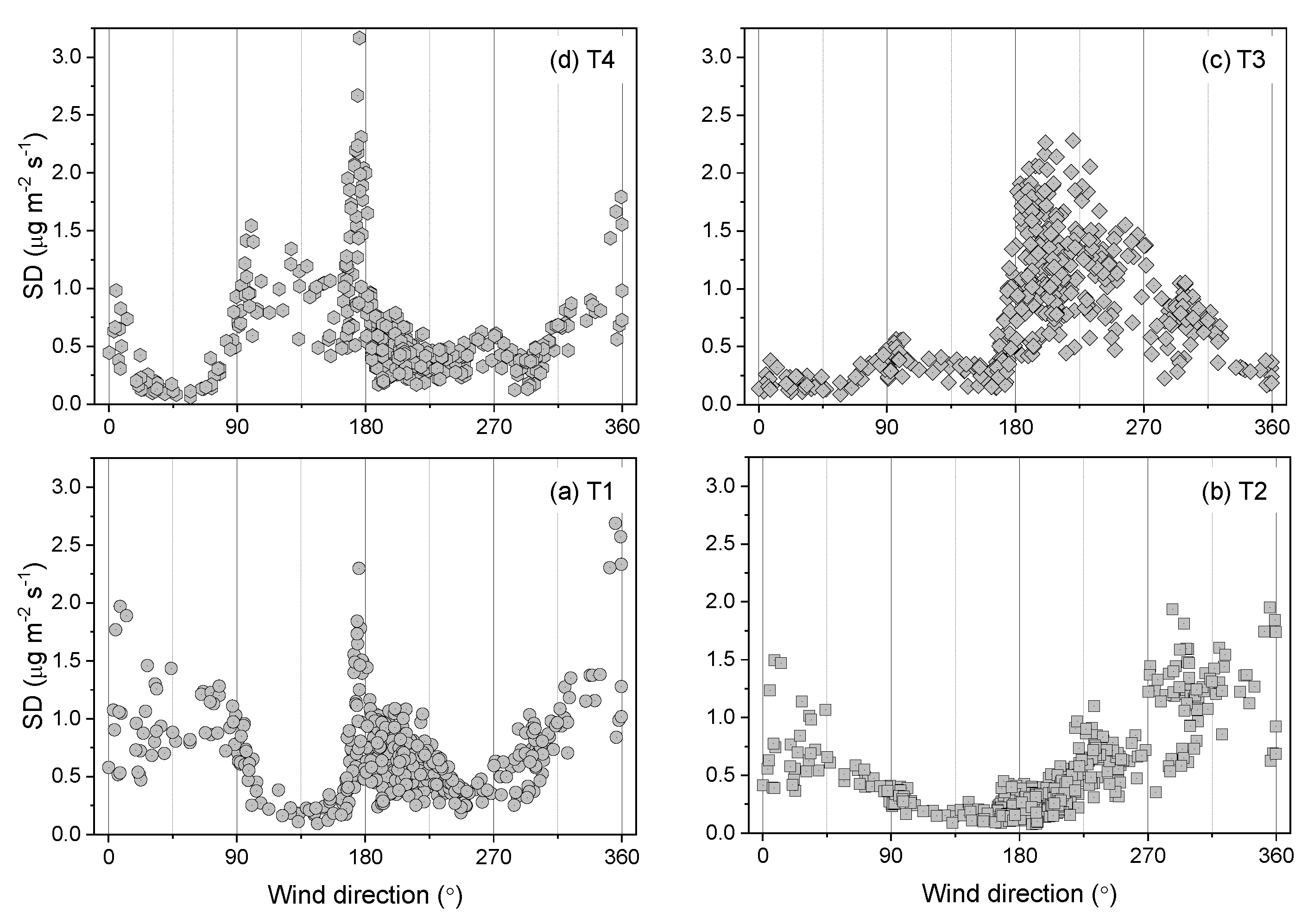
Figure 4.
The relationship between the “touchdowns” fraction (TDFs) of fields of interest: (a) T1, (b) T2, (c) T3, and (d) T4, and the interferences from the adjacent fields (shown as the fraction of air parcels, FRACair). For the field of interest, the FRACair traveling from adjacent fields was used to represent the magnitude of the upwind interferences.

Figure 5.
The relationship between the estimated emissions and the touchdowns fraction (TDFs) of fields of interest, (a) T1 (circle), (b) T2 (square), (c) T3 (diamond), and (d) T4 (hexagon). Emissions were classified into three categories of TDF > 0.9 (gray), 0.9 > TDF > 0.5 (light gray), and 0.5 > TDF > 0.1 (white).

Figure 6.
The uncertainties (shown as the standard deviation, SD) of the estimated N2O emission measurements from four treatments of (a) T1 (circle), (b) T2 (square), (c) T3 (diamond), and (d) T4 (hexagon) in this study. All symbols were with a dot in the center to differentiate from Figure 5.
Figure 6.
The uncertainties (shown as the standard deviation, SD) of the estimated N2O emission measurements from four treatments of (a) T1 (circle), (b) T2 (square), (c) T3 (diamond), and (d) T4 (hexagon) in this study. All symbols were with a dot in the center to differentiate from Figure 5.

Figure 7.
The effect of the mean wind speed on interferences from the upwind fields: (a) the T1 treatment interfered with the T4 treatment at the S wind, and these interferences increased with increasing the wind speed. Increased wind speed led to great biases (emissions < −1.2 µg m−2 s−1) in the T4 measurements; (b) the increased wind speed increased uncertainties (standard deviation, SD) in the T3 measurements.

Figure 8.
Stepwise criteria for data filtering and statistics of the remained fluxes (box plots and distributions) of four treatments: (a) T1 (dark gray circle), (b) T2 (gray circle), (c) T3 (light gray circle), and (d) T4 (white circle). Exclusion 1 was the ill-defined turbulence conditions (u* < 0.15 m s−1, |L| < 5 m, TDF < 0.1, and |N2Omin-| > 3σ ppbv). Exclusion 2 and 3 meant the advection-induced bias (emission less than −1.2 µg m−2 s−1, gray areas) and uncertainty ((, respectively. The box plot displays the mean (square), median (solid line), interquartile ranges (IQR between Q1 and Q3, box), and the boundaries for detecting outliers (upper: Q3 plus 1.5 × IQR and lower: Q1 minus 1.5 × IQR, whiskers).


Table 1.
Four treatments (T1–4) represented four N2O sources. Field practices were no-till and chisel plow. With the total N rate of 220 kg NH3-N ha−1, NH3 was applied as a full (220 kg N ha−1) or a split (total N rate was equally split and applied) application at two timings of the fall in 2014 and the spring before planting in 2015.
| Treatment (ha) | Tillage | Anhydrous Ammonia (Total = 220 kg NH3-N ha−1) | |
|---|---|---|---|
| 2014 Fall | 2015 Spring | ||
| T1 (1.2) | No-till | 220 | 0 |
| T2 (1.1) | No-till | 110 | 110 |
| T3 (1.1) | Chisel plow | 110 | 110 |
| T4 (1.2) | No-till | 0 | 220 |
Table 2.
An example of determining the fraction of air parcel (FRACair) that traveled from adjacent fields (i.e., T1, T3, and T4) to the field of interest (i.e., T2), representing the magnitude of interferences, under a particular wind condition (wind direction: NW (317°); mean wind velocity: 3.7 m s−1; friction velocity: 0.32 m s−1; Monin–Obukhov length: −37 m).
| Fields | Area (ha) | TDF | TD Cover † (ha) | Each Plot | TD Cover at Each Plot § (ha) | FRACair (%) |
|---|---|---|---|---|---|---|
| T2 | 1.5 | 0.24 | 0.36 | T2 | 0.36 | 17 |
| T2 + T1 | 2.7 | 0.28 | 0.76 | T1 | 0.40 | 19 |
| T2 + T3 | 2.9 | 0.32 | 0.93 | T3 | 0.57 | 27 |
| T2 + T4 | 2.6 | 0.43 | 1.12 | T4 | 0.76 | 36 |
TDF: touchdown fraction. TD cover †: touchdowns cover area for the specified field, calculating by multiplying the area (e.g., 2.9 ha) by TDF (e.g., 0.32) of the specified field (e.g., T2 + T3). §: TD cover at each plot was calculated based on the difference of the TD cover area between specified fields. For example, TD cover areas of T2 only and T2 + T3 were 0.36 and 0.93, respectively. Thus, the TD cover area of T3 only was 0.57 (i.e., 0.93 subtracted 0.36). FRACair (%): a fraction of air parcels, the percentage of TD cover area at each plot among four plots (treatments).
Publisher’s Note: MDPI stays neutral with regard to jurisdictional claims in published maps and institutional affiliations. |
© 2020 by the authors. Licensee MDPI, Basel, Switzerland. This article is an open access article distributed under the terms and conditions of the Creative Commons Attribution (CC BY) license (http://creativecommons.org/licenses/by/4.0/).
Share and Cite
MDPI and ACS Style
Lin, C.-H.; Grant, R.H.; Johnston, C.T. Measuring N2O Emissions from Multiple Sources Using a Backward Lagrangian Stochastic Model. Atmosphere 2020, 11, 1277. https://0-doi-org.brum.beds.ac.uk/10.3390/atmos11121277
AMA Style
Lin C-H, Grant RH, Johnston CT. Measuring N2O Emissions from Multiple Sources Using a Backward Lagrangian Stochastic Model. Atmosphere. 2020; 11(12):1277. https://0-doi-org.brum.beds.ac.uk/10.3390/atmos11121277
Chicago/Turabian StyleLin, Cheng-Hsien, Richard H. Grant, and Cliff T. Johnston. 2020. "Measuring N2O Emissions from Multiple Sources Using a Backward Lagrangian Stochastic Model" Atmosphere 11, no. 12: 1277. https://0-doi-org.brum.beds.ac.uk/10.3390/atmos11121277
Note that from the first issue of 2016, this journal uses article numbers instead of page numbers. See further details here.