Local and Remote Sources of Airborne Suspended Particulate Matter in the Antarctic Region


1
Laser Lab, Chemistry & Environment Group, Department of Analytical Chemistry, Faculty of Sciences, University of Zaragoza, Pedro Cerbuna 12, 50009 Zaragoza, Spain
2
Laser Chemistry Research Group, Department of Analytical Chemistry, Faculty of Chemistry, Complutense University of Madrid, Plaza de Ciencias 1, 28040 Madrid, Spain
*
Author to whom correspondence should be addressed.
Atmosphere 2020, 11(4), 373; https://0-doi-org.brum.beds.ac.uk/10.3390/atmos11040373
Submission received: 29 March 2020
/
Revised: 6 April 2020
/
Accepted: 8 April 2020
/
Published: 10 April 2020
(This article belongs to the Special Issue Sources and Composition of Ambient Particulate Matter)
Abstract
:Quantification of suspended particulate matter (SPM) measurements—together with statistical tools, polar contour maps and backward air mass trajectory analyses—were implemented to better understand the main local and remote sources of contamination in this pristine region. Field campaigns were carried out during the austral summer of 2016–2017 at the “Gabriel de Castilla” Spanish Antarctic Research Station, located on Deception Island (South Shetland Islands, Antarctic). Aerosols were deposited in an air filter through a low-volume sampler and chemically analysed using Inductively Coupled Plasma-Mass Spectrometry (ICP-MS) and Inductively Coupled Plasma-Atomic Emission Spectroscopy (ICP-AES). Elements such as Al, Ca, Fe, K, Mg, Na, P, S, Cu, Pb, Sr, Ti, Zn, Hf, Zr, V, As, Ti, Mn, Sn and Cr were identified. The statistical tools together with their correlations (Sr/Na, Al/Ti, Al/Mn, Al/Sr, Al/Pb, K/P) suggest a potentially significant role of terrestrial inputs for Al, Ti, Mn, Sr and Pb; marine environments for Sr and Na; and biological inputs for K and P. Polar contour graphical maps allowed reproducing wind maps, revealing the biological local distribution of K and P (penguin colony). Additionally, backward trajectory analysis confirmed previous affirmations and atmospheric air masses following the Antarctic circumpolar pattern.
1. Introduction
The Antarctic region is considered to be one of the most virgin, isolated and remote areas globally. The Antarctic is a polar desert and acts as a global thermostat, controlling the global climate system. Nevertheless, although this area is well distanced from continental regions, anthropogenic aerosol pollution from remote and local sources negatively affects the Antarctic environment [1]. Besides, a growing number of tourists visit Antarctica every year. Port Foster, situated in the caldera of Deception Island, is the second most-visited site in this continent, with more than 20,000 visitors in the 2016–2017 austral summer season [2].
Atmospheric aerosols act as climate drivers, since they are involved in the radiation balance of the Earth [3] and the formation of clouds [4]. However, aerosol studies regarding their origin and interactions are still limited and unclear [5]. Aerosols are produced by natural sources (sea, earth erosion, biogenic emissions, volcanoes, etc.) and anthropogenic sources (fossil fuel combustion, mining, agriculture, etc.), negatively affecting the Antarctic’s air quality and ecosystems. Thus, it is important to study them and their impacts on the environment [6].
Atmospheric aerosols have a typical lifetime of one day to two weeks in the troposphere [5]. They transform their size and distribution as they evolve [7], affecting remote places such as the Antarctic [8]. Particulate Matter (PM) transport depends on the wind and meteorological conditions [9,10]. This is important, since the Antarctic region is known for being a trap for aerosols from other places [11].
Air mass back trajectories are precise tools used for investigating the source of the pollutants [12] by estimating the flow patterns of air arriving at the sample collection point. Back trajectory analyses allow for the tracking of the source of aerosols emissions. Long-distance back trajectories are influenced by physical and chemical processes (e.g., deposition and advection), while short-distance trajectories are influenced by emission source zones [13]. However, position inaccuracies of up to 20% of the travel distance can exist [14]. As much as 30% of chemical variability in the troposphere can be associated with transport [15].
Through multivariate analysis, Pérez-Arribas [16] studied a large set of air quality data, aiming to identify elemental correlations and their shared origin. Modelling relationships are important tools to study the relationships between different analytical data, allowing the reproduction of temporal and spatial variations [17,18].
Chemical PM composition has been previously studied in the Antarctic [19]. Nevertheless, despite the importance of PM origin, limited publications using air mass back trajectories exist regarding the Antarctic region [20,21,22].
The aim of this study is to gain better insight into the potential natural or anthropogenic sources of the measured particulate matter composition and concentration, through air mass back trajectories and polar contour maps. Furthermore, a combination of statistical and graphical approaches is proposed to establish the relationship between the elements and their concentration, in order to reveal the influence of marine environments, human-made activities and penguin colonies on the Antarctic region.
2. Materials and Methods
2.1. Site Description and Sampling
The site description, sampling procedure, and methodology used in the present work, along with the most significant experimental conditions, have been previously described elsewhere [6]. Thus, only the more relevant information to this study is presented here. Atmospheric aerosol particles were collected during the austral summer (from December 2016 to February 2017) at Deception Island (Figure 1), at the Spanish Antarctic Research base “Gabriel de Castilla” (62°58′09″ S, 60°42′33″ W). A total of 37 samples were collected in circular quartz filter paper of 47 mm diameter (Munktell) by a Derenda LVS 3.1 low volume sampler (2.3 m3/h), and after 24 h, were placed by hand into sterile Petri dishes using sterile tweezers and nitrile globes. Mass concentration was obtained by gravimetry following the European Norm [23]. Additionally, soil samples were taken from the area of interest. After the gravimetric analysis, Hf, Zr, V, As, Ti, Mn, Cu, Sn, Zn and Pb were determined using Inductively Coupled Plasma-Mass Spectrometry (ICP-MS) and Inductively Coupled Plasma-Atomic Emission Spectroscopy (ICP-AES), as previously described in another publication [6].
2.2. Data Processing
Correlation analysis is a statistical method used to provide information about the relationship between elements that form the air PM by means of a mathematical model. Zhu [24] studied the sources of chemical constituents using multidimensional analysis. The study established correlations between the elements in aerosols. Additionally, a principal component analysis (PCA) was used as an element position simplification tool. Pérez-Arribas [16] adopted PCA to allow a group of correlated data to be transformed into a reduced coordinate system. In this study, Statgraphics Centurion 18, version 18.1.06 of 64-bits (Statpoint Technologies, Warrenton, VA, USA) was used for executing the correlation analysis and the principal component analysis (PCA).
2.3. Polar Contour Maps
OriginPro 2017, 64-bit (OriginLab Corporation, Northampton, MA, EEUU) was used for studying data relationships through Polar contour maps. These were used as an effective tool for local data visualization. The use of wind direction and speed provided an easy and useful plot of air-pollutants sources. The wind speed is displayed on the x-axis, wind direction on the y-axis of the angle (the radius in degrees), and concentration on the z-axis.
2.4. Air-Mass Back Trajectories
Aiming to distinguish potential remote natural and anthropogenic sources at the sampling location, ten days of air-mass backward trajectories were implemented for an endpoint 600 m above ground level (AGL). This height was selected since the mountainous island has a circular form, and the highest altitude (Mount Pond) is 542 m. In this study, diverse models were used to calculate backward trajectories. Nevertheless, Cabello and Harris [25] pointed out that there are discrepancies between trajectories obtained with different models and different vertical transport methods. The trajectories were calculated with the NOAA HYSPLIT4 (Hybrid Single Particle Lagrangian Integrated Trajectory) model [12,26]. GDAS 1 degree (Global Data Assimilation System) meteorological data from the National Weather Service’s National Centre for Environmental Prediction (NCEP) were chosen as the best appropriate trajectory model over those that did not cover the investigated region and had lower-resolution. GDAS has been widely used to perform backward air trajectories in locations other than the Antarctic region [27,28,29,30].
3. Results and Discussion
3.1. Statistical Description of the Data Normality Tests
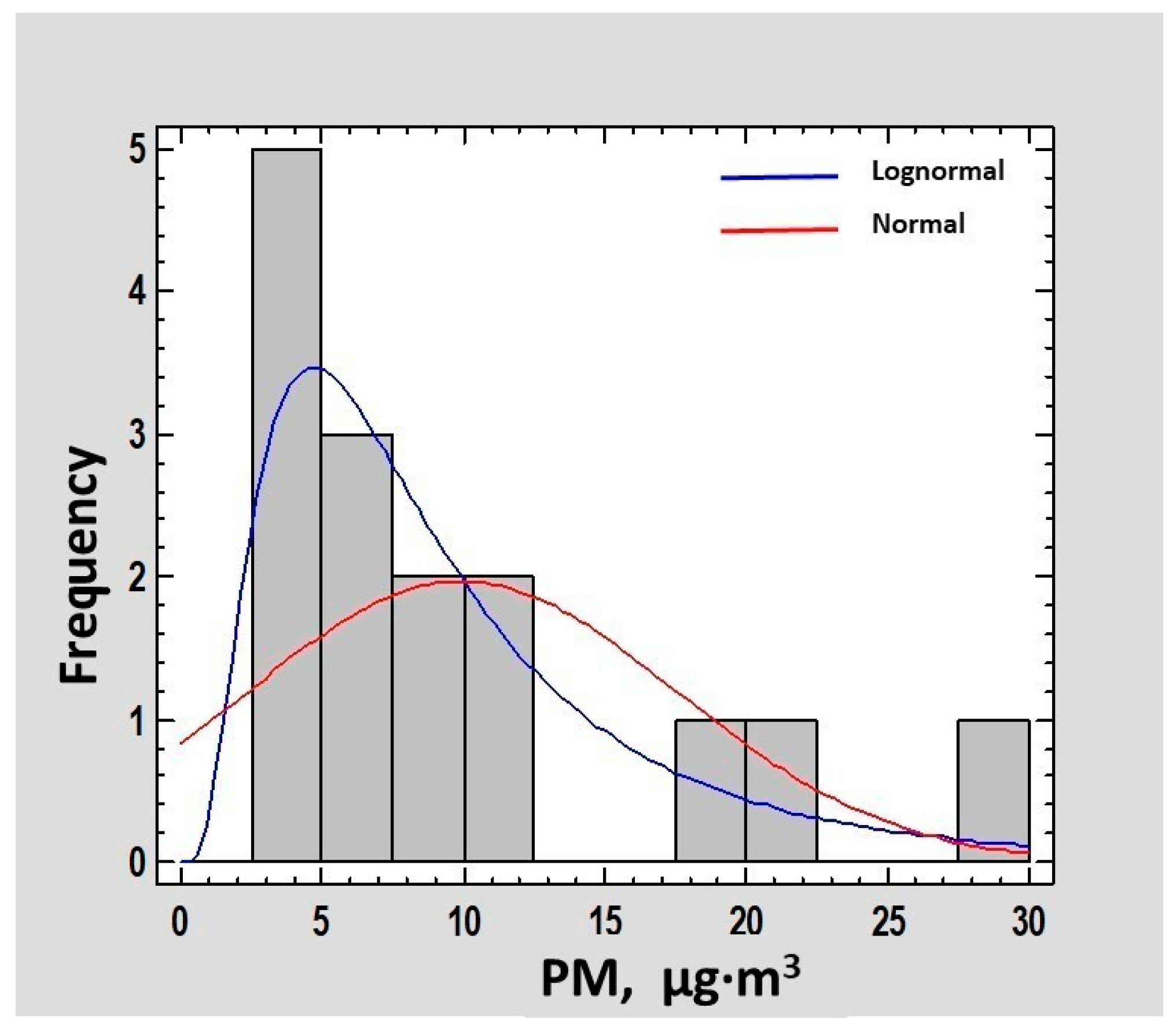
Particulate matter results show an average of 10 ± 4 μg/m3. This value is similar to those found in low population density areas and places such as the Southern Ocean (13.4 μg/m3; [31]). However, this result differs from other values found on the Antarctic coast with an average of 1.5 μg/m3 or 3.4 μg/m3 [32,33]). The statistical analysis result of total particulate matter (PM10) is shown in Table 1. The results show a great variability between the sampling days, ranging from 2.9 to 28.2 µg/m3 with a variation coefficient of 76.4%. The variability is explained by the singular shape of Deception Island (mountainous horseshoe). This peculiar shape keeps aerosols in the air for an extended period of time.
Both standard skewness and standard kurtosis can be used to determine if the sample has a normal (Gaussian) or different statistical distribution. In general, statistical values outside the range of −2 to + 2 indicate significant deviations from normality, which would tend to invalidate many of the statistical procedures that are usually applied to these data.
It can be seen in Table 1 and Figure 2 that the distribution of PM10 data indicates a certain asymmetry, although not well above the critical value of two. Positive asymmetry is usually an indication of a logarithmic-normal or lognormal type of distribution of data. To verify this possibility, the Kolmogorov–Smirnov test was carried out, with the P-value estimated for a possible lognormal distribution of 0.9983 and 0.6100 estimated for the normal one. Seeing as the two probability values calculated are above the level of usual significance (α = 0.05), both statistical distributions are statistically valid. However, as can be seen in Figure 2, the lognormal distribution is better suited to the PM10 data obtained. Figure 2 shows a representation of the distribution of number of days (frequency) and PM concentration (μg/m3).
Once the general PM statistical behaviour was studied, the same procedure was applied to the different pollutants found in PM10. Specific elements found in the aerosol also showed great variability between different sampling days. However, this variability was not homogeneous for all of them, as shown in Table S1 (Supplementary Materials).
Most of the elements have variation coefficients between 100% and 50%, similar to the PM10 variation coefficient of 76.4%. However, some elements show variation coefficients which are very different and higher than this value. Airborne PM is often affected by different climatic conditions (wind direction, speed, humidity, precipitation, etc.). This implies that, generally, the behaviour of PM composition follows the same trends, but this does not occur for some elements such as; P, K and Sn, with coefficient of variation (C.V.) of 249%, 169.9% and 124.5%, respectively; and for Cu and Fe, with C.V. of 112% and 102%, respectively. This means that these elements may be related to emission sources relatively close to the collection place and possibly very localized, probably due to very intense emission sources. Generally, this situation occurs when the distribution changes from normal or Gaussian statistical behavior, to strong positive asymmetry (lognormal distribution). In the case of K and P, its Kolmogorov–Smirnov test is shown in Table 2 compared to their Gaussian distribution.
In both cases, the P-value for a normal distribution is <0.05, indicating that the contents of K and P in the particulate material are not distributed over the sampling days according to a Gaussian model, and that the lognormal distribution model is much more suitable to describe the behaviour of these major elements. Regarding the trace elements found in the Antarctic aerosol, Cu shows marked positive asymmetry, although in this case, its distribution over the days of sampling can be explained both by a normal model and by a lognormal model, since the fit tests show P-value > 0.05 on both models.
3.2. Correlation Analysis
Aiming to explore the chemical/environmental associations among the elements found in the PM10, correlation analysis has been carried out. A statistically significant correlation between elements indicates a common origin of both, so if the source of one of them is identified, it can be presumed that the other comes from the same source of emission. Statistically significant correlations were found between the major constituents in the PM10 [6] and in the case of the elements present at trace levels, 6 significant correlations were found between them [21]. However, it is unknown if some trace elements are correlated to any of the major components. Table S2 (Supplementary Materials) shows the analysis of correlations corresponding to the elements found in the aerosol during the campaign. Those elements that show significant correlation (P-value < 0.05) are shown in shaded cells.
As Table S2 (Supplementary Materials) shows, there is a very significant correlation between Sr and Na (Pearson = 0.9873 and P-value < 0.0001). Since the main source of Na in the particulate material is marine aerosol, this implies that Sr also has a marine origin. The remaining trace elements do not show a significant correlation with Na, so the marine origin of these elements is discarded. Moreover, Al is a characteristic element of the earth’s crust. Al and Ti have a very significant, high correlation (Pearson 0.9430; P-value < 0.0001). Therefore, Ti has a crustal origin as well. Along with its marine origin, Sr has a correlation with Al (Pearson 0.5979; P-value = 0.0240). This indicates that some Sr has a terrestrial input. Other trace elements present in the aerosol with possible terrestrial origin are Mn (Pearson 0.8635; P-value = 0.001) and Pb (Pearson 0.7557; P-value 0.0028).
3.3. Multivariate Analysis
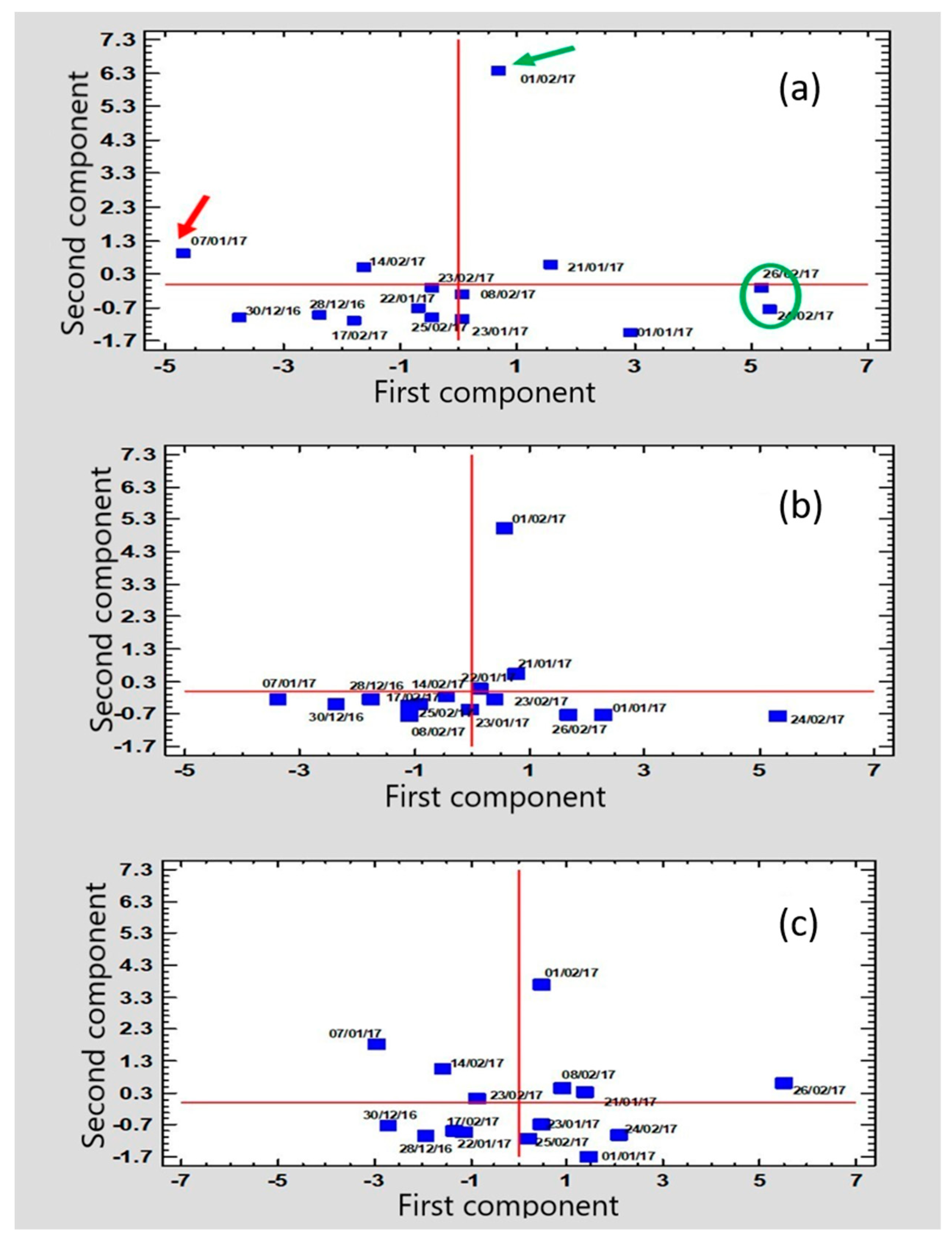
Previous correlation analysis has described that there are significant correlations (P-value < 0.05) among some of the elements found in the PM10. Subsequently, PCA has been carried out, aiming to check if these relationships occur globally. Figure 3 shows the scatter diagrams corresponding to the sampling days. Figure 3a presents the scatter plot when all elements found have been computed as variables; in Figure 3b, the dispersion diagram corresponds to the majority of the elements and Figure 3c corresponds to the components that are at trace levels. Given that the elements were found in different concentration levels, the PCA has been carried out after scaling the data by standard deviation (autoscaling). The green circle indicates that there are two values (samples) close to each other, and therefore there is some similarity between them. However, at the same time, these values are different from the rest. The green and red arrows indicate the same, values that are out of the guideline or general behavior.
As can be seen in Figure 3, the distribution of the scores are quite similar. Most of the points are located at the bottom of the diagram and close to the origin of coordinates. This means that the different pollutants maintain a similar pattern. However, there are exceptions. Figure 3a shows that the sample taken on 1 February 2017 is separated from the rest of the points. This indicates that there is a different pattern compared to the rest of the samples. Similarly, this occurs in Figure 3b,c.
The different patterns show the occurrence of K and P (major elements); and V and as (trace elements). These elements are significantly correlated with each other (see correlation Table S2 in Supplementary Materials). The maximum values of these elements were measured on 1 February 2017, while the rest of the elements gave values close to or below the average. On the other hand, these elements do not show a significant correlation with either Na or Al, so their marine or crustal origin is discarded.
It can be observed in Figure 3a that for two days (24 February 2017 and 26 February 2017) the elemental composition differs, in relative terms, from the rest of the days. Even though these days appeared close on the distribution diagram, they have different characteristics. One of them corresponds to the presence of majority elements and the other to trace elements. The highest concentration levels were recorded on 24 February 2017 (Figure 3b). The majority elements concentration was recorded to be above the average, except for K and P, on 26 February 2017 (Figure 3c). On this day, a similar situation happened with minority elements, with the exception of V and as (Table S1, Supplementary Materials).
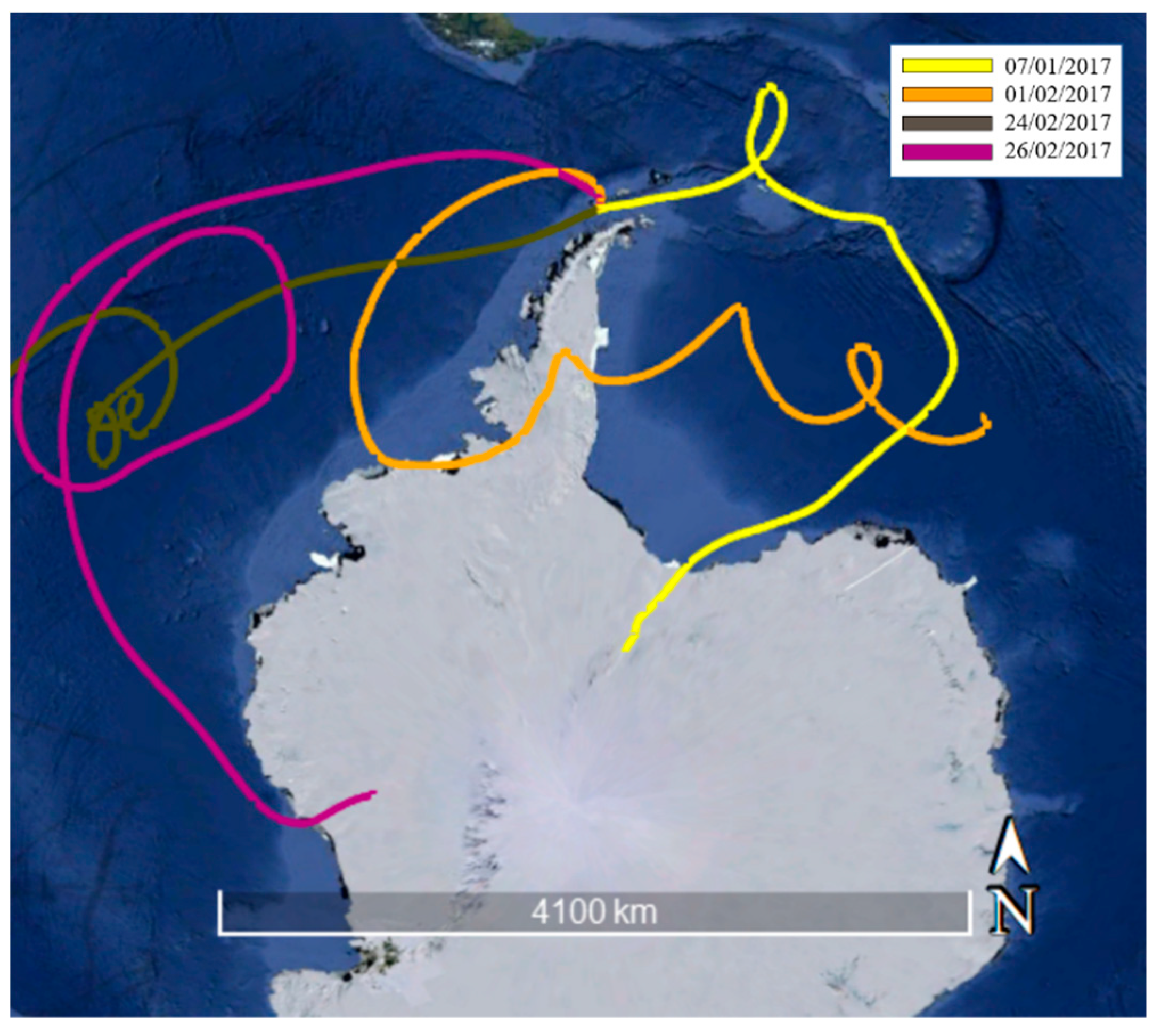
Finally, the point associated to PM collected on 07 January 2017 also deviates from the general pattern. However, this point should be considered anomalous or unrepresentative, since on that day, Fe, Mn, Zn, Sn and Hf were not detected. Furthermore, the rest of the elemental concentration was minimum or largely below the average. Some of these facts could be explained based on the air mass backward trajectories associated with the days prior to the sampling or the sampling meteorological conditions (Figure 4). Generally, air mass backward trajectory analysis showed that PM10 moved following the Antarctic Circumpolar Pattern through the Southern and Pacific Oceans, while for some of the cases air masses originated close to the Antarctic Peninsula at the Weddell and Bellingshausen Seas.
- Air mass backward trajectories associated to 01 February 2017 (Figure 4) show previous winds to this day with origin on the Weddell Sea, passing through the Antarctic continent and the Bellingshausen Sea. These areas are mostly covered by ice and snow. This explains the low concentration levels of crustal or marine elements.
- Backward trajectories associated to 24 February 2017 and 26 February 2017 (Figure 4) show previous days were similar, although on the 26th wind travelled through areas farther north than on the 24th. In both cases, the wind route passed mainly through ice-free areas, so these days prevail the presence of Na and the elements correlated with it, such as Mg. In addition, on 26 February 2017 there was moderate rainfall and high relative humidity, which favoured the deposition of the aerosol.
- On 07 January 2017 (Figure 4), very low levels of all the elements were detected. This cannot be explained either by the air mass backward trajectories or by the sampling weather conditions. Therefore, it should be considered to be anomalous.
3.4. Polar Contour Maps
In the statistical study of the pollutant’s distribution, it was found that K and P did not show Gaussian distribution. However, their distribution was a positive asymmetric lognormal type. This type of distribution is relatively frequent in the environmental analysis, mainly when there are high intensity emission sources, relatively close to the sampling site. These sources are usually located somewhere very localized.
Since the transport of pollutants in the air is carried out by the wind, polar contour maps were used to relate the concentration of these pollutants in the air with wind direction and speed. On the other hand, according to the correlation study mentioned above, K and P have an important and significant correlation between them (Pearson 0.9821; P-value < 0.0001). Alternatively, they do not present a significant correlation with either Na or Al. This indicates that both elements have the same non-crustal, marine origin.
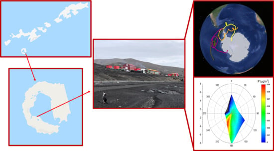
If we look at the polar contour maps associated to these two elements (Figure 5), the emission focus of both maps is in the 210° direction (south-west of the sampling site). This implies a natural and biological origin of these elements, since the Punta de la Descubierta penguin colony is located in that direction. This colony is one of the largest penguin colonies in Deception Island, so the presence of these elements in the PM is related to the excrement (guano) in the area.
4. Conclusions
By using statistical methods combined with polar contour Maps and air mass back trajectories, the different sources of PM collected during the austral summer campaign in 2016–2017 (2.5-month term) at the Spanish Antarctic Research Base “Gabriel de Castilla” located on Deception Island have been determined.
Correlation analysis between major and minor elements showed the potential source of the airborne PM. Sr/Na correlation indicated the influence of marine aerosols, whereas Al/Ti correlation revealed the influence of local crustal sources. Al/Mn, Al/Sr and Al/Pb correlations indicated terrestrial sources. Furthermore, K/P correlation was revealed to have non-crustal/marine origins, since no correlation with Na or Al was found. Multivariate analysis proved the importance of establishing guidelines in the behaviour of PM10 and its composition throughout the sampling period. Score distribution showed a similar pattern for most of the elements, except for K and P. The origin of the K/P correlation was validated by PCA and polar contour maps to be biological (penguin scats from the penguin colony).
Air mass back trajectories were used to confirm the elemental source. These trajectories revealed that both crustal and marine inputs occurred following different pathways and were influenced by the Antarctic Circumpolar pattern.
This work revealed the importance of an improved understanding of the potential origin and behaviour of PM in the Antarctic, through the use of statistical tools, air mass back trajectories and polar contour maps. Consistent aerosol tracking in the Antarctic region is crucial, since atmospheric aerosols play a significant role in the Earth´s climate and ecosystems. Further work will be undertaken on Deception Island as well as at other Antarctic stations.
Supplementary Materials
The following are available online at https://0-www-mdpi-com.brum.beds.ac.uk/2073-4433/11/4/373/s1. Table S1: Statistical summary of major (a; µg/m3) and minor elements (b; ng/m3). Those elements that show significant deviation from the Gaussian model (statistical values outside the range −2 to +2) are in red., Table S2: Statistics of correlations between different elements. For each element the first, second and third row correspond to Pearson correlation coefficient, sample size and P-Value, respectively. Those elements that show significant correlation (P-value <0.05) are shown in shaded cells.
Author Contributions
C.M.-M.: Writing-original draft. L.V.P.-A.: Conceptualization, Methodology, Formal analysis. J.A.: Project administration, Funding acquisition, Supervision. J.O.C.: Writing - original draft, Project administration, Funding acquisition, Supervision. C.M.-M., L.V.P.-A., J.A. and J.O.C. All authors have read and agreed to the published version of the manuscript.
Funding
This project forms part of the Ministry of Science, Innovation and Universities (Spain) proposal #CTM2017-82929R in collaboration with the Government of Aragon proposal E49_20R. Financial support from European Social Fund and University of Zaragoza is acknowledged.
Acknowledgments
The authors gratefully acknowledge the Complutense University of Madrid for facilities and material resources and the Air Resources Laboratory (ARL) for provision of the HYSPLIT trajectory model on the READY website. The authors thank the military staff at the Gabriel de Castilla Spanish research base for help with the installation of equipment and sample collection. The ICP-MS and ICP-AES data were obtained from the Institute of Environmental Assessment and Water Research, IDÆA. Trajectory figures have been taken from Google Earth Pro.
Conflicts of Interest
The authors declare no conflict of interest.
References
- Turner, J.; Barrand, N.E.; Bracegirdle, T.J.; Convey, P.; Hodgson, D.A.; Jarvis, M.; Jenkins, A.; Marshall, G.; Meredith, M.P.; Roscoe, H.; et al. Antarctic climate change and the environment: An update. Polar Rec. 2014, 50, 237–259. [Google Scholar] [CrossRef] [Green Version]
- IAATO. Report on Iaato Operator Use of Antarctic Peninsula Landing Sites and Atcm Visitor Site Guidelines, 2016-17 Season. Ip 164; International Association of Antarctica Tour Operators (IAATO): South Kingston, RI, USA, 2017; Available online: https://iaato.org/es/past-iaato-information-papers (accessed on 28 April 2017).
- Nielsen, I.E.; Skov, H.; Massling, A.; Eriksson, A.C.; Dall’Osto, M.; Junninen, H.; Sarnela, N.; Lange, R.; Collier, S.; Zhang, Q.; et al. Biogenic and anthropogenic sources of aerosols at the High Arctic site Villum Research Station. Atmos. Chem. Phys. 2019, 19, 10239–10256. [Google Scholar] [CrossRef] [Green Version]
- Tomasi, C.; Lanconelli, C.; Mazzola, M.; Lupi, A. Aerosol and Climate Change: Direct and Indirect Aerosol Effects on Climate. In Atmospheric Aerosols; Wiley-VCH Verlag GmbH & Co. KGaA: Weinheim, Germany, 2016; pp. 437–551. [Google Scholar]
- IPCC. Climate Change 2013: The Physical Science Basis. Contribution of Working Group i to the Fifth Assessment Report of the Intergovernmental Panel on Climate Change; Cambridge University Press: Cambridge, UK; New York, NY, USA, 2013.
- Cáceres, J.O.; Sanz-Mangas, D.; Manzoor, S.; Pérez-Arribas, L.V.; Anzano, J. Quantification of particulate matter, tracking the origin and relationship between elements for the environmental monitoring of the Antarctic region. Sci. Total Environ. 2019, 665, 125–132. [Google Scholar] [CrossRef] [PubMed]
- Mahowald, N.; Albani, S.; Kok, J.F.; Engelstaeder, S.; Scanza, R.; Ward, D.S.; Flanner, M.G. The size distribution of desert dust aerosols and its impact on the Earth system. Aeolian Res. 2014, 15, 53–71. [Google Scholar] [CrossRef] [Green Version]
- Hu, Q.-H.; Xie, Z.-Q.; Wang, X.-M.; Kang, H.; Zhang, P. Levoglucosan indicates high levels of biomass burning aerosols over oceans from the Arctic to Antarctic. Sci. Rep. 2013, 3, 3119. [Google Scholar] [CrossRef]
- Radojevic, M.; Bashkin, V.N. Practical Environmental Analysis; RSC: Cambridge, UK, 2006. [Google Scholar]
- Reeve, R.N. Introduction to Environmental Analysis; John Wiley & Sons: Chichester, UK, 2002. [Google Scholar]
- Bargagli, R. Atmospheric chemistry of mercury in Antarctica and the role of cryptogams to assess deposition patterns in coastal ice-free areas. Chemosphere 2016, 163, 202–208. [Google Scholar] [CrossRef]
- Stein, A.F.; Draxler, R.R.; Rolph, G.D.; Stunder, B.J.B.; Cohen, M.D.; Ngan, F. NOAA’s HYSPLIT Atmospheric Transport and Dispersion Modeling System. Bullet. Am. Meteorol. Soc. 2015, 96, 2059–2077. [Google Scholar] [CrossRef]
- Fleming, Z.L.; Monks, P.S.; Manning, A.J. Review: Untangling the influence of air-mass history in interpreting observed atmospheric composition. Atmos. Res. 2012, 104, 1–39. [Google Scholar] [CrossRef] [Green Version]
- Hondula, D.M.; Sitka, L.; Davis, R.E.; Knight, D.B.; Gawtry, S.D.; Deaton, M.L.; Lee, T.R.; Normile, C.P.; Stenger, P.J. A back-trajectory and air mass climatology for the Northern Shenandoah Valley, USA. Int. J. Climatol. 2010, 30, 569–581. [Google Scholar] [CrossRef]
- Moody, J.; Galusky, J.; Galloway, J. The use of atmospheric transport pattern recognition techniques in understanding variation in precipitation chemistry. In Atmospheric Deposition (Proceedings of the Baltimore Symposium, May 1989); IAHS Publ. No. 179; IAHS: Wallingford, UK, 1989. [Google Scholar]
- Pérez-Arribas, L.V.; León-González, M.E.; Rosales-Conrado, N. Learning Principal Component Analysis by Using Data from Air Quality Networks. J. Chem. Educ. 2017, 94, 458–464. [Google Scholar] [CrossRef]
- Cristofanelli, P.; Putero, D.; Bonasoni, P.; Busetto, M.; Calzolari, F.; Camporeale, G.; Grigioni, P.; Lupi, A.; Petkov, B.; Traversi, R.; et al. Analysis of multi-year near-surface ozone observations at the WMO/GAW “Concordia” station (75°06′S, 123°20′E, 3280 m a.s.l. – Antarctica). Atmos. Environ. 2018, 177, 54–63. [Google Scholar] [CrossRef]
- Mihalikova, M.; Kirkwood, S. Tropopause fold occurrence rates over the Antarctic station Troll (72° S, 2.5° E). Ann. Geophys. 2013, 31, 591–598. [Google Scholar] [CrossRef] [Green Version]
- Osipov, E.Y.; Osipova, O.P.; Khodzher, T.V. Recent variability of atmospheric circulation patterns inferred from East Antarctica glaciochemical records. Geochemistry 2019, 125554. [Google Scholar] [CrossRef]
- Mishra, V.K.; Kim, K.-H.; Hong, S.; Lee, K. Aerosol composition and its sources at the King Sejong Station, Antarctic peninsula. Atmos. Environ. 2004, 38, 4069–4084. [Google Scholar] [CrossRef]
- Marina-Montes, C.; Pérez-Arribas, L.V.; Escudero, M.; Anzano, J.; Cáceres, J.O. Heavy metal transport and evolution of atmospheric aerosols in the Antarctic region. Sci. Total Environ. 2020, 721, 137702. [Google Scholar] [CrossRef]
- Szumińska, C.; Czapiewski, S.; Szopińska, M.; Polkowska, Ż. Analysis of air mass back trajectories with present and historical volcanic activity and anthropogenic compounds to infer pollution sources in the South Shetland Islands (Antarctica). Bull. Geogr. Phys. Geogr. Ser. 2018, 15, 111–137. [Google Scholar]
- European Committee for Standardization (CEN). UNE EN 12341:2015. AmbientAir. Standard Gravimetric Measurement Method for the Determination of the PM10 and PM2.5 MassConcentration of Suspended Particulate Matter; European Committee for Standardization: Brussel, Belgium, 2015. [Google Scholar]
- Zhu, G.; Guo, Q.; Xiao, H.; Chen, T.; Yang, J. Multivariate statistical and lead isotopic analyses approach to identify heavy metal sources in topsoil from the industrial zone of Beijing Capital Iron and Steel Factory. Environ. Sci. Pollut. Res. 2017, 24, 14877–14888. [Google Scholar] [CrossRef]
- Cabello, M.; Orza, J.A.G.; Galiano, V.; Ruiz, G. Influence of meteorological input data on backtrajectory cluster analysis – a seven-year study for southeastern Spain. Adv. Sci. Res. 2008, 2, 65–70. [Google Scholar] [CrossRef] [Green Version]
- Rolph, G.; Stein, A.; Stunder, B. Real-time Environmental Applications and Display sYstem: READY. Environ. Model. Softw. 2017, 95, 210–228. [Google Scholar] [CrossRef]
- Jorba, O.; Pérez, C.; Rocadenbosch, F.; Baldasano, J. Cluster Analysis of 4-Day Back Trajectories Arriving in the Barcelona Area, Spain, from 1997 to 2002. J. Appl. Meteorol. 2004, 43, 887–901. [Google Scholar] [CrossRef]
- Moore, B.J.; Neiman, P.J.; Ralph, F.M.; Barthold, F.E. Physical Processes Associated with Heavy Flooding Rainfall in Nashville, Tennessee, and Vicinity during 1–2 May 2010: The Role of an Atmospheric River and Mesoscale Convective Systems. Mon. Weather Rev. 2012, 140, 358–378. [Google Scholar] [CrossRef]
- Su, L.; Yuan, Z.; Fung, J.C.H.; Lau, A.K.H. A comparison of HYSPLIT backward trajectories generated from two GDAS datasets. Sci. Total Environ. 2015, 506–507, 527–537. [Google Scholar] [CrossRef] [PubMed]
- Hong, S.-b.; Yoon, Y.J.; Becagli, S.; Gim, Y.; Chambers, S.D.; Park, K.-T.; Park, S.-J.; Traversi, R.; Severi, M.; Vitale, V.; et al. Seasonality of aerosol chemical composition at King Sejong Station (Antarctic Peninsula) in 2013. Atmos. Environ. 2019, 117185. [Google Scholar] [CrossRef]
- Budhavant, K.; Safai, P.D.; Rao, P.S.P. Sources and elemental composition of summer aerosols in the Larsemann Hills (Antarctica). Environ. Sci. Pollut. Res. 2015, 22, 2041–2050. [Google Scholar] [CrossRef]
- Budhavant, K.B.; Rao, P.S.P.; Safai, P.D. Size distribution and chemical composition of summer aerosols over Southern Ocean and the Antarctic region. J. Atmos. Chem. 2017, 74, 491–503. [Google Scholar] [CrossRef]
- Mazzera, D.; Lowenthal, D.; Chow, J.; Watson, J.; Grubišić, V. PM10 measurements at McMurdo Station, Antarctica. Atmos. Environ. 2001, 35, 1891–1902. [Google Scholar] [CrossRef]
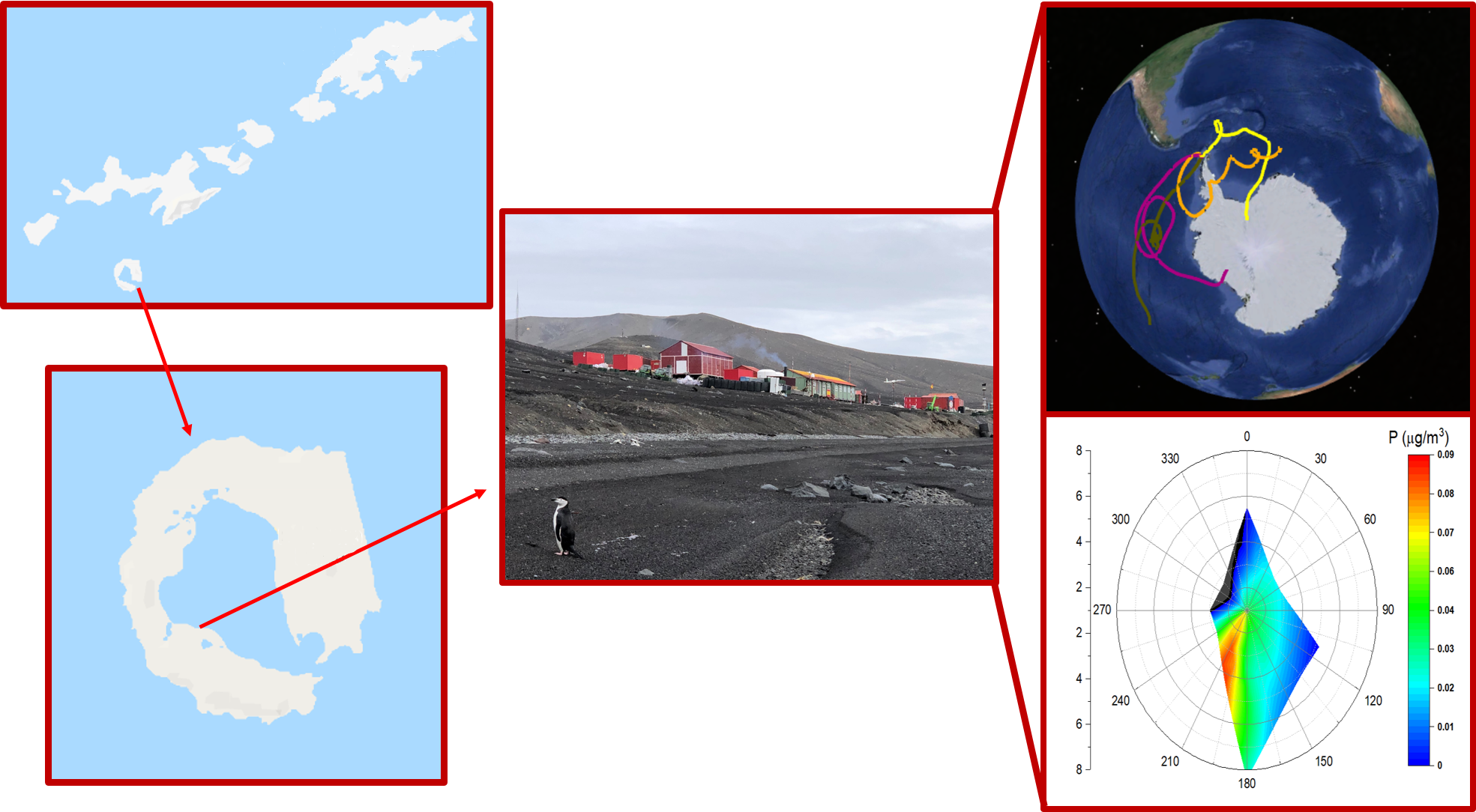
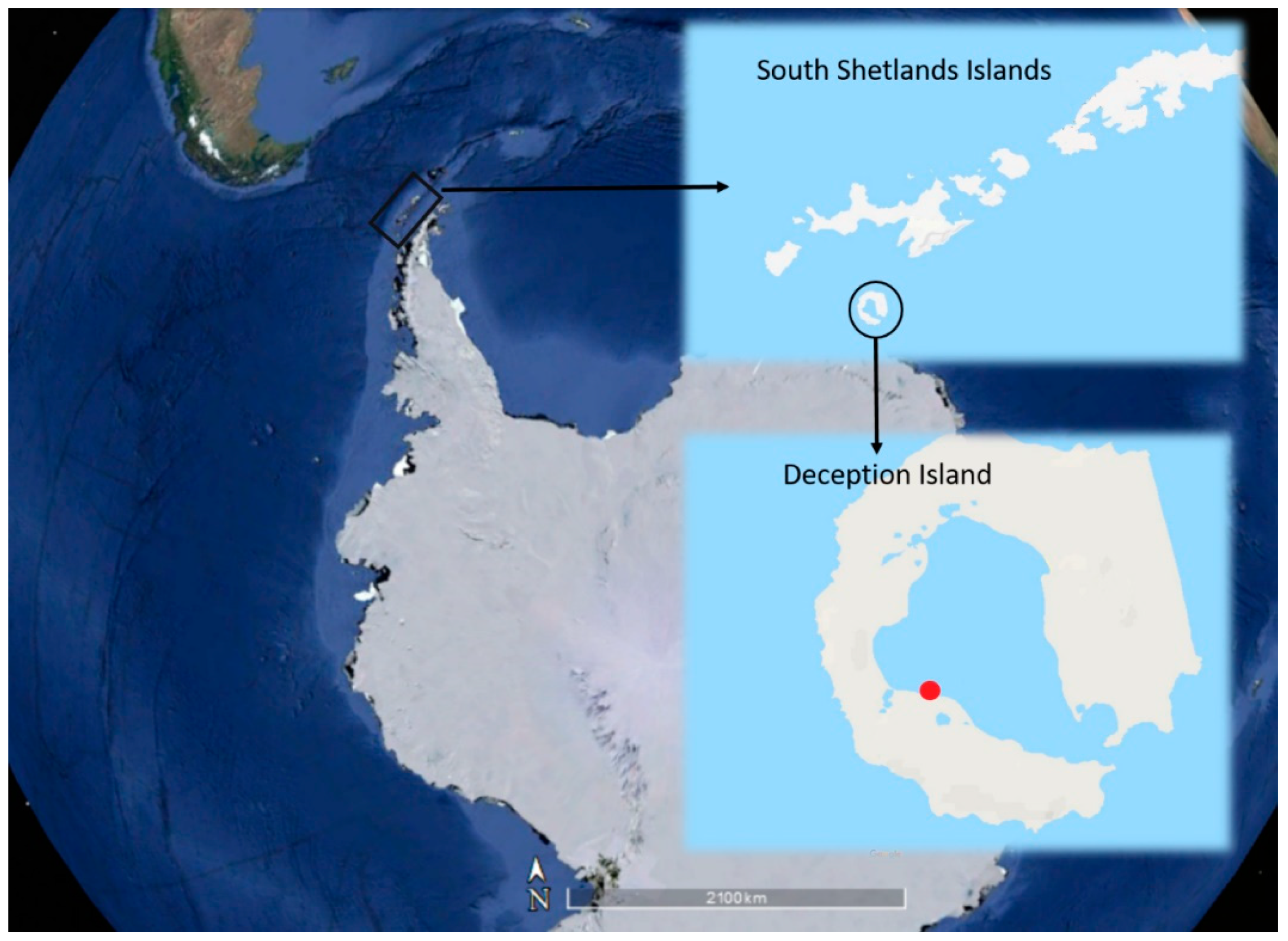
Figure 1.
Map of Deception Island with the location of Gabriel de Castilla Spanish Antarctic Research Station. The red circle point indicates the position of the research base.
Figure 1.
Map of Deception Island with the location of Gabriel de Castilla Spanish Antarctic Research Station. The red circle point indicates the position of the research base.

Figure 2.
Histogram of normal and lognormal statistical distribution for the total particulate material obtained during the 2016–2017 field campaign. Frequency indicates the number of days.
Figure 2.
Histogram of normal and lognormal statistical distribution for the total particulate material obtained during the 2016–2017 field campaign. Frequency indicates the number of days.

Figure 3.
Scatterplot with scores from statistical analysis of the different sampling days by principal component analysis (PCA). (a) represents the whole data set computed as variables. (b) represents the data of the majority elements. (c) represents the data of the trace elements. The green circle, and red and green arrows indicate values that are out of the general behavior.

Figure 4.
Total 10-day air mass backward trajectories at Gabriel de Castilla Station using GDAS1 (Global data assimilation system) dataset.
Figure 4.
Total 10-day air mass backward trajectories at Gabriel de Castilla Station using GDAS1 (Global data assimilation system) dataset.

Figure 5.
(a) Polar contour maps in relation to wind direction and speed for phosphorus (P) and (b) potassium (K) at the Gabriel de Castilla Spanish Research Station (Deception Island).
Figure 5.
(a) Polar contour maps in relation to wind direction and speed for phosphorus (P) and (b) potassium (K) at the Gabriel de Castilla Spanish Research Station (Deception Island).


Table 1.
Particulate matter (PM) statistical summary together with central tendency, variability, and distribution form.
Table 1.
Particulate matter (PM) statistical summary together with central tendency, variability, and distribution form.
| Total Particulate Matter (µg/m3) | |
| Date | PM10 (µg/m3) |
| 28 December 2016 | 6.1 |
| 30 December 2016 | 28.2 |
| 01 January 2017 | 21.7 |
| 07 January 2017 | 8.1 |
| 21 January 2017 | 12.2 |
| 22 January 2017 | 2.9 |
| 23 January 2017 | 9.4 |
| 01 February 2017 | 4.3 |
| 08 February 2017 | 3.8 |
| 14 February 2017 | 2.9 |
| 17 February 2017 | 4.7 |
| 23 February 2017 | 12.1 |
| 24 February 2017 | 19.5 |
| 25 February 2017 | 7.4 |
| 26 February 2017 | 6.0 |
| PM10 Statistical Overview | |
| Number of samples | 15 |
| Average | 9.95 |
| Standard deviation | 7.60 |
| Coefficient of variation | 76.4% |
| Minimum | 2.9 |
| Maximum | 28.2 |
| Range | 25.3 |
| Standard Skewness | 2.1299 |
| Standard Kurtosis | 0.8392 |
Table 2.
P-values obtained for P, K and Cu in PM10 after Kolmogorov–Smirnov test.
| Lognormal | Normal | |
|---|---|---|
| Phosphorus | 0.806278 | 0.0123709 |
| Potassium | 0.735451 | 0.0267816 |
| Copper | 0.288687 | 0.315736 |
© 2020 by the authors. Licensee MDPI, Basel, Switzerland. This article is an open access article distributed under the terms and conditions of the Creative Commons Attribution (CC BY) license (http://creativecommons.org/licenses/by/4.0/).
Share and Cite
MDPI and ACS Style
Marina-Montes, C.; Pérez-Arribas, L.V.; Anzano, J.; Cáceres, J.O. Local and Remote Sources of Airborne Suspended Particulate Matter in the Antarctic Region. Atmosphere 2020, 11, 373. https://0-doi-org.brum.beds.ac.uk/10.3390/atmos11040373
AMA Style
Marina-Montes C, Pérez-Arribas LV, Anzano J, Cáceres JO. Local and Remote Sources of Airborne Suspended Particulate Matter in the Antarctic Region. Atmosphere. 2020; 11(4):373. https://0-doi-org.brum.beds.ac.uk/10.3390/atmos11040373
Chicago/Turabian StyleMarina-Montes, César, Luis Vicente Pérez-Arribas, Jesús Anzano, and Jorge O. Cáceres. 2020. "Local and Remote Sources of Airborne Suspended Particulate Matter in the Antarctic Region" Atmosphere 11, no. 4: 373. https://0-doi-org.brum.beds.ac.uk/10.3390/atmos11040373
Note that from the first issue of 2016, this journal uses article numbers instead of page numbers. See further details here.