Definition and Application of a Protocol for Electronic Nose Field Performance Testing: Example of Odor Monitoring from a Tire Storage Area

Abstract

Odor pollution is nowadays recognized as a serious environmental concern. Italy still lacks a national regulation about odors, but several regions issued specific guidelines and regulations regarding odor emissions management, which combine olfactometric measurements with dispersion modeling for assessing odor impacts and verifying compliance with acceptability criteria. However, in cases of variable or diffuse sources, this approach is sometimes hardly applicable, because odor emission rates can hardly be estimated. In such cases, electronic noses, or more generally, Instrumental Odor Monitoring Systems (IOMS), represent a suitable solution for direct odor measurement. Accordingly, IOMS are explicitly mentioned in the most recent regional regulations as advanced tools for odor impact assessment. In Italy, data from instrumental odor monitoring have started to have regulatory value; thus the need arises to have specific quality programs to ensure and verify the reliability of IOMS outcomes. This paper describes the monitoring by a commercial electronic nose (EOS507F) of odors from an area dedicated to tire storage, a diffuse source with variable emissions over time, for which dispersion modeling is not applicable. The paper proposes also a protocol for IOMS performance testing in the field, to provide experimental data to support technical groups working on standardization both on the national and European level.

1. Introduction

Nowadays, odor pollution is recognized as a serious environmental issue, and odors are subjected to control and regulations in many countries [1,2]. This is also the case for Italy, where odors currently are one of the major causes of complaints from the population to the local authorities.

Indeed, Italy still lacks a national regulation about odors, but several regions, starting with the Region of Lombardy in 2012, have issued specific guidelines and regulations regarding the management and the characterization of odor emissions (Figure 1).

In analogy with other European regulations, all these guidelines are based on the combination of olfactometric measurements and dispersion modeling for the assessment of odor impacts and the verification of compliance with specific acceptability criteria [2].

Dynamic olfactometry, which is the reference method for odor quantification of emissions [3], allows for the measurement of the odor concentration emitted by an odor source, expressed in odor units per cubic meter (ou_E/m³). The odor concentration, combined with the information related to the emitted airflow, geometry, and nature of the emission source, can be used for the evaluation of the so-called odor emission rate (OER), which is expressed in odor units per unit time (i.e., ou_E/s) and is a measure of the odor flux emitted to the atmosphere.

Then, a suitable dispersion model combines OER, topography, and meteorological data to simulate how odor emissions disperse into the atmosphere from the source to the receptor. Several examples can be found in the scientific literature showing how dispersion modeling can successfully be applied for odor impact assessment from simple and complex sources, alone or in combination with other techniques [4,5,6,7].

However, there are several situations in which source characterization and the estimation of a representative OER is extremely complex, making this approach hardly applicable. Such cases include on one hand activities having variable emissions over time. Variable emissions are typical of discontinuous productions, including for instance plants working “on order,” which work just a few hours a day (e.g., asphalts production), or manufacture different products depending on customers’ requests (e.g., pharmaceuticals). On the other hand, despite significant scientific results achieved in the last years in the field of complex source characterization (e.g., [8,9]), there are several diffuse odor sources for which the assessment of a representative air flow, which is needed for the evaluation of the OER, is critical.

In such cases, the use of electronic noses or, more generally, Instrumental Odor Monitoring Systems (IOMS), may be particularly useful because of their capability of directly determining the odor impact at receptors (i.e., sensible neighborhood close to the plant) or at plant fencelines, without necessarily requiring a precise characterization of the odor source [10]. As a matter of fact, electronic noses currently represent the only method available for the continuous monitoring of odors in the field [11]. These are the main reasons underlying their recent development as air quality monitoring tools: in the last 10 years, there has been an increase in the scientific studies involving the use of electronic noses for the continuous detection and characterization of environmental odors [12,13,14,15,16]. Indeed, among the regional guidelines about odor emissions in Italy, the most recent ones, i.e., those of the regions of Piemonte [17], Friuli Venezia Giulia [18], and Emilia Romagna [19], explicitly mention the electronic nose as a method that can be used in addition to or in substitution of dispersion modeling for odor impact assessment purposes.

This is particularly true for the Italian scenario, where odor pollution is the object of growing attention from the Public Administration and the Local Authorities [20]. In Italy, electronic noses are more and more used for the assessment of odor impacts [21,22,23], and there is an increasing number of situations for which the installation of electronic noses is prescribed in the permits of new or existing plants [24].

Based on this recent evolution in the application of electronic noses for odor monitoring in Italy, entailing that data produced by such monitoring instruments are used for regulatory purposes, the need arises to have specific quality programs to ensure the reliability of IOMS outcomes [25]. As a general rule, standards play an important role in developing functional and reliable products for the global marketplace: they typically provide performance criteria that can be used to optimize the reliability and safety of new products [26]. According to this, standardized quality protocols are particularly needed for the instruments’ performance verification [27].

This is the reason why, in recent years, both on the European and national levels, technical groups were constituted to start working on the standardization of procedures relating to the use of electronic noses for environmental odor monitoring [25,28]. Within the European Standardization Committee CEN TC/264 on air quality, a specific working group (WG41) was established in 2014 to draft a standard related to IOMS. The WG41 is composed of experts from different European countries: because of the high national interests regarding this topic, Italy is the most represented country with seven experts actively participating in the WG. The draft standard, which is still in progress, focuses mainly on the validation procedure to be adopted to prove performance claims, consisting in comparing the IOMS output metric with odor assessment metrics obtained with reference methods, such as field inspections [29] and dynamic olfactometry [3].

Meanwhile, in order to cover the specific interests of the Italian legal authorities, in October 2019, the Italian standardization body UNI published a specific technical norm regarding the qualification of IOMS: the UNI 11761:2019 [30]. This norm identifies the technical requirements related to IOMS for the measurement of odors in ambient air and at emissions, with the aim of providing local authorities and end users with an adequate regulatory text, which allows the qualification of extremely different instruments available on the market. Despite its recent publication, the Italian norm is already under revision, in order to include some crucial aspects emerging from the confrontation of the different stakeholders involved: manufacturers, laboratories, end users, environmental protection agencies, and local authorities.

In this context, this paper describes a case study proposing the use of an electronic nose to monitor the odor emissions and assess the related impact from an area dedicated to the storage of tires. Referring to the above-mentioned reasons that limit the applicability of dispersion modeling, this type of source includes both of them: emissions are extremely variable over time due to the continuous handling of tires, but most of all they are hardly quantifiable. For this type of source, it is not possible to define a suitable sampling methodology nor to evaluate a representative value for the OER, as will be described better in the following paragraphs.

For these reasons, this is the perfect situation for the application of an IOMS: the electronic nose represents an excellent solution for the direct assessment of the odor impact on surrounding territories by means of the continuous monitoring of ambient air at the receptor with the purpose of detecting odors related to the tire storage.

Besides focusing on the description of the experimental approach adopted for the electronic nose training and data processing, this paper focuses on the definition and the application of an experimental protocol for the IOMS performance testing. In line with the purposes of the Italian and European technical groups for standardization, the proposed experimental protocol can be applied directly in the field aiming to provide information about the performance of the instrument for the specific application.

The proposed protocol involves the execution of specific field tests, consisting in the analysis of odor samples representative of the emission source and independent from the training set, during the monitoring, in order to test the electronic nose capability of correctly detecting and classifying the odors under investigation. The IOMS performance is assessed in terms of accuracy index and recall.

This research work was carried out with the aim of providing experimental data to support the activity of the technical groups working on standardization, in the definition of a qualification procedure to verify that the IOMS is fit-for-purpose related to the specific application and to provide a methodology to compare the performance of different instruments available on the market. The introduction of such quality protocols represents a crucial step in the process of making electronic noses a widespread and effective environmental odor impact assessment tool.

2. Materials and Methods

2.1. The Electronic Nose Used for the Study

The electronic nose EOS507F used for this study, commercialized by Sacmi s.c., has been developed in collaboration with the Olfactometric Laboratory of the Politecnico di Milano specifically for environmental odor monitoring in an open field and far from the emission source, i.e., at receptors complaining about the presence of malodors (Figure 2) [31].

The electronic nose is equipped with 6 Metal Oxide Semiconductor (MOS) gas sensors, differing in morphology and operating temperature and characterized by high sensitivity, which provides EOS507F effective use for the detection of odors at very low concentrations, typical of the receptor level [32].

The electronic nose is also equipped with specific systems for humidity regulation and realization of reference air (non-odorous air), allowing outdoor use even in the presence of variable weather conditions [31].

2.2. Description of the Selected Case Study

The selected case study is particularly interesting because it describes the possibility of using an electronic nose in a very peculiar situation characterized by complex odor emission sources, for which the application of the most common odor impact assessment method foreseen by local regulations, based on dispersion modeling, is critical.

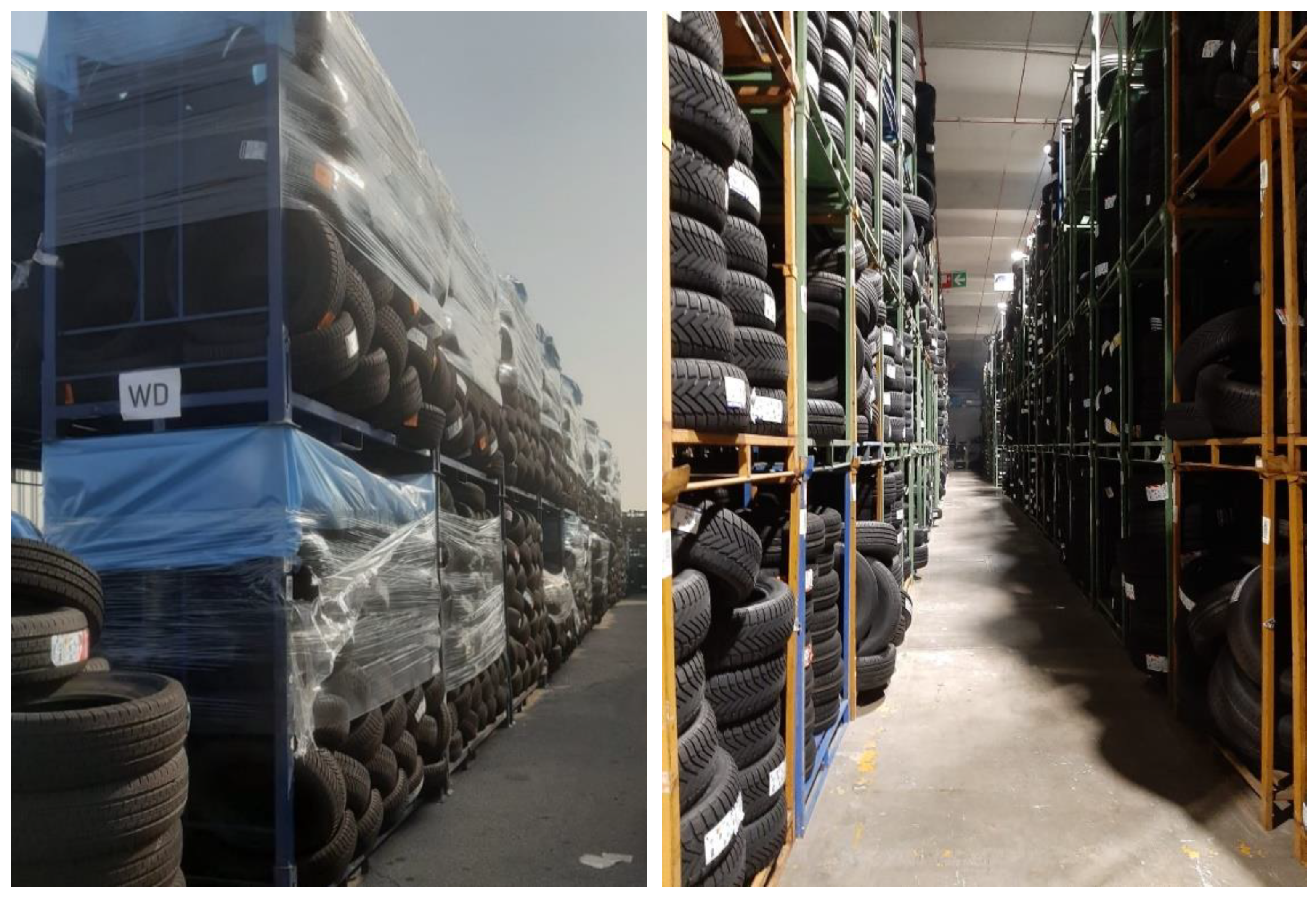
Emissions arising from outdoor tire stacks and tire storage sheds (Figure 3 left and right, respectively), although having a univocal odor character, can hardly be sampled and quantified. In particular, for this type of source, it is not possible to define a suitable sampling methodology nor to evaluate a representative value for the odor emission rate (OER).

Tire storage sheds can be considered as a volume source from which odors are emitted unintentionally from doors and windows. However, characterizing emissions from such sources is challenging, since it is difficult to define a precise air flow and, as a consequence, a representative OER. The most common approach involves the collection of odor samples inside the sheds by means of a depression pump and the estimation of the air flow from openings, assuming that the odor concentration is mixed within the building [33].

Conversely, outdoor tire stacks can be considered as a very particular type of solid passive area source. Two general approaches are usually identified to estimate emission rate values from area sources [34,35,36]:

• Micrometeorological methods: emission rates are measured indirectly through the simultaneous measurements of wind velocities and concentrations across the plume profile downwind of the source [37];
• Chamber methods: emission rates are measured directly by using an enclosure of some sort (typically a wind tunnel or a flux chamber [38]). In this technique, data regarding the concentration of compounds of interest or odor in samples obtained from the device are combined with data regarding the physical dimensions of the device and operating conditions to calculate an emission rate.

Indirect techniques such as micrometeorology do not perturb the emission because of the absence of a sampling device over the emitting surface. However, the measurement methods needed to characterize the emitted plume, involving a large number of samples or high-frequency analyzers, make it impractical for odor assessments [39].

On the other hand, direct methods involving the use of hoods have become very popular for the assessment of odor emissions from area sources. The Odor Emission Rate (OER) is estimated on the basis of the concentration of the samples collected at the outlet of the hood, according to the following Equations [33]:

$$OER=SOER\times A_{em}$$

(1)

$$SOER=\frac{Q_{air}\times c_{od}}{A_{hood}}$$

(2)

where SOER is the Specific Odor Emission Rate (ou_E/m²/s), $A_{em}$ is the area of the emitting surface (m²), $Q_{air}$ is the flowrate of the sweep air (m³/s), $c_{od}$ is the odor concentration (ou_E/m³) of the sample collected at the hood outlet, and $A_{hood}$ is the base area of the hood (m²).

It is important to mention that the SOER obtained this way refers to the sampling conditions; different models have been developed in order to relate the concentration measured at the hood outlet to the effective odor emissions that occur in the open field when the source is exposed to the wind action and which are a function of several different factors [40,41].

However, the applicability of such direct methods is based on the possibility to isolate a portion of the emitting surface, which shall be representative of the emissions of the entire surface. This is obviously not the case for the odor source under investigation (Figure 3, left), which is uneven and thus uncoverable by means of any type of sampling hood and is intrinsically nonhomogeneous. The nonhomogeneity is given by the fact that the tires stored are of hundreds of different types (different manufacturers, models, and sizes), making it impossible to identify a portion of the source that may be representative of the overall emissions.

That is why the application of the techniques for sampling on solid passive area sources—even the most advanced ones—is not applicable in this case.

Another aspect that makes it impossible to apply a dispersion model in this case is related to the high variability of the emission sources over time, due to the continuous handling of tires. This variability constantly alters the emission scenario, especially for the outdoor odor sources, and can hardly be implemented in a dispersion model [10].

For these reasons, the selected study represents a perfect example of a case for which dispersion modeling is not applicable, and thus the electronic nose becomes the best option to assess the odor impact caused by the activity under investigation. This option is also foreseen by the most recent guidelines on odor emissions issued by some Italian regions [17,18,19].

2.3. Electronic Nose Training

The electronic nose training represents the most important phase of the instrumental odor monitoring process [42]. It consists of the creation of the dataset (i.e., the training set—TS) comprising the characteristic “patterns” [43] of the odors that the instrument will be exposed to during the monitoring phase. This database is used by the IOMS as a reference for the classification (i.e., the recognition of the odor quality) of the ambient air that it analyzes during the monitoring phase at the receptor or at the plant fence line.

In general, the first step of the training phase involves a thorough site inspection and the study of the process for the purpose of identifying all potential odor sources of the activity under investigation, which could originate the presence of odors outside the plant, at receptors.

Then, the training involves specific olfactometric campaigns to characterize and quantify those odor emissions and collect samples to be presented to the electronic nose for building the Training Set. This phase is of crucial importance and shall be carried out by experts in the field of odor monitoring in order to identify the relevant odor sources and choose the most suitable strategies for odor sampling.

In this case, two olfactometric campaigns were carried out, involving the collection, by means of a vacuum pump, of samples representative of the characteristic odor of the tires. In this particular situation, the identification of the relevant odor sources turned out to be relatively simple, consisting in the tire storage sheds and the outdoor stacks (Figure 3). Thus, ambient air samples were collected in correspondence with these sources: inside the storage sheds and in the proximity of the outdoor stacks of tires. Nalophan™ bags with a capacity of 7 L, ending with a Teflon™ tube and cap, were used to collect the odorous samples, in compliance with the EN 13725:2003 [3].

10 different samples were collected on two different days in order to partially account for the variability of the source. Indeed, when sampling ambient air, the sample is intrinsically “mixed,” thus being more representative of the overall emissions than a sample collected on only one type of tire, as would be the case if using any sort of enclosure methods. Because the collected samples turned out to be very similar in terms of odor properties and concentration (as shown in Section 3.1), 10 samples were considered sufficient for an instrument training aiming towards the detection of the odors from the tire storage.

The samples representative of the odor emissions from the tire storage were analyzed by dynamic olfactometry, according to the EN 13725:2003 [3], to determine their odor concentration. This step is needed not only to quantify the entity of the odor emissions in terms of odor concentration, but also to evaluate eventual dilution factors to be applied before presenting the samples to the IOMS to build the training set (TS) [21,42].

The dilution with odorless air of the training samples is necessary in order to train the electronic nose with samples having concentration levels similar to those to which the instrument could be exposed during monitoring at the receptor, which are obviously lower than the characteristic concentrations at emission sources. For fenceline monitoring, odor concentrations in the range 30–400 ou_E/m³ can be considered to train the electronic nose [44].

In this specific case, the odor concentrations of the odor samples collected for the electronic nose training were so low (see Section 3.1.) that dilution was not necessary. Thus, the pure odor samples were analyzed by means of the electronic nose in order to build the TS.

The IOMS training involves also the analysis of odorless ambient air samples collected at the monitoring site, when no odor is perceivable by operators, to define the Limit of Detection (LOD), commonly known as “air threshold,” which represents the neutral condition for environmental monitoring (i.e., odor absence). The LOD is assessed per single sensor as the sum of the mean value (C_m) and three times the standard deviation (s_r) of the responses, as reported below [45,46]:

$$\mathrm{LOD}=C_m+3\times s_r$$

(3)

The introduction of the multiplicator term of the standard deviation ($3\times s_r)$ is needed in order to account for the sensor noise. As will be explained further in this paper, the evaluation of the LOD is fundamental to determine the instrument’s sensitivity to the odors under investigation.

For the assessment of the LOD and the creation of the TS, the feature extracted from the sensor signals is the so-called Eos Unit, as described in Dentoni et al. [31].

In this case, two classes were defined to build the TS:

• “Air,” corresponding to the condition of odor absence; and
• “Tire storage,” referring to the characteristic tire odor, which corresponds to the condition of odor presence from the area under investigation.

2.4. IOMS Performance Testing

For the purpose of providing experimental data to support the activity of the technical groups working on standardization, and possibly to guide the revision of the UNI 11761:2019, this paper proposes an experimental testing protocol for IOMS performance verification and presents its application to the specific case of the monitoring of the tire storage area under study.

Given the variety of instruments on the market, multi-purpose or linked to a specific application, the proposed experimental protocol aims to be as general as possible so that it can be applicable to different instruments, differing in hardware and operating principles, designed for various environmental applications. Therefore, the proposed protocol does not concern the instrument hardware but focuses only on its performance.

According to this approach, the instrument is considered as a “black box” by only taking into account the output metrics related to a given stimulus (input), thus ignoring the model that is used to transform the sensor signals into this output.

The proposed testing protocol foresees the verification of some crucial performance requirements of an instrument to be applied for environmental odor monitoring at fenceline or receptors, relevant to the following main functionalities [47]:

• Odor detection: instrument capability of detecting odor presence;
• Odor classification: instrument capability of providing a qualitative characterization of the detected odors;
• Odor quantification: instrument capability of estimating the odor concentration of detected odors.

Although an electronic nose, or more generally an IOMS, cannot be assimilated to an automatic measurement system for continuous monitoring of emissions (AMS), in principle, the approach of the EN 14181:2014 [48] can be re-adapted for defining a procedure for IOMS performance verification [26]. Based on this idea, our research group has been working on the development of a testing procedure, which involves two levels of testing [32,44,45]:

• Level 1 involves tests to be carried out in the laboratory to verify the performance of “multipurpose” instruments by means of suitable synthetic samples with target compounds; and
• Level 2 involves tests to be carried out in the field to verify the performance of the IOMS after training for the specific application and installation at the monitoring site, with the purpose of verifying if the IOMS is or is not fit-for-purpose for the specific monitoring.

The first level of testing involves the analysis of synthetic samples to be carried out in the laboratory under controlled environmental conditions, to provide final users with some preliminary information about the potentialities of the instrument as a monitoring tool, regarding its sensibility towards target compounds and the repeatability of instrument responses [32].

According to the aim of making the testing protocol as general as possible for different environmental applications, the synthetic samples used for laboratory tests should be representative of a wide number of emission types. Based on the scientific literature and our experience in this field, it is possible to state that alcohols, aldehydes, ketones, sulfur compounds, and nitrogen compounds are the most common chemical compound families for odor emissions [32]. Thus, a good strategy for IOMS testing could be the selection of one compound for each of the above-mentioned chemical families.

The first level of testing shall also focus on the verification of the invariability of IOMS responses to variable atmospheric conditions. This aspect is particularly important for outdoor use since abrupt variations of temperature and humidity that may occur during the monitoring represent the main interference on instrument responses associated with the use of electronic noses for the environmental odor monitoring [49,50].

Regarding the first level of testing, which shall be carried out on an instrument before any field application, the whole procedure adopted for sample preparation and analysis, and the results obtained referring to the testing of the EOS507F electronic nose, are reported in previously published works [32,45]. The obtained results proved the instrument capable of detecting the target compounds down to concentrations very close to their odor thresholds and showed an excellent capability of compensating temperature and humidity variations by providing repeatable and accurate odor classifications even under varying conditions of the tested samples.

The second level of testing focuses on the definition of a qualification procedure, which can be carried out in the field, to verify the IOMS performance related to the specific application. This qualification procedure involves the execution of specific field tests after IOMS training and installation at the monitoring site, in the same conditions at which the IOMS will be operating during the monitoring, with the purpose of verifying instrument capability to detect and recognize odors under exam.

In order to test the instrument performance under different atmospheric conditions, field tests should be carried out on different days, characterized by different meteorological conditions.

In the case of IOMS monitoring of plants producing various products or with variable emission sources, the field test should be carried out under different plant operating conditions in order to take into account the intrinsic variability of the emissions.

According to the testing protocol, field tests must be carried out with odor samples collected at odor sources, recognized during the training phase as the main ones responsible for the potential presence of odors outside of the plant under investigation, which have been considered for building the TS. The odor samples to be presented to the instrument during field testing must be independent from the TS in order to ensure a robust estimation of instrument classification performance.

After sampling at emission sources, odor samples must be analyzed by dynamic olfactometry (EN 13725:2003) to determine their odor concentration and dilution factors to obtain odor samples at different concentration levels, within the concentration range considered for the training, to be used for testing.

Besides the definition of dilution factors, the characterization by dynamic olfactometry of odor samples to be presented to the electronic nose allows to investigate the correlation between the instrument outputs and the human perception. Indeed, dynamic olfactometry refers directly to the sensation that the sample causes in a panel of selected people for the assessment of the odor concentration [3]. Thus, the comparison of the electronic nose outcomes during the field tests with odor concentrations measured by dynamic olfactometry is a way of relating the IOMS odor detection performance with the human nose’s detection capability.

Moreover, according to the proposed protocol, the odor samples used in the field to test the electronic nose performance were also given to panelists to obtain a judgment in terms of odor presence or absence. This type of analysis, despite not being based on any standardized methodology, is a simple way to gain immediate and easy information about the correlation between electronic nose outputs and human nose perceptions.

As an alternative and a further improvement, a different field performance testing protocol could be applied, relying on the comparison of the electronic nose outputs with the perception of a selected panel that analyzes the ambient air directly in the field, following an approach similar to the field inspection technique as described in the EN 16841-1:2016 [29]. However, in this specific case in which the source odor concentrations are so low and the expected odor episodes are rare, the application of a field inspection, which is typically highly time- and money-consuming [11,51], was considered not to be sufficiently cost-effective.

Thus, the method involving the field analysis of diluted odor samples was preferred.

The protocol of analysis applied in this case involves the alternate presentation to the IOMS of diluted odor samples at different concentrations to odorless ambient air samples, representative of the neutral condition for the monitoring (i.e., “Air” class), in order to simulate the odor events that might occur during the monitoring at receptors or plant fenceline.

As proposed in previous works [45], the sensitivity towards the odor classes under investigation can be assessed in terms of Lower Detection Limit (LDL). The LDL is easily defined in the case of single sensors: the LDL is the lowest concentration at which the sensor signal produced by a certain substance exceeds the signal relevant to the condition of neutrality. In the case of an IOMS, which is typically a multi-sensor system aiming to produce a response related to odor, the definition of the LDL is less obvious. According to the proposed procedure, the LDL can be established for each odor class under investigation as the lowest concentration at which the IOMS is capable of detecting the presence of an odor sample different from ambient air [45]. As a consequence, the LDL is determined as the lowest concentration level for which at least one sensor of the electronic nose produces a signal that exceeds the signal determined for the LOD (as defined in Section 2.3), meaning that its response is higher than the response to ambient air. Under this assumption, the LDL can be expressed in ou_E/m³ to highlight the relationship to odor.

In the case of a multi-sensor system as an electronic nose, in order to assess the LDL to the odors of interest for the monitoring application, the sensor signals recorded during the field tests of the odor samples at different concentration levels shall be compared with signals corresponding to the LOD determined during the training, as shown in Figure 4.

In a similar way, it is also possible to define the so-called Lower Classification Limit (LCL). The LCL, which can also be expressed in ou_E/m³, can be assessed for each odor class under investigation as the lowest odor concentration at which the IOMS is capable of correctly classifying the odor sample. According to this definition, in those cases in which there is just one odor class to be distinguished from ambient air (as it is in this case), then LDL and LCL coincide.

The determination of the LDL (and LCL) is needed in order to provide final users as well as local authorities with the information about the concentration above which the instrument is capable of recognizing the odor under investigation, which is essential when comparing IOMS detections with citizens’ observations.

In order to quantify the IOMS classification capability, data resulting from the field tests are organized in a confusion matrix (

Table 1. Confusion matrix for the evaluation of the capability of odor detection (TN = true negatives; FN = false negatives; FP = false positives; TP = true positives).

Capability of Odor Detection		IOMS Outcome
		Odor	Air
Odor Class	Odor	TP	FN
	Air	FP	TN

), and the IOMS performance is expressed in terms of accuracy index and recall.

The accuracy index (AI) is defined as the ratio between the number of correctly classified measures and the total measures of samples of known quality and concentration performed:

$$\mathrm{AI}=\frac{\mathrm{TN}+\mathrm{TP}}{\mathrm{TN}+\mathrm{FN}+\mathrm{FP}+\mathrm{TP}}\times 100$$

(4)

The 95% confidence interval (CI) of the accuracy index is estimated as follows [52]:

$$95\% {\mathrm{CI}}_{\mathrm{AI}}=1.96\times \sqrt{\frac{\mathrm{AI}\times \left(1-\mathrm{AI}\right)}{\mathrm{TN}+\mathrm{FN}+\mathrm{FP}+\mathrm{TP}}}$$

(5)

The recall represents the capability of the IOMS to correctly classify samples of a single odor class. Recall and the relevant 95% confidence interval are defined per each class according to the following equations [52]:

$$Recal{l}_{Odor}=\frac{\mathrm{TP}}{\mathrm{FN}+\mathrm{TP}}\times 100$$

(6)

$$95\% {\mathrm{CI}}_{Recal{l}_{Odor}}=1.96\times \sqrt{\frac{Recal{l}_{Odor}\times \left(1-Recal{l}_{Odor}\right)}{FN+TP}}$$

(7)

$$Recal{l}_{Air}=\frac{\mathrm{TN}}{\mathrm{FP}+\mathrm{TN}}\times 100$$

(8)

$$95\% C{I}_{Recal{l}_{Air}}=1.96\times \sqrt{\frac{Recal{l}_{Air}\times \left(1-Recal{l}_{Air}\right)}{\mathrm{FP}+\mathrm{TN}}}$$

(9)

2.5. Continuous Monitoring Phase

After training, the instrument was installed at the northwestern corner of the fenceline of the tire storage area. The choice of the location for the installation of the electronic nose was based on different considerations. First, the proximity to the most critical receptors, i.e., the neighborhood that most frequently complains about the presence of malodors from the monitored plant. Indeed, the nearest and most critical receptor is located very close to the northwestern corner of the plant, and the electronic nose was installed less than 100 m from the first houses.

Other logistic aspects have to be taken into account as well, such as the presence of electricity and the choice of a place that is out of the routes of the vehicles for the tire handling.

The monitoring had a duration of about 45 days, and it was carried out in the period of maximum operation of the tire storage activity.

During the monitoring, the EOS507F performed a continuous analysis of ambient air, with an interruption of the measurements every 30 h for the automatic calibration of the instrument with the internal reference and the restoration of the baseline.

The EOS507F records the signals of the six MOS with a frequency of 1 Hz.

2.6. Odor Impact Assessment

For the classification of the ambient air analyzed continuously by the electronic nose, all the data recorded during the monitoring period were processed by means of the Random Forest classifier, which bases the classification on the construction and validation of an entire forest of random uncorrelated decision trees (variables) [53,54]. In more detail, the Random Forest classifier was applied in order to provide a qualitative characterization of EOS507F detections during the monitoring and assess the frequency with which the instrument classified the analyzed air as “Tire storage” over the monitoring period. The determination of the frequency of the odor detections can be interpreted as a quantitative assessment of the odor impact relevant to the tire storage area at the fenceline, which is considered to be representative of the nearest receptor, located at less than 100 m from the electronic nose installation point.

Concerning the evaluation of the acceptability of the odor impact relevant to an industrial activity, it is possible to refer to the German guideline “GIRL—Geruchsimmision-Richtlinie” dated 13 May 1998 on odor inputs [55]. This guideline establishes an acceptability criterion in terms of “odor hours”, which can be perceived by the neighboring population. The limit of acceptable “odor hours” is fixed at 10% for residential or mixed areas, while this limit is set at 15% for industrial or agricultural areas. The “odor hour” is defined by referring to a specific analysis method called “field inspection,” which was standardized in Europe by the EN16841:2016-Part 1 [29] and represents an hour in which the odor is perceived for more than 10% of the time, therefore for more than 6 minutes. Although the percentage set by this guideline and the definition of odor hours are not directly applicable to the case of IOMS, it is reasonable to refer to the aforementioned guideline, as to date there are no other legislative references and/or acceptability criteria regarding specifically environmental odor monitoring carried out by IOMS.

3. Results

3.1. Odor Concentration of the Training Samples

Table 2. Odor concentrations of the samples collected at the odor sources, used to train the IOMS.

Sample	Odor Concentration (ouE/m3)	Confidence Interval 95% (ouE/m3)
A1	32	14–62
A2	36	16–69
A3	380	170–740
A4	29	13–56
A5	34	15–66
A6	72	32–140
A7	18	8–35
A8	25	11–48
A9	19	8–37
A10	23	10–44

reports the results of the odor concentration measurements of samples collected in correspondence to the emission sources, i.e., inside the tire storage sheds and in the vicinity of the outdoor stacks of tires, which were used for the electronic nose training.

It is possible to highlight that the odor concentration values are very low (Table 2). Nine samples out of 10 are below 80 ou_E/m³, which is the odor concentration value identified by most Italian regional guidelines as the lower limit below which an odor emission shall be considered as negligible. The only exception is represented by sample no. 3, for which a higher odor concentration of 380 ou_E/m³ was measured. The resulting average odor concentration is equal to ca. 40 ou_E/m³, which is a value typical of odorless ambient air.

Considering that the samples were collected in correspondence to the odor sources (i.e., close to tire stacks), based on these numbers, it is possible to state that the odor emissions related to the activity under investigation are not critical from the point of view of the emitted odor concentration.

Nonetheless, the execution of the instrumental odor monitoring is of essential importance in order to objectively quantify the presence of odors at receptors and verify the frequent complaints about the presence of malodors by the close neighborhood.

Given these low odor concentration values, the samples could not be further diluted for the electronic nose training, and thus they were used pure.

The TS data were processed by means of Principal Component Analysis (PCA) with the aim of reducing the dataset dimensionality and obtaining a graphic visualization of the electronic nose discrimination capability between the different odor classes considered for the instrumental odor monitoring.

Figure 5 shows the PCA score plot relevant to the TS: the two classes considered, i.e., “Air” and “Tire storage” are grouped ("clustered") in two different areas of the plot, highlighting the potentiality of the EOS507F to discriminate the tire odor from odorless air.

3.2. IOMS Performance Testing in the Field

This section presents the application of the proposed IOMS testing protocol for the performance verification of the instrument used for the study, i.e., the EOS507F, limiting the description to the results relevant to the second level of testing as described in Section 2.4. Preliminary performance verification tests carried out in the laboratory with synthetic samples, proving that the EOS507F is an instrument capable of providing reliable responses even in presence of variable meteorological conditions and at very low concentrations (i.e., far from the monitored source), have been reported in the work by Eusebio et al. [32].

After IOMS training and installation at the fenceline of the tire storage area, field verification tests were carried out according to the second level of the proposed IOMS testing protocol.

Since field tests are time-consuming, the number of field tests to execute depends on the duration of the monitoring period, the number of odor classes to be monitored, and the amplitude of the concentration range considered for the specific application. Given the short duration of the monitoring period (i.e., 45 days) and the need to analyze samples from only two classes (“Air” and “Tire storage”), it was decided to carry out the field test on two different days.

In order to verify the invariability of the electronic nose classifications under variable atmospheric conditions (i.e., temperature and humidity) in the field (as already mentioned, this capability was already verified in laboratory conditions), the two days selected for the execution of the field tests were characterized by extremely different meteorological conditions. The first day of field testing was sunny and hot (external temperature of ca. 25–26 °C), thus being representative of a condition of high temperature and dry atmospheric conditions. Conversely, the second day was rainy and relatively cold (external temperature of 9–12 °C), thus being representative of lower temperatures and humidity conditions close to saturation.

For the field tests, eight samples representative of the “Tire storage” odor class were collected at the odor emission sources (i.e., inside tire storage sheds and in the proximity of outdoor tire stacks) and analyzed by dynamic olfactometry for the purpose of defining the dilution factors to obtain samples at different concentration levels for IOMS performance testing, and thereby accounting for the relationship between the electronic nose detection capability and human perception.

The resulting odor concentration values of samples used for the EOS507F performance testing are reported in

Table 3. Odor concentration of the odor samples collected for the electronic nose performance testing.

“Tire Storage” Sample	Odor Concentration (ouE/m3)	Confidence Interval 95% (ouE/m3)
B1	30	13–58
B2	36	16–69
B3	50	22–97
B4	40	18–77
B5	60	26–120
B6	20	9–39
B7	60	26–120
B8	25	11–48

.

Additionally, in this case, the measured odor concentration values turned out to be very low, in agreement with the odor concentrations of the samples used for the electronic nose training: all samples had an odor concentration lower than 60 ou_E/m³.

For this reason, only pure samples were analyzed by means of the electronic nose during the field test for performance verification. This of course implies a reduction in the number of tests that could be executed in the field, since the dilution of the samples at higher concentrations to obtain more diluted samples at different concentration levels entails the possibility to multiply the number of measurements that are carried out by the instrument.

Field tests involved also the collection at the fenceline, when no odors could be perceived, of ambient air samples, representative of the “Air” class, which were presented to the IOMS at the beginning of the testing day and between different “Tire storage” samples.

The adopted experimental protocol foresees the alternation of samples representative of the “Air” and “Tire storage” classes to be presented to the IOMS, with the purpose to simulate eventual odor events that might occur during the monitoring.

Table 4. Details of the field tests carried out for performance verification.

	Sample Analyzed	Real Odor Class	Odor Concentration (ouE/m3)	IOMS Classification
First day of testing	C1	Air	-	Air
	B1	Tire storage	30	Tire storage
	C2	Air	-	Air
	B2	Tire storage	36	Tire storage
	C3	Air	-	Air
	B3	Tire storage	50	Tire storage
	C4	Air	-	Air
	B4	Tire storage	40	Tire storage
Second day of testing	C5	Air	-	Air
	B5	Tire storage	20	Air
	B6	Tire storage	60	Tire storage
	C6	Air	-	Air
	B7	Tire storage	60	Tire storage
	C7	Air	-	Air
	B8	Tire storage	25	Air

reports the details of the field tests, thereby indicating whether the electronic nose was capable of correctly classifying the analyzed sample or not. In particular, Table 4 reports the real odor class of samples analyzed, their odor concentration, and the classification provided by the instrument.

The EOS507F correctly classified all samples representative of the “Air” class, and six out of the eight “Tire storage” samples. The two samples belonging to the odor class “Tire storage” that were wrongly classified by the instrument as “Air” had very low odor concentrations (i.e., 20 and 25 ou_E/m³, respectively). These values are so low as to make them practically comparable to odorless ambient air. Indeed, the presence of tire odor in those samples was hardly recognizable even to the human nose; as previously mentioned, the odor samples used for the electronic nose field testing were also analyzed as such by panelists in order to obtain their judgment in terms of odor presence/absence.

The analyses of “Tire odor” samples at different concentrations allowed the assessment of the EOS507F Lower Detection Limit (LDL) [45] towards tire odor, as defined in Section 2.4, which turned out to be equal to 30 ou_E/m³.

As already mentioned, in this case, the LDL of the instrument coincides with its LCL. Indeed, all the samples representative of the tire odor above the concentration of 25 ou_E/m³ were correctly classified by the electronic nose as “Tire storage” samples. These results can be considered as satisfactory, especially in consideration of the fact that the electronic nose is installed at the plant fenceline.

From this example, despite the limited number of analyzed samples, the importance of the determination of the LDL (and LCL) becomes evident: it allows the final user and local authorities to know the concentration above which the instrument is capable of recognizing the odor under investigation. The knowledge of this value is crucial especially in those situations in which the IOMS detections are compared with the observations from the resident population.

The results of the field tests reported in Table 4 were organized in the form of a confusion matrix, as shown in

Table 5. Confusion matrix relevant to the results of the field test.

Capability of Odor Detection		IOMS Outcome
		Tire storage	Air
Odor Class	Tire storage	6	2
	Air	0	7

, in order to quantify EOS507F capability to correctly detect and classify tire odors.

The resulting value for the classification accuracy is 86%, as reported in

Table 6. Accuracy index determined during field tests.

Accuracy Index	95% CI
0.86	±0.18

. Moreover,

Table 7. Recall determined during field tests for odor classes considered.

Odor Class	Recall	95% CI
Tire storage	0.75	±0.30
Air	1	±0

reports the values for the recall, which are 75% and 100% for the “Tire storage” and “Air” odor classes, respectively.

These values can be evaluated as satisfactory for the selected application. As a reference, it is possible to consider the VDI3518-3:2018 “Odour-related measurements with electronic noses and their testing” [47], which, in Section 8.4.3 “Odorant identification (F2)” regarding the electronic nose testing for odorant identification capability, fixes a limit for the proportion of correct identification of 70%. It shall be highlighted that this limit value of 70% from the VDI refers to the identification of odorants in laboratory conditions, which are certainly less critical than field conditions, which makes it the case that the accuracy and recall values obtained in this study can be considered as particularly satisfactory.

Thus, in conclusion, the specific field tests proved that the electronic nose has a good capability of detecting the presence of the characteristic tire odor from the activity of tire storage under investigation, down to odor concentrations of 30 ou_E/m³, and thus that it can be conveniently used for the direct odor impact assessment related to a tire storage area.

3.3. Analysis of the Monitoring Data

The electronic nose data relevant to the monitoring period were processed by application of the Random Forest classifier to provide a qualitative characterization of the analyzed ambient air.

In order to evaluate the possible existence of weather conditions and/or time slots favoring the detection of odor by the electronic nose, the IOMS outcomes were compared punctually with the meteorological conditions.

In more detail, a wind rose relevant to the monitoring period was built by studying the directions of the wind vector by time slots (Figure 6): morning (from 4:00 to 9:00), afternoon (from 10:00 to 15:00), evening (from 16:00 to 21:00) and night (from 22:00 to 03:00). According to the convention adopted, the values reported in Figure 6 refer to the previous 60 min. For example, hour 16 indicates the 60 min from 15:00 to 16:00. Although in meteorological practice wind roses report, by convention, the direction of origin of the wind, in this study the wind rose does not represent the wind direction (i.e., the angle of origin), but rather the wind vector (i.e., the direction towards which the wind blows).

The analysis of the wind rose shows that it was not possible to identify a prevailing wind direction during the monitoring period. This condition is typical of flat areas characterized by very low wind speeds, as is the case of the region where the tire storage area is located, for which a prevailing wind direction is generally not identifiable.

It should be noted that this condition is particularly unfavorable as regards the detection of odors in the vicinity of the plant under examination, in the sense that in such conditions, the probability of detection of odors is maximized, since the dispersion capability of the odor source is very low [56].

However, the study highlighted that the wind blew mostly from south/southeast to north/northwest in afternoons and evenings, thus favoring, in these time slots, the detection of odors from the tire storage by the electronic nose EOS507F, which was installed on the northwestern corner of the plant fenceline.

Indeed,

Table 8. Detail of the “Tire storage” detections by the electronic nose EOS507F during the 45-day monitoring period(S = south; SSE = south-southeast; ESE = east-southeast; E = east; SSW = south-southwest).

“Tire Storage” Detections	Day	Hour	Wind Speed (m/s)	Wind Direction (Origin of Wind)
1	1	16:00–18:00	<1	S/SSE
2	2	14:00–17:00	<1	SSE/ESE
3	20	5:00–9:30	0	-
4	22	8:00–8:30	<1	S/SSW
5	22	20:30–21:45	<1	E
6	23	00:20	<1	E
7	24	10:40–15:25	<1	SSW
8	42	4:00–4:30	<1	SSE

, listing “Tire storage” detections by the EOS507F occurred during the monitoring period, highlights that the electronic nose detected the presence of odors attributable to the tire storage mainly in the afternoon and evening hours, when the wind blew from the south. Only detections 5 and 6 occurred when the wind blew from east to west.

3.4. Quantification of the Odor Impact Related to the Tire Storage Activity

For the purpose of assessing the odor impact relevant to the investigated tire storage area, the EOS507F detections at the fenceline were elaborated and the frequency of detection of the considered classes (i.e., “Air” and “Tire storage”) was assessed.

The electronic nose EOS507F detected the presence of odors attributable to “Tire storage” for the 5% of the total monitoring time. For the remaining time (i.e., 95%), the electronic nose signals never exceeded the Limit of Detection LOD; thus, the EOS507F classified the analyzed ambient air as “Air,” thereby indicating the absence of odors from the monitored plant.

As mentioned in the previous paragraph, the odor episodes occurred mainly in the afternoon and evening hours, characterized, as evidenced by the analysis of the meteorological data, by weather conditions particularly favorable to the detection of odorous emissions from the tire storage area under investigation.

Based on the results obtained, the odor impact relevant to the tire storage area under examination at the fenceline is largely within the limits of acceptability established by the "GIRL—Geruchsimmision-Richtlinie" guideline of 13 May 1998 on odor immissions [55], i.e., 10% of "odor hours" per year that can be perceived by the neighboring population in the case of a residential or mixed zone.

4. Conclusions

This paper has the aim of discussing the advances in odor monitoring with electronic noses in Italy, based on the description of a case study relevant to the monitoring of odors emitted from a tire storage area, by highlighting the potentialities of this technology for the direct assessment of the odor impact, especially in those situations for which approaches based on dispersion modeling are hardly applicable.

After training with samples collected inside the tire storage sheds and in the vicinity of the outdoor stacks of tires, the electronic nose was installed for the monitoring at the fenceline of the tire storage area. The odor impact relevant for the storage area under investigation resulted largely within the limits of the acceptability criteria proposed by the "GIRL—Geruchsimmision-Richtlinie" guideline of 13 May 1998 on odor immissions [54], since the EOS507F detected the presence of odors attributable to the tire storage only for the 5% of the monitoring time.

However, the main objective of the paper is the definition and the application of a specific experimental protocol for the IOMS field performance testing. The applied quality protocol involves the execution of field tests, analyzing dedicated odor samples different from the ones used for the training, to test the electronic nose capability to correctly detect and classify the odors under investigation.

According to the proposed testing protocol, the IOMS capability of correctly detecting and classifying odors was verified in terms of Lower Detection Limit (LDL) and Lower Classification Limit (LCL)—which in this specific case coincide—to the odors under investigation, and of classification accuracy index. The LDL (and LCL) turned out to be equal to 30 ou_E/m³, which is very satisfactory, especially in consideration of the fenceline application. Moreover, the EOS507F capability to discriminate ambient air from “Tire storage” odor was quantified in an 86% accuracy index, thus proving a satisfactory classification performance, referring for instance to the limit value of 70% established by the VDI 3518-3:2018 for electronic nose testing in laboratory conditions.

As a result, the experimental data presented here could support the activity of the technical groups working on standardization, in the definition of a qualification procedure to verify that the IOMS is “fit-for-purpose” related to the specific application, and provide a methodology to compare the performance of different instruments available on the market. Indeed, the monitoring of the tire storage area, representing a relatively simple case study for the electronic nose monitoring, was selected for the purpose of tuning up the experimental protocol, and the results achieved in this study prove the applicability of the proposed testing protocol as an effective method for the IOMS performance verification related to the specific application. However, further investigation should focus on the validation of the proposed testing protocol by considering more complex case studies, involving, for instance, the classification of more odor classes, characterized by similar chemical profiles.

As a conclusion, the proposed procedure could possibly be useful for the purpose of overcoming the skepticism around electronic nose technology that is sometimes manifested by the different stakeholders dealing with the management of odor pollution issues, since the definition and the introduction of common quality protocols represents a crucial step in the process of making electronic noses a widespread and effective environmental odor impact assessment tool.

References

1. Nicell, J.A. Assessment and regulation of odour impacts. Atmos. Environ. 2009, 43, 196–206. [Google Scholar] [CrossRef]
2. Brancher, M.; Griffiths, K.D.; Franco, D.; De Melo Lisboa, H. A review of odour impact criteria in selected countries around the world. Chemosphere 2017, 168, 1531–1570. [Google Scholar] [CrossRef] [PubMed]
3. CEN. EN 13725:2003. Air Quality-Determination of Odour Concentration by Dynamic Olfactometry; CEN: Brussels, Belgium, 2003. [Google Scholar]
4. Sironi, S.; Capelli, L.; Céntola, P.; Del Rosso, R.; Pierucci, S. Odour impact assessment by means of dynamic olfactometry, dispersion modelling and social participation. Atmos. Environ. 2010, 44, 354–360. [Google Scholar] [CrossRef]
5. Capelli, L.; Sironi, S.; Del Rosso, R.; Centola, P.; Rossi, A.; Austeri, C. Odour impact assessment in urban areas: Case study of the city of Terni. Procedia Environ. Sci. 2011, 4, 151–157. [Google Scholar] [CrossRef] [Green Version]
6. Oettl, D.; Kropsch, M.; Mandl, M. Odour assessment in the vicinity of a pig-fatting farm using field inspections (EN 16841-1) and dispersion modelling. Atmos. Environ. 2018, 181, 54–60. [Google Scholar] [CrossRef]
7. Ranzato, L.; Barausse, A.; Mantovani, A.; Pittarello, A.; Benzo, M.; Palmeri, L. A comparison of methods for the assessment of odor impacts on air quality: Field inspection (VDI 3940) and the air dispersion model CALPUFF. Atmos. Environ. 2012, 61, 570–579. [Google Scholar] [CrossRef]
8. Prata, A.A., Jr.; Lucernoni, F.; Santos, J.M.; Capelli, L.; Sironi, S.; Le-Minh, N.; Stuetz, R.M. Mass transfer inside a flux hood for the sampling of gaseous emissions from liquid surfaces—Experimental assessment and emission rate rescaling. Atmos. Environ. 2018, 179, 227–238. [Google Scholar] [CrossRef]
9. Invernizzi, M.; Ilare, J.; Capelli, L.; Sironi, S. Proposal of a method for evaluating odour emissions from refinery storage tanks. Chem. Eng. Trans. 2018, 68, 49–54. [Google Scholar]
10. Capelli, L.; Dentoni, L.; Sironi, S.; Del Rosso, R. The need for electronic noses for environmental odour exposure assessment. Water Sci. Technol. 2014, 69, 135–141. [Google Scholar] [CrossRef] [Green Version]
11. Bax, C.; Sironi, S.; Capelli, L. How can odors be measured? An overview of methods and their applications. Atmosphere 2020, 11, 92. [Google Scholar] [CrossRef] [Green Version]
12. Milan, B.; Bootsma, S.; Bilsen, I. Advances in odour monitoring with E-Noses in the Port of Rotterdam. Chem. Eng. Trans. 2012, 30, 145–150. [Google Scholar]
13. Nicolas, J.; Cerisier, C.; Delva, J.; Romain, A.C. Potential of a network of Electronic Noses to assess the odour annoyance in the environment of a compost facility. Chem. Eng. Trans. 2012, 30, 133–138. [Google Scholar]
14. Deshmukh, S.; Jana, A.; Bhattacharyya, N.; Bandyopadhyay, R.; Pandey, R.A. Quantitative determination of pulp and paper industry emissions and associated odor intensity in methyl mercaptan equivalent using electronic nose. Atmos. Environ. 2014, 82, 401–409. [Google Scholar] [CrossRef]
15. Chirmata, A.; Ichou, I.A.; Page, T. A continuous electronic nose odor monitoring system in the city of Agadir Morocco. J. Environ. Prot. 2015, 6, 54–63. [Google Scholar] [CrossRef] [Green Version]
16. Blanco-Rodríguez, A.; Camara, V.F.; Campo, F.; Becherán, L.; Durán, A.; Vieira, V.D.; De Melo, H.; Garcia-Ramirez, A.R. Development of an electronic nose to characterize odours emitted from different stages in a wastewater treatment plant. Water Res. 2018, 134, 92–100. [Google Scholar] [CrossRef]
17. Regione Piemonte. DGR, n. 13-4554 del 9 Gennaio 2017 “L.R. 43/2000—Linee Guida per la Caratterizzazione e il Contenimento delle Emissioni in Atmosfera Provenienti Dalle Attività ad Impatto Odorigeno”; Regione Piemonte: Torino, Italy, 2017. [Google Scholar]
18. Agenzia Regionale per la Protezione dell’Ambiente Friuli Venezia Giulia (ARPAFVG). LG 44.01/SCE “Valutazione Dell’impatto Odorigeno da Attività Produttive”; ARPA FVG: Palmanova, Italy, 2018. [Google Scholar]
19. Agenzia Regionale per la Protezione dell’Ambiente Emilia Romagna (ARPAE). LG 35/DT “Indirizzo Operative Sull’applicazione Dell’art. 272Bis del D.Lgs.152/2006 e ss.mm”; ARPAE: Bologna, Italy, 2018. [Google Scholar]
20. Sistema Nazionale per la Protezione dell’Ambiente (SNPA). Delibera n. 38/2018: Metodologie per la Valutazione Delle Emissioni Odorigene; Sistema Nazionale per la Protezione dell’Ambiente (SNPA): Rome, Italy, 2018.
21. Sironi, S.; Capelli, L.; Centola, P.; Del Rosso, R.; Il Grande, M. Continuous monitoring of odours from a composting plant using electronic noses. Waste Manag. 2007, 27, 389–397. [Google Scholar] [CrossRef]
22. Giungato, P.; De Gennaro, G.; Barbieri, P.; Briguglio, S.; Amodio, M.; De Gennaro, L.; Lasigna, F. Improving recognition of odors in a waste management plant by using electronic noses with different technologies, gas chromatography–mass spectrometry/olfactometry and dynamic olfactometry. J. Clean. Prod. 2016, 133, 1395–1402. [Google Scholar] [CrossRef]
23. Licen, S.; Barbieri, G.; Fabbris, A.; Briguglio, S.C.; Pillon, A.; Stel, F.; Barbieri, P. Odor Control Map: Self Organizing Map built from electronic nose signals and integrated by different instrumental and sensorial data to obtain an assessment tool for real environmental scenarios. Sens. Actuators B Chem. 2018, 263, 476–485. [Google Scholar] [CrossRef]
24. Cangialosi, F.; Intini, G.; Colucci, D. On line monitoring of odour nuisance at a sanitary landfill for non-hazardous waste. Chem. Eng. Trans. 2018, 68, 127–132. [Google Scholar]
25. Cipriano, D.; Capelli, L. Evolution of electronic noses form research objects to engineered environmental odour monitoring systems: A review of standardization approaches. Biosensors 2019, 9, 75. [Google Scholar] [CrossRef] [Green Version]
26. Nagle, H.T.; Schiffman, S.S. Electronic Taste and Smell: The Case for Performance Standards [Point of View]. Proc. IEEE 2018, 106, 1471–1478. [Google Scholar] [CrossRef]
27. Cipriano, D. Application of EN14181 and EN15267 to electronic noses: Challenge or provocation? Chem. Eng. Trans. 2018, 68, 139–144. [Google Scholar]
28. Romain, A.C.; Capelli, L.; Guillot, J.M. Instrumental odour monitoring: Actions for a new European Standard. In Proceedings of the 2017 ISOCS/IEEE International Symposium on Olfaction and Electronic Nose (ISOEN 2017), Montreal, QC, Canada, 28–31 May 2017; IEEE Service Center: Piscataway, NJ, USA, 2017. [Google Scholar]
29. CEN. EN 16481-1:2016. Ambient Air-Determination of Odour in Ambient Air by Using Field Inspection-Part 1: Grid Method; CEN: Brussels, Belgium, 2016. [Google Scholar]
30. UNI. UNI 11761:2019. Emissioni e Qualità Dell’aria—Determinazione Degli Odori Tramite IOMS (Instrumental Odour Monitoring Systems); UNI: Milano, Italy, 2019. [Google Scholar]
31. Dentoni, L.; Capelli, L.; Sironi, S.; Del Rosso, R.; Zanetti, S.; Della Torre, M. Development of an Electronic Nose for Environmental Odour Monitoring. Sensors 2012, 12, 14363–14381. [Google Scholar] [CrossRef] [Green Version]
32. Eusebio, L.; Capelli, L.; Sironi, S. Electronic Nose Testing Procedure for the Definition of Minimum Performance Requirements for Environmental Odor Monitoring. Sensors 2016, 16, 1548. [Google Scholar] [CrossRef] [Green Version]
33. Capelli, L.; Sironi, S.; Del Rosso, R. Odor sampling: Techniques and strategies for the estimation of Odor Emission Rates from different source types. Sensors 2013, 13, 938–955. [Google Scholar] [CrossRef] [Green Version]
34. Laville, P.; Jambert, C.; Cellier, P.; Delmas, R. Nitrous oxide fluxes from a fertilised maize crop using micrometeorological and chamber methods. Agric. For. Meteorol. 1999, 96, 19–38. [Google Scholar] [CrossRef]
35. Shah, S.B.; Westerman, P.W.; Arogo, J. Measuring ammonia concentrations and emissions from agricultural land and liquid surfaces: A review. J. Air Waste Manag. 2006, 56, 945–960. [Google Scholar] [CrossRef] [Green Version]
36. Mønster, J.; Kjeldsen, P.; Scheutz, C. Methodologies for measuring fugitive methane emissions from landfills–A review. Waste Manag. 2019, 87, 835–859. [Google Scholar] [CrossRef]
37. Li, X.; Wang, T.; Sattayatewa, C.; Venkatesan, D.; Noll, K.E.; Pagilla, K.R.; Moschandreas, D.J. Odor emission rate estimation of indoor industrial sources using a modified inverse modeling method. J. Air Waste Manag. 2011, 61, 872–881. [Google Scholar] [CrossRef]
38. Hudson, N.; Ayoko, G.A. Comparison of emission rate values for odour and odorous chemicals derived from two sampling devices. Atmos. Environ. 2009, 43, 3175–3181. [Google Scholar] [CrossRef] [Green Version]
39. Hudson, N.; Ayoko, G.A. Odour sampling. 2. Comparison of physical and aerodynamic characteristics of sampling devices: A review. Bioresour. Technol. 2008, 99, 3993–4007. [Google Scholar] [CrossRef] [Green Version]
40. Lucernoni, F.; Capelli, L.; Busini, V.; Sironi, S. A model to relate wind tunnel measurements to open field odorant emissions from liquid area sources. Atmos. Environ. 2017, 157, 10–17. [Google Scholar] [CrossRef]
41. Prata, A.A., Jr.; Santos, J.M.; Timchenko, V.; Stuetz, R.M. A critical review on liquid-gas mass transfer models for estimating gaseous emissions from passive liquid surfaces in wastewater treatment plants. Water Res. 2018, 130, 388–406. [Google Scholar] [CrossRef]
42. Capelli, L.; Sironi, S.; Céntola, P.; Del Rosso, R.; Il Grande, M. Electronic noses for the continuous monitoring of odours from a wastewater treatment plant at specific receptors: Focus on training methods. Sens. Actuators B Chem. 2008, 131, 53–62. [Google Scholar] [CrossRef]
43. Romero-Flores, A.; McConnell, L.L.; Hapeman, C.J.; Ramirez, M.; Torrents, A. Evaluation of an electronic nose for odorant and process monitoring of alkaline-stabilized biosolids production. Chemosphere 2017, 186, 151–159. [Google Scholar] [CrossRef] [PubMed]
44. Bax, C.; Li Voti, M.; Sironi, S.; Capelli, L. Application and performance verification of electronic noses for landfill odour monitoring. In Proceedings of the Sardinia 2019, Santa Margherita di Pula (Cagliari), Italy, 30 September–4 October 2019; CISA Publisher: Padova, Italy, 2019. ISBN 9788862650144. ISSN 2282-0027. [Google Scholar]
45. Li Voti, M.; Bax, C.; Marzocchi, M.; Sironi, S.; Capelli, L. Testing Procedure for Performance Evaluation of Electronic Noses for Environmental Odour Monitoring. CEt 2018, 68, 277–282. [Google Scholar]
46. Devore, J.L. Probability and Statistics for Engineering and the Science, 8th ed.; Cengage Learning: Boston, MA, USA, 2011. [Google Scholar]
47. VDI. VDI 3518-3:2018. Multigas Sensors—Odour Related Measurements with Electronic Noses and Their Testing; Beuth Verlag: Berlin, Germany, 2018. [Google Scholar]
48. CEN. EN 14181:2014 Stationary Source Emissions—Quality Assurance of Automated Measuring Systems; Comitée Européen de Normalisation: Brussels, Belgium, 2014. [Google Scholar]
49. Liang, Z.; Tian, F.; Yang, S.X.; Zhang, C.; Sun, H.; Liu, T. Study on interference suppression algortithms for electronic noses: A review. Sensors 2018, 18, 1179. [Google Scholar] [CrossRef] [PubMed] [Green Version]
50. Valleis, S.; Gracia, I.; Pizurovà, N.; Figueras, E.; Cechal, J.; Hubalek, J.; Canè, C. Gas sensitive ZnO structures with reduced humidity-interference. Sens. Actuators B Chem. 2019, 301, 127054. [Google Scholar] [CrossRef]
51. Conti, C.; Guarino, M.; Baenetti, J. Measurements techniques and models to assess odor annoyance: A review. Environ. Int. 2020, 134, 105261. [Google Scholar] [CrossRef]
52. Webber, W. Approximate recall confidence intervals. arXiv 2013, arXiv:1202.2880v4. [Google Scholar] [CrossRef] [Green Version]
53. Breiman, L. Random Forest. Mach. Learn. 2001, 45, 5–32. [Google Scholar] [CrossRef] [Green Version]
54. Liaw, A.; Wiener, M. Classification and Regression by RandomForest. R News 2002, 2/3, 18–22. [Google Scholar]
55. LAI (Länderausschuss für Immissionsschutz): Geruchsimmissions—Richtlinie: GIRL—Odour Emissions Guidelines); Ministry of Environment, Environmental Planning, and Agriculture of the State Nordrhein-Westfalen: Berlin, Germany, 1998.
56. Choi, W.; Winer, A.M.; Paulson, S.E. Factors controlling pollutant plume length downwind of majoer roadways in nocturnal surface inversion. Atmos. Chem. Phys. 2014, 14, 6925–6940. [Google Scholar] [CrossRef] [Green Version]
Figure 1. Italian regions having a guideline/regulation on odor emissions: Lombardy (1), Autonomous Province of Trento (2), Piemonte (3), Puglia (4), Friuli Venezia Giulia (5), Emilia Romagna (6).
Atmosphere 11 00426 g001
Figure 2. The electronic nose EOS507F used for the study.
Atmosphere 11 00426 g002
Figure 3. Example of outdoor stack of tires (left) and interior of a storage shed (right).
Atmosphere 11 00426 g003
Figure 4. Assessment of the Lower Detection Limit (LDL) during field tests.
Atmosphere 11 00426 g004
Figure 5. Principal component analysis (PCA) score plot relevant to the Training set.
Atmosphere 11 00426 g005
Figure 6. Wind roses per time slots relevant to the monitoring period.
Atmosphere 11 00426 g006