Scale-Dependent Turbulent Dynamics and Phase-Space Behavior of the Stable Atmospheric Boundary Layer

Abstract

The structure of turbulent dynamics in a stable atmospheric boundary layer was studied by means of a phase-space description. Data from the CASES-99 experiment, decomposed in local modes (with increasing time scale) using empirical mode decomposition, were analyzed in order to extract the proper time lag and the embedding dimension of the phase-space manifold, and subsequently to estimate their scale-dependent correlation dimension. Results show that the dynamics are low-dimensional and anisotropic for a large scale, where the flow is dominated by the bulk motion. Then, they become progressively more high-dimensional while transiting into the inertial sub-range. Finally, they reach three-dimensionality in the range of scales compatible with the center of the inertial sub-range, where the phase-space-filling turbulent fluctuations dominate the dynamics.

1. Introduction

The atmospheric boundary layer (ABL) connects the the lowest layer of the Earth’s atmosphere near the surface to the rest of the free atmosphere (troposphere). Its dynamics are fundamental for the transport and exchange of moisture, heat and momentum with the underlying surface [1,2]. The ABL is characterized by almost continuous variations of thickness. This is particularly true over land, in which case it can reach a thickness of the order of $d\approx 100$ m during the night and $d\approx 2000$–3000 m or even more during the day. Within the ABL dynamics, all physical quantities related with the flow (e.g., velocity, temperature, moisture and density) are characterized by rapid and large amplitude turbulent fluctuations, due to strong vertical mixing and the interplay of waves and turbulent motions [3,4,5]. Among other processes, the advection of warm air over a cooler surface is the principal responsible for the formation of the stable boundary layer (SBL) [1,6,7]. Its formation is mainly related to the radiative cooling of the ground occurring during nighttime conditions under relatively clear skies. The net radiative cooling of the ground surface induces a vertical temperature gradient, associated with a heat transfer from the ABL to the cooler surface, and this heat loss cools the air with the formation of a stable stratified inversion layer. Several studies have examined the turbulent behavior in SBL, showing that its structure can be extremely complex and characterized by multiscale fluctuations in the inertial sub-range [8,9,10,11]. Studies of the mesoscale range (sub-hourly to sub-daily time scales) [12,13,14] suggested the existence of a universal cascade mechanism associated with the energy transfer between synoptic motions and turbulent microscales in the atmospheric boundary layer. Empirical evidence was provided that mesoscale phenomena own a certain degree of universality and share features with the homogeneous, fully developed turbulence. However, these works were performed in order to understand the similarities between different scales in terms of intermittency and cascade models, without exploring the structure and the dynamical properties related to the phase space, or the isotropy–anisotropy dichotomy. Indeed, at large scales, usually characterized by low wind-speed episodes [15,16,17], but also in the inertial sub-range, the SBL turbulent fluctuations can be anisotropic, characterized by quasi two-dimensional structure of the flow. Such behavior has been marked as a distinctive feature of the SBL dynamics. However, some studies indicate that even in strongly anisotropic flows, a sort of recovery of isotropy may exist at smaller scales [18,19,20]. Large eddy simulations have shown that isotropy recovery is a "genuine feature" of the inertial sub-range [21,22]. The statistical properties of homogeneous and isotropic turbulence are usually characterized by means of energy spectral density and by the anomalous scaling of the structure functions of the field increments, e.g., ${\mathcal{S}}_q\propto {\ell }^{\zeta \left(q\right)}$ [23,24,25,26], correlations [27,28,29,30]; or in terms of multifractality from the analysis of the so called multifractal spectrum $f\left(\alpha \right)$ [31,32,33,34,35,36]. However, it is often difficult to clearly disentangle the turbulent fluctuations from the possible superposed large-scale motions, so that the genuine features of the cascade may be covered in the data. In this work, the phase-space of the turbulent velocity fluctuations is reconstructed at different scales, providing information on the dimensionality of the dynamics through the correlation dimensions [37]. It is shown that a marked transition between inertial sub-range turbulence and large-scale features is present, for the first time, in terms of dimensionality of the phase-space manifold. Moreover, observations suggest a possible restoring of isotropy when approaching smaller scales.

2. The CASES-99 Data-Set

In order to characterize the dynamical properties and the phase-space manifold of stable boundary layer turbulence, data from the the CASES-99 experiment has been investigated [38,39]. The experiment has been performed from 01/10/1999 to 31/10/1999 in Kansas, USA (${37.6}^{\circ }$ N, ${96.7}^{\circ }$ E), on a relatively homogeneous and flat experimental area, making it an ideal site for atmospheric boundary-layer study above a homogeneous terrain. During the measurements, horizontal and vertical observations of turbulent velocity components have been performed with temporal resolution $\Delta t=0.05$ s. Accordingly to the standard dynamic stability indicator $\Pi$ [10,40], all the CASES-99 nights can be classified into three categories: turbulent nights, intermittent nights and radiative nights [41]. Here we made use of measurements taken on October 15, 16, and 17, between 00:00 and 06:00, when the SBL was categorized as turbulent. Preliminary analysis shows that the friction velocity for all three samples was similar, $u^{\ast }=\{0.49,0.45,0.59\}$ m s${}^{-1}$, while different net radiation $Q_{\mathrm{net}}=\{-73,-58,-31.2\}$, as well as sensible and latent heat fluxes $H=\{-45.6,-13.8,-5.7\}$ W m${}^{-2}$ and $L_{\mathrm{v}}E=\{5.7,9.2,12.5\}$ W m${}^{-2}$ were observed. After selection, each velocity component has been further partitioned in three sub-intervals of 2 h, which were analyzed individually in order to check for variations in the nighttime SBL dynamics.

3. Empirical Mode Decomposition of SBL Turbulent Fluctuations

Within the empirical mode decomposition (EMD) framework [42,43], the three components of a velocity field $U\equiv \left[u\left(t\right),v\left(t\right),w\left(t\right)\right]$ can be decomposed each into a finite number n of oscillating basis functions, resulting in the intrinsic mode functions (IMFs) $X_j\equiv \left[{\varphi }_j\left(t\right),{\psi }_j\left(t\right),{\theta }_j\left(t\right)\right]$, and additive residuals $R\equiv [r_{\varphi }\left(t\right)$, $r_{\psi }\left(t\right)$, $r_{\theta }\left(t\right)]$ describing the mean trend, so that:

$$U_i\left(t\right)=\sum _{j=1}^n{X}_{i,j}\left(t\right)+R_i\left(t\right),$$

(1)

where $i\doteq \{u,v,w\}$ or $\{{\varphi }_j,{\psi }_j,{\theta }_j\}$. The decomposition algorithm, called the “sifting process,” is based on the local properties of time series [42], thereby allowing one to characterize non-stationary and nonlinear processes thanks to its intrinsic adaptive nature. Here, the 3-thresholds stoppage criterion has been used for interrupting the sifting procedure. This choice has been adopted in order to guarantee globally small fluctuations in the mean, while taking into account locally large variations [43]. The values for the three parameters used in this work are: $\delta =0.05$, ${\xi }_1=0.05$ and ${\xi }_2=10{\xi }_1$, in accordance with their typical values [43]. Moreover, by means of a Hilbert transform, each IMF is modulated both in amplitude and phase, $X_{i,j}\left(t\right)=A_{i,j}\left(t\right)cos\left[{\Phi }_{i,j}\left(t\right)\right]$ being defined by their instantaneous amplitudes and phases [42]. The instantaneous frequency directly comes out as ${\omega }_{i,j}={2\pi }^{-1}d{\Phi }_{i,j}\left(t\right)/dt$, and the mean period ${\tau }_{i,j}={\langle {\omega }_{i,j}\rangle }_t^{-1}$, with ${\langle ·\rangle }_t$ representing time average [42].

When the EMD is applied on turbulent fields; fractal or multifractal processes; and random walks, it intrinsically acts as a dyadic filter bank [44,45,46,47], where each IMF captures a narrow band in frequency space, and the superposition of their Fourier spectra behaves as a power-law $M_{\psi }\left(\omega \right)\equiv \mathrm{Max}\left[\widehat{\psi }\left(\omega \right)\right]\sim {\omega }^{-\beta }$ [14,48,49,50].

The EMD has been applied to the three velocity components of the data-set described above. The resulting IMFs give a complete decomposition of the signal in proper modes, which will be used for the analysis. A simple significance test [44] comparing the energy of the j-th IMFs and a theoretical spread function of white noise, computed for different confidence levels, allows one to distinguish between purely noisy and physical meaningful oscillations [44]. Said test has been performed on all samples used in this work. All IMFs were statistically significant above the 99% confidence level.

Using as an example one velocity component from one of the extracted CASES-99 velocity samples, in Figure 1 we observe that IMFs $2\le j<10$ are sufficient to capture the turbulent cascade process, characterizing the inertial sub-range, and $M_{\psi }\left(\omega \right)\sim {\omega }^{-1.61\pm 0.01}$ for $\omega \in [5\times {10}^{-2},{10}^{0.5}]$ Hz, compatible with the standard Kolmogorov turbulent spectrum [51]. Similar results have been obtained for all components of all samples (not shown).

Since each IMF describes a well defined spectral band, it is possible to associate it to a characteristic timescale, or period, ${\tau }_j$. Figure 2 shows that the calculated periods are similar for all components $X_{i,j}$ and for all samples, and are well ordered so that smaller j corresponds to smaller time-scale, according to a roughly exponential relation (dashed lines).

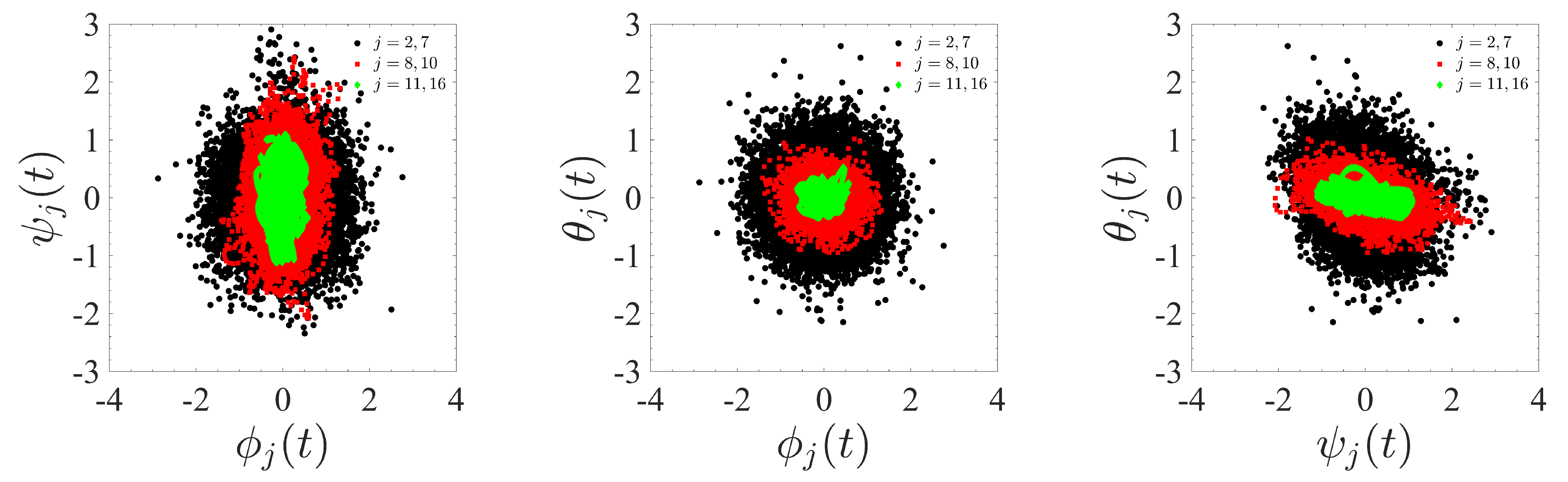
4. Phase-Space Reconstruction and Time Delay of Local SBL Fluctuations

According to Takens theorem, the dynamics of a chaotic system can be reconstructed from a sequence of observations of its state, by embedding a time-delayed version of the original observations, a procedure that preserves geometrical invariants, such as the box-counting dimension of the chaotic attractor [52]. Given a local d-dimensional state vector $X_j\equiv [{\varphi }_j\left(t\right),{\psi }_j\left(t\right),{\theta }_j\left(t\right)]$, which evolves according to a deterministic dynamics, and whose component $X_i$ has been extracted via the EMD decomposition, it is possible to reconstruct the higher dimensional dynamics by using time-delayed versions of the observed quantity $X_{i,j}(t+\ell \Delta t)=X_{i,j}(\ell \Delta t)$ as coordinates for the phase space. This requires the selection of appropriate time delay ℓ [53] and embedding dimension m [54,55]. The embedding dimension represents the minimum dimension of the space in which one can reconstruct a "phase portrait" starting from observations, in which the trajectory does not cross itself. In some cases, the attractor of a dynamical system can present lower dimensionality than the embedding space. In order to perform the phase-space reconstruction briefly described above, we have used the CASES-99 velocity data as follows.

First, the time delay ℓ has been evaluated via the multivariate average mutual information (MI) $I[X_j\left(t\right),X_j(t+\ell )]={\sum }_{a,b}{p}_{a,b}(\ell )log\left(p_{a,b}(\ell )/p_a{p}_b\right)$ (where $p_a$, $p_b$, and $p_{a,b}(\ell )$ are the marginal and joint PDFs of the components of $X_j$) between the original time series and the same time series shifted by the time delay ℓ, averaged over all the data dimensions. For each sample and for each component, the time delay has been selected as to minimize the mutual information [56,57].

Secondly, the optimal embedding dimension m has been evaluated via the false nearest neighbor method (FNN) [55,58], by defining the squared Euclidean distance $Z_{md}^2$, between the components of $X_j$ and its r-th nearest neighbor $X_j^{\left(r\right)}$, in an m-dimensional phase-space, and then extending to an $m+1$-dimensional phase-space, with $1\le d\le 3$:

$$\begin{array}{ccc}\hfill Z_{md}^2& =& \sum _{i=1}^d\sum _{k=0}^{m-1}{\left[X_i(t+k\ell )-X_i^{\left(r\right)}(t+k\ell )\right]}^2\hfill \end{array}$$

(2)

$$\begin{array}{ccc}\hfill Z_{(m+1)d}^2& =& Z_{md}^2+\sum _{i=1}^d{\left[X_i(t+m\ell )-X_i^{\left(r\right)}(t+m\ell )\right]}^2.\hfill \end{array}$$

(3)

If the distance Z does not exceed a selected threshold $Z_{tol}\Delta t^{-1}=15$, $Z<Z_{tol}$, then the embedding procedure leaves the shape of the attractor unchanged, and the points are defined as true neighbors. In that case, the embedding dimension m is selected. On the other hand, if $Z>Z_{tol}$, these points are defined false neighbors, the embedding dimension m is too small to completely unfold the attractor, and the data need to be embedded further (i.e., $m+1$).

Additionally, a secondary step requires that the distance of the nearest neighbor, when embedded into the next higher dimension ($m+1$), should be smaller than a second threshold; say, $A_{tol}\Delta t^{-1}=5$, $Z_{m+1}<A_{tol}$. The optimal embedding dimension m is selected when the percentage of FNN vanishes. Multiplying this dimension m by the number of components of data-set d, provides the true estimate of dimensionality [59]. The procedure is then repeated decreasing the data dimensionality to $d=2$ and then to $d=1$, in order to explore the appropriate embedding dimension. Figure 3 shows the results of the FNN analysis for the components $X_{1,j}$, $X_{2,j}$ and $X_{3,j}$ respectively, of the state vector $X_j$, corresponding to a space $d=1$. All curves relative to IMFs liyng in the inertial sub-range ($2\le j<10$, full symbols) reach a percentage of FNN $=0$ for an embedding dimension $m=3$, corresponding to a dimensionality $md=3$. On the other hand, for IMFs related to large-scale flow ($j\ge 10$, open symbols) the embedding dimension is $m=2$ or $md=2$. Finally, the two largest-scale IMFs drop to a percentage of FNN $=0$ for $m=1$ ($md=1$) for all samples. The same results are obtained for all other samples analyzed in this work. Results of the FNN analysis thus suggest a different dimensionality for the different spectral regions of the atmospheric velocity fluctuations.

Table 1. Time delay ℓ and embedding dimension m for different possible choices of data dimension d and components for the IMF with $j=5$, $X_5\equiv \left[{\varphi }_5\left(t\right),{\psi }_5\left(t\right),{\theta }_5\left(t\right)\right]$, obtained from the SBL sub-sample dated $15/10/99$$02:00\to 04:00$.

SBL $\mathit{j}=5$	d	$\mathit{\ell }\Delta \mathit{t}$[s]	m	$\mathit{dm}$
${\varphi }_5$	1	0.35	3	3
${\psi }_5$	1	0.40	3	3
${\theta }_5$	1	0.35	3	3
${\varphi }_5,{\psi }_5$	2	0.38	2	4
${\varphi }_5,{\theta }_5$	2	0.35	2	4
${\psi }_5,{\theta }_5$	2	0.38	2	4
${\varphi }_5,{\psi }_5,{\theta }_5$	3	0.37	1	3

collects the results of the preliminary analysis: the time lags ℓ, as obtained via the MI; the embedding dimension m; and the total dimensionality $dm$, for different choices of the state vector dimension $d=1,2,3$. Values in the Table refer to $X_5\equiv \left[{\varphi }_5\left(t\right),{\psi }_5\left(t\right),{\theta }_5\left(t\right)\right]$ (central scale of the inertial sub-range; see Figure 1) for the sample dated $15/10/99$$02:00\to 04:00$. For the case $d=1$ (i.e., when using single-component velocity time series), the estimate of the true dimensionality gives $m=3$ or $dm=3$, indicating that each one-dimensional series must be embedded twice in order to describe the phase space. Similarly, setting $d=3$ (i.e., the full three-dimensional vector is used) results in $m=1$ ($md=3$), meaning that the three-dimensional state vector $X_j$ allows for the description of the full phase space and does not need further embedding. Finally, for the various possible combinations of two-dimensional time series ($d=2$), the estimate of the true dimensionality gives $m=2$, resulting in $md=4$, necessary to describe a three-dimensional dynamics using two-dimensional vectors.

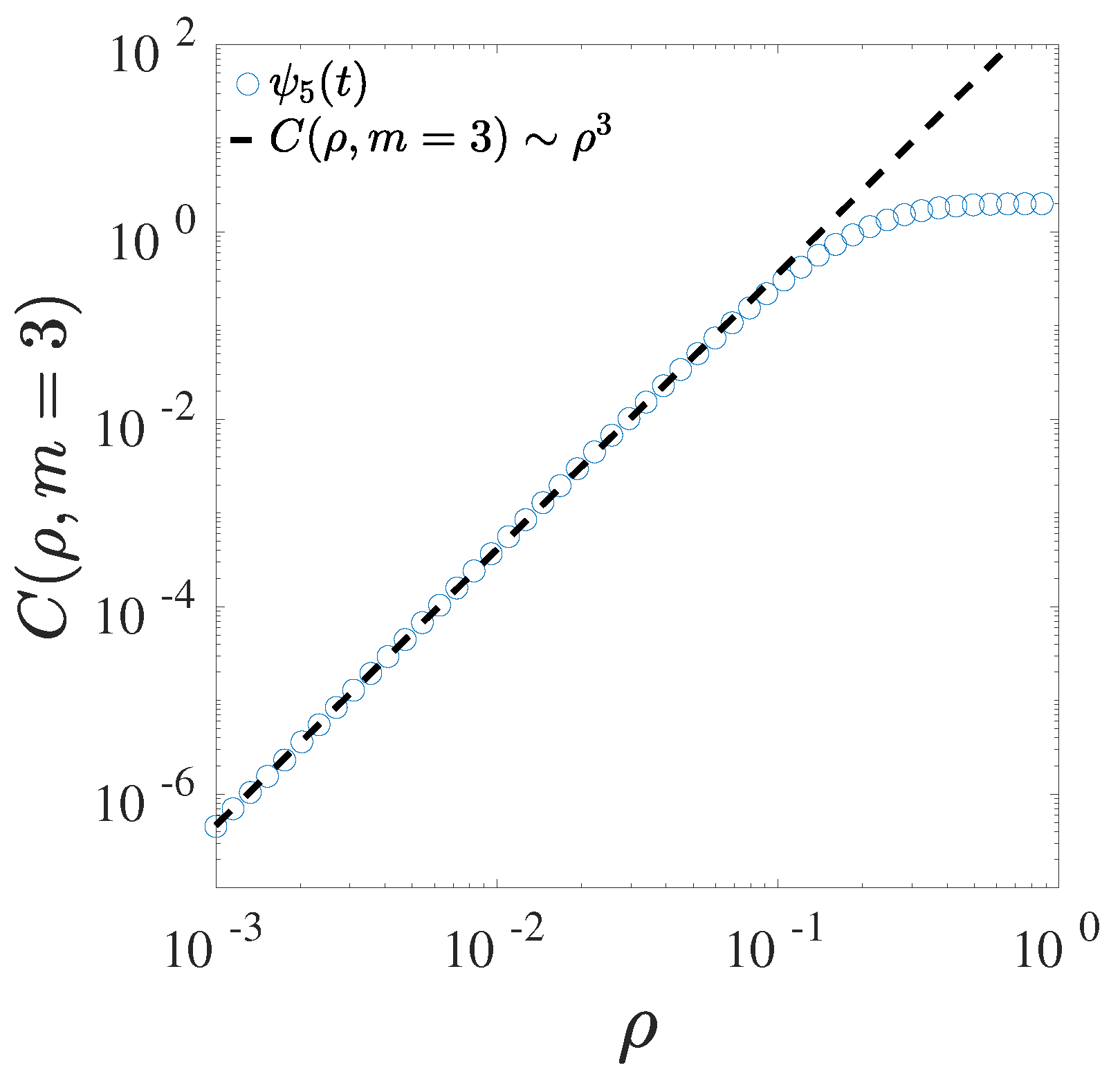
5. Local Correlation Dimension for Turbulent SBL

After determining the basic topological properties of the attractor, its chaotic behavior can be characterized in terms of its fractal dimension [37,52,53]. This can provide information on the dimensionality of the turbulent dynamics [60,61]. In the previous section, the FNN analysis indicated that the embedding dimension of the process is $dm=3$, such that the dynamics should be considered properly three-dimensional. In this section, the analysis is carried further to additionally describe the scale-dependent properties of the dynamics. In order to better visualize the problem, Figure 4 shows a representation of the phase-space dynamics for the SBL sample dated 15/10/99 $02:00\to 04:00$. The three panels show two-dimensional projections of the full three-dimensional phase space, built using the three possible pairs of IMF components. All IMFs resulting from the decomposition are used. Points from IMFs belonging to the three different dynamical regions: large scales range (${\tau }_j\ge 50$ s), upper boundary of inertial sub-range ($10<{\tau }_j<30$ s) and smallest scales ($0.1\le {\tau }_j<4$ s), are identified through different colors (green, red and black, respectively). The three regions have neatly distinct characteristics. Mode $j=1$, with period ${\tau }_1<0.1$ s, has been excluded from the plot, because it is most likely noise contaminated [42,47]. A clear transition is visible from the narrow, elongated, quasi-one-dimensional and strongly anisotropic large-scale points distribution (green) to a wider, anisotropic elliptic attractor at the boundary of the inertial sub-range (red), and finally to a reasonably isotropic shape at smaller scales enclosed in the inertial sub-range (black). This suggests that the large-scale dynamics are essentially two-dimensional, given that the manifold is mainly confined in the $x-z$ plane (see Figure 4, central panel), with a strong out-of-plane component y (see Figure 4, first an last panels). At the boundary of the inertial sub-range, the manifold seems to increase its dimensionality, which can be interpreted as a dynamical transition between the more regular large-scale process to a more complex nature of velocity field fluctuations. In such range, non-linear interactions start to make the dimensionality of the system increase rapidly in size, due to the continuous deformation and fragmentation of the velocity structures. Finally, for IMFs $2<j<7$ (fluctuation on timescales enclosed in the inertial sub-range), the phase-space manifold presents a quasi circular geometry, which can be interpreted as the tendency to recover an isotropic behavior, which is particularly evident in the $x-z$ plane. A similar behavior was observed for all our samples (not shown).

The above qualitative considerations can be made quantitative making use of a complexity measure that can be obtained by considering the scaling law of the correlation between the points of the attractor, with a given embedding dimension m and time lag ℓ. The correlation integral is written as:

$$C(\rho ,m)=\underset{N\to \infty }{lim}\frac{1}{N^2}\sum _{p=1}^N\sum _{q=1}^N\Theta (\rho -|X_{i,j}^p-X_{i,j}^q\left|\right),$$

(4)

where N is the number of considered phase-space states, $\Theta$ the Heavyside step function and $\rho$ a threshold distance between two state points $X_{p,j}$ and $X_{q,j}$. In general, for $\rho \to 0$, the correlation integral scales are a power-law of the distance $\rho$ as: $C(\rho ,m)\sim {\rho }^{D_2}$. The scaling exponent $D_2$ is called the correlation dimension, representing a measure of the dimensionality of the space occupied by a set of randomly distributed state-points of the dynamical system [37]. For example, if $D_2=m$, then the system explores the whole phase space. On the other hand, if $D_2<m$, a strange attractor with fractal dimension characterizes the phase-space dynamics. Here the attention is focused on the local-in-scale (i.e., scale-by-scale) value of the correlation dimension $D_2^j$, obtained for all IMFs and for all sub-samples.

The correlation dimension has been estimated using Equation (4) on the CASES-99 data. The two parameters $\ell \in [0.35,0.40]$ s and $m=3$ have been fixed according to the results obtained in previous section. The scaling exponents $D_2^j$ were obtained through a power-law fit of the correlation integral Equation (4), performed for all IMFs and for all sub-samples. An example of correlation integral is displayed in Figure 5 for the component ${\psi }_5\left(t\right)$. The exponent $D_2^5\approx 3$ was found through a least square fit of $C(\rho ,m=3)$. Figure 6 shows the correlation dimensions estimated for each mode j as a function of the characteristic time-scale ${\tau }_j$, for each component $X_{i,j}$ (color-coded in each panel). The general behavior is consistent for all the studied cases.

In the large-scale range, where the velocity is mostly a slowly changing function of time, the correlation dimension varies regularly from $D_2=1$ to $D_2=2$ as the scale decreases. This highlights the low-dimensionality of the phase-space manifold, compatible with large-scale, non-turbulent, strongly anisotropic motions (the bulk flow motion). When entering the inertial sub-range, the dimensionality rapidly increases from $D_2=2$ to $D_2=3$, illustrating a change in the physical process generating the fluctuations: the nonlinear turbulent cascade generates smaller and smaller randomly oriented eddies, so that the dynamics become more complex and more isotropic. A larger dimensionality is thus necessary to describe the dynamics, due to the more truly three-dimensional distribution of the eddies motions. The limiting value $D_2=3$ is reached near the middle of the inertial range, indicating a high level of turbulent fluctuations, and suggesting a possible restoration of isotropy in the dynamics.

These results describe the transition well visually, as observed in Figure 4, confirming that the analysis presented here is a powerful tool with which to characterize the various dynamical regimes of a turbulent flow coupled with large-scale motions.

6. Conclusions

The scale-by-scale phase-space dynamics and the geometrical properties of turbulent stable atmospheric boundary layer velocity have been studied my means of different methods, using data collected over three nights by the CASES-99 experiment. Results show empirical evidence of a sharp transition between a tight anisotropic, elliptical geometry of the phase space manifold towards a wider, isotropic, quasi-circular one, as the local scale approaches the inertial sub-range. Using false nearest neighbor analysis, the scale-dependent embedding dimensions m have been found. When using single-component velocity time series ($d=1$), the estimate of the embedding dimension results in $m=3$, indicating that each one-dimensional series must be embedded twice in order to describe the phase space (dimensionality $m\times d=3$). When the full three-dimensional vector is used ($d=3$), the FNN analysis gives $m=1$, meaning that the three-dimensional state vector enables the description of the full phase space and does not need further embedding (again, dimensionality $m\times d=3$). On the other hand, for possible combination of two-dimensional time series ($d=2$), the estimate of the embedding dimension is $m=2$, resulting in a dimensionality $md=4$, necessary to describe a three-dimensional dynamics using two-dimensional vectors. Finally, the scale-dependent correlation dimension $D_2^j$ has been evaluated through the correlation integral. On a large-scale, the correlation dimension varies regularly from $D_2=1$ to $D_2=2$ as the scale approaches the inertial sub-range, fingerprinting the strongly anisotropic low-dimensionality of the phase-space manifold. In the inertial sub-range, the dimensionality rapidly increases from $D_2=2$ to $D_2=3$, illustrating that in the nonlinear turbulent cascade the dynamics is becoming more complex and more isotropic, so that larger dimensionality is necessary to describe it. The limiting value $D_2=3$ is reached near the middle of the inertial range, indicating a high level of turbulent fluctuations. Since at those scales, $D_2^j=m$, the fluctuations are able to explore the whole phase space, generating a homogeneous distribution of points in the phase-space (quasi-circular manifold). All these results suggest a possible restoration of isotropy in the dynamics of the SBL turbulence. The successful application of the techniques described in this paper to SBL stimulates its use in other different ABL regions as well, which is left for future works.

References

1. Stull, R.B. An Introduction to Boundary Layer Meteorology, 1st ed.; Kluwer Academic Publishers: Dordrecht, The Netherlands, 1988. [Google Scholar]
2. Garratt, J.R. The Atmospheric Boundary Layer; Cambridge Atmospheric and Space Science Series; Cambridge University Press: Cambridge, UK, 1992. [Google Scholar]
3. Rorai, C.; Mininni, P.D.; Pouquet, A. Turbulence comes in bursts in stably stratified flows. Phys. Rev. E 2014, 89, 043002. [Google Scholar] [CrossRef] [PubMed] [Green Version]
4. Feraco, F.; Marino, R.; Pumir, A.; Primavera, L.; Mininni, P.D.; Pouquet, A.; Rosenberg, D. Vertical drafts and mixing in stratified turbulence: Sharp transition with Froude number. EPL 2018, 123, 44002. [Google Scholar] [CrossRef] [Green Version]
5. Marino, R.; Rosenberg, D.; Herbert, C.; Pouquet, A. Interplay of waves and eddies in rotating stratified turbulence and the link with kinetic-potential energy partition. EPL 2015, 112, 49001. [Google Scholar] [CrossRef] [Green Version]
6. Smedman, A.S.; Tjernström, M.; Högström, U. Analysis of the turbulence structure of a marine low-level jet. Boundary-Layer Meteorol. 1993, 66, 105–126. [Google Scholar] [CrossRef]
7. Mahrt, L. Stably Stratified Atmospheric Boundary Layers. Annu. Rev. Fluid Mech. 2014, 46, 23–45. [Google Scholar] [CrossRef] [Green Version]
8. Wyngaard, J.C. Atmospheric Turbulence. Annu. Rev. Fluid Mech. 1992, 24, 205. [Google Scholar] [CrossRef]
9. Amati, G.; Benzi, R.; Succi, S. Extended self-similarity in boundary layer turbulence. Phys. Rev. E 1997, 55, 6985–6988. [Google Scholar] [CrossRef]
10. Van de Wiel, B.J.H.; Ronda, R.J.; Moene, A.F.; De Bruin, H.A.R.; Holtslag, A.A.M. Intermittent Turbulence and Oscillations in the Stable Boundary Layer over Land. Part I: A Bulk Model. J. Atmos. Sci. 2002, 59, 942–958. [Google Scholar] [CrossRef]
11. Wei, W.; Zhang, H.S.; Schmitt, F.G.; Huang, Y.X.; Cai, X.H.; Song, Y.; Huang, X.; Zhang, H. Investigation of Turbulence Behaviour in the Stable Boundary Layer Using Arbitrary-Order Hilbert Spectra. Bound.-Layer Meteorol. 2017, 163. [Google Scholar] [CrossRef]
12. Kiliyanpilakkil, V.P.; Basu, S. Extended self-similarity of atmospheric boundary layer wind fields in mesoscale regime: Is it real? EPL (Europhys. Lett.) 2015, 112, 64003. [Google Scholar] [CrossRef] [Green Version]
13. Kiliyanpilakkil, V.P.; Basu, S.; Ruiz-Columbié, A.; Araya, G.; Castillo, L.; Hirth, B.; Burgett, W. Buoyancy effects on the scaling characteristics of atmospheric boundary-layer wind fields in the mesoscale range. Phys. Rev. E 2015, 92, 033005. [Google Scholar] [CrossRef] [PubMed] [Green Version]
14. Carbone, F.; Telloni, D.; Bruno, A.G.; Hedgecock, I.M.; De Simone, F.; Sprovieri, F.; Sorriso-Valvo, L.; Pirrone, N. Scaling Properties of Atmospheric Wind Speed in Mesoscale Range. Atmosphere 2019, 10, 611. [Google Scholar] [CrossRef] [Green Version]
15. Mahrt, L. Weak-wind mesoscale meandering in the nocturnal boundary layer. Environ. Fluid Mech. 2007, 7, 331–347. [Google Scholar] [CrossRef]
16. Alexander, B.; Branko, G. Atmospheric Boundary Layers: Nature, Theory and Applications to Environmental Modelling and Security, 1st ed.; Springer: New York, NY, USA, 2007. [Google Scholar]
17. Mortarini, L.; Cava, D.; Giostra, U.; Costa, F.D.; Degrazia, G.; Anfossi, D.; Acevedo, O. Horizontal Meandering as a Distinctive Feature of the Stable Boundary Layer. J. Atmos. Sci. 2019, 76, 3029–3046. [Google Scholar] [CrossRef]
18. Rotta, J. Statistische Theorie nichthomogener Turbulenz. Zeitschrift für Physik 1951, 129, 547–572. [Google Scholar] [CrossRef]
19. Biferale, L.; Procaccia, I. Anisotropy in turbulent flows and in turbulent transport. Phys. Rep. 2005, 414, 43–164. [Google Scholar] [CrossRef] [Green Version]
20. Mazzitelli, I.; Lanotte, A.S. Active and passive scalar intermittent statistics in turbulent atmospheric convection. Phys. D Nonlinear Phenom. 2012, 241, 251–259. [Google Scholar] [CrossRef]
21. Perot, B.; Chartrand, C. Modeling return to isotropy using kinetic equations. Phys. Fluids 2005, 17, 035101. [Google Scholar] [CrossRef] [Green Version]
22. Antonelli, M.; Lanotte, A.; Mazzino, A. Anisotropies and Universality of Buoyancy-Dominated Turbulent Fluctuations: A Large-Eddy Simulation Study. J. Atmos. Sci. 2007, 64, 2642–2656. [Google Scholar] [CrossRef] [Green Version]
23. Frisch, U. (Ed.) Turbulence: The Legacy of A. N. Kolmogorov; Cambridge Univ. Press: Cambridge, UK, 1995. [Google Scholar]
24. Tomas, B.; Mogens, H.J.; Giovanni, P.; Vulpiani, A. Dynamical Systems Approach to Turbulence; Cambridge Nonlinear Science Series; Cambridge University Press: Cambridge, UK, 2005. [Google Scholar]
25. Narita, Y. Four-dimensional energy spectrum for space–time structure of plasma turbulence. Nonlinear Process. Geophys. 2014, 21, 41–47. [Google Scholar] [CrossRef] [Green Version]
26. Carbone, F.; Sorriso-Valvo, L. Experimental analysis of intermittency in electrohydrodynamic instability. Eur. Phys. J. E 2014, 37, 61. [Google Scholar] [CrossRef] [PubMed]
27. Politano, H.; Pouquet, A. von Kármán–Howarth equation for magnetohydrodynamics and its consequences on third-order longitudinal structure and correlation functions. Phys. Rev. E 1998, 57, R21–R24. [Google Scholar] [CrossRef]
28. Santhanam, M.; Kantz, H. Long-range correlations and rare events in boundary layer wind fields. Phys. A Stat. Mech. Its Appl. 2005, 345, 713–721. [Google Scholar] [CrossRef]
29. Carbone, F.; Sorriso-Valvo, L.; Versace, C.; Strangi, G.; Bartolino, R. Anisotropy of Spatiotemporal Decorrelation in Electrohydrodynamic Turbulence. Phys. Rev. Lett. 2011, 106, 114502. [Google Scholar] [CrossRef] [PubMed]
30. Servidio, S.; Carbone, V.; Dmitruk, P.; Matthaeus, W.H. Time decorrelation in isotropic magnetohydrodynamic turbulence. EPL (Europhys. Lett.) 2011, 96, 55003. [Google Scholar] [CrossRef]
31. Meneveau, C.; Sreenivasan, K.R. The multifractal nature of turbulent energy dissipation. J. Fluid Mech. 1991, 224, 429–484. [Google Scholar] [CrossRef]
32. Schmitt, F.G. A causal multifractal stochastic equation and its statistical properties. Eur. Phys. J. B Condens. Matter Complex Syst. 2003, 34, 85–98. [Google Scholar] [CrossRef]
33. Carbone, F.; Yoshida, H.; Suzuki, S.; Fujii, A.; Strangi, G.; Versace, C.; Ozaki, M. Clustering of elastic energy due to electrohydrodynamics instabilities in nematic liquid crystals. EPL (Europhys. Lett.) 2010, 89, 46004. [Google Scholar] [CrossRef]
34. Tuck, A.F. From molecules to meteorology via turbulent scale invariance. Q. J. R. Meteorol. Soc. 2010, 136, 1125–1144. [Google Scholar] [CrossRef]
35. Sorriso-Valvo, L.; Carbone, F.; Leonardis, E.; Chen, C.H.; Šafránková, J.; Němeček, Z. Multifractal analysis of high resolution solar wind proton density measurements. Adv. Space Res. 2017, 59, 1642–1651. [Google Scholar] [CrossRef] [Green Version]
36. Liu, L.; Hu, F.; Huang, S. A Multifractal Random-Walk Description of Atmospheric Turbulence: Small-Scale Multiscaling, Long-Tail Distribution, and Intermittency. Bound.-Layer Meteorol. 2019, 172, 351–370. [Google Scholar] [CrossRef] [Green Version]
37. Grassberger, P.; Procaccia, I. Characterization of Strange Attractors. Phys. Rev. Lett. 1983, 50, 346–349. [Google Scholar] [CrossRef]
38. UCAR/NCAR. E.O.L. CASES-99. 2015. Available online: https://0-doi-org.brum.beds.ac.uk/10.5065/D6QV3JTK (accessed on 10 April 2020).
39. Poulos, G.S.; Blumen, W.; Fritts, D.C.; Lundquist, J.K.; Sun, J.; Burns, S.P.; Nappo, C.; Banta, R.; Newsom, R.; Cuxart, J.; et al. CASES-99: A Comprehensive Investigation of the Stable Nocturnal Boundary Layer. Bull. Am. Meteorol. Soc. 2002, 83, 555–582. [Google Scholar] [CrossRef]
40. Van de Wiel, B.J.H.; Moene, A.F.; Ronda, R.J.; De Bruin, H.A.R.; Holtslag, A.A.M. Intermittent Turbulence and Oscillations in the Stable Boundary Layer over Land. Part II: A System Dynamics Approach. J. Atmos. Sci. 2002, 59, 2567–2581. [Google Scholar] [CrossRef] [Green Version]
41. Van de Wiel, B.J.H.; Moene, A.F.; Hartogensis, O.K.; De Bruin, H.A.R.; Holtslag, A.A.M. Intermittent Turbulence in the Stable Boundary Layer over Land. Part III: A Classification for Observations during CASES-99. J. Atmos. Sci. 2003, 60, 2509–2522. [Google Scholar] [CrossRef]
42. Huang, N.E.; Shen, Z.; Long, S.R.; Wu, M.C.; Shih, H.H.; Zheng, Q.; Yen, N.C.; Tung, C.C.; Liu, H.H. The empirical mode decomposition and the Hilbert spectrum for nonlinear and non-stationary time series analysis. Proc. R. Soc. Lond. A Math. Eng. Sci. 1998, 454, 903–995. [Google Scholar] [CrossRef]
43. Rilling, G.; Flandrin, P.; Goncalves, P. On empirical mode decomposition and its algorithms. In Proceedings of the IEEE-EURASIP Workshop on Nonlinear Signal and Image Processing, Trieste, Italy, 8–11 June 2003. [Google Scholar]
44. Wu, Z.; Huang, N.E. A study of the characteristics of white noise using the empirical mode decomposition method. Proc. R. Soc. Lond. A Math. Eng. Sci. 2004, 460, 1597–1611. [Google Scholar] [CrossRef]
45. Flandrin, P.; Rilling, G.; Goncalves, P. Empirical mode decomposition as a filter bank. IEEE Signal Process. Lett. 2004, 11, 112–114. [Google Scholar] [CrossRef] [Green Version]
46. Flandrin, P.; Goncalves, P. Empirical mode decomposition as data-driven wavelet-like expansions. Int. J. Wavelets Multiresolut. Inf. Process. 2004, 1, 477–496. [Google Scholar] [CrossRef]
47. Huang, N.E.; Shen, S.S.P. (Eds.) The Hilbert-Huang Transform and Its Applications; World Scientific: Singapore, 2005. [Google Scholar]
48. Huang, Y.X.; Schmitt, F.G.; Lu, Z.M.; Liu, Y.L. An amplitude-frequency study of turbulent scaling intermittency using Empirical Mode Decomposition and Hilbert Spectral Analysis. EPL (Europhys. Lett.) 2008, 84, 40010. [Google Scholar] [CrossRef] [Green Version]
49. Carbone, F.; Gencarelli, C.N.; Hedgecock, I.M. Lagrangian statistics of mesoscale turbulence in a natural environment: The Agulhas return current. Phys. Rev. E 2016, 94, 063101. [Google Scholar] [CrossRef] [PubMed]
50. Carbone, F.; Sorriso-Valvo, L.; Alberti, T.; Lepreti, F.; Chen, C.H.K.; Němeček, Z.; Šafránková, J. Arbitrary-order Hilbert Spectral Analysis and Intermittency in Solar Wind Density Fluctuations. Astrophys. J. 2018, 859, 27. [Google Scholar] [CrossRef]
51. Kolmogorov, A.N. The local structure of turbulence in incompressible viscous fluid for very large Reynolds numbers. C. R. Acad. Sci. URSS 1941, 36, 301. [Google Scholar]
52. Takens, F. Detecting strange attractors in turbulence. In Dynamical Systems and Turbulence, Warwick 1980; Rand, D., Young, L.S., Eds.; Springer: Berlin/Heidelberg, Germany, 1981; pp. 366–381. [Google Scholar]
53. Kantz, H.; Schreiber, T. Nonlinear Time Series Analysis, 2nd ed.; Cambridge University Press: Cambridge, UK, 2003. [Google Scholar]
54. Sauer, T.; Yorke, J.A.; Casdagli, M. Embedology. J. Stat. Phys. 1991, 65, 579–616. [Google Scholar] [CrossRef]
55. Kennel, M.B.; Brown, R.; Abarbanel, H.D.I. Determining embedding dimension for phase-space reconstruction using a geometrical construction. Phys. Rev. A 1992, 45, 3403–3411. [Google Scholar] [CrossRef] [PubMed] [Green Version]
56. Fraser, A.M.; Swinney, H.L. Independent coordinates for strange attractors from mutual information. Phys. Rev. A 1986, 33, 1134–1140. [Google Scholar] [CrossRef] [PubMed]
57. Vlachos, I.; Kugiumtzis, D. State Space Reconstruction from Multiple Time Series. In Topics on Chaotic Systems—Selected Papers from CHAOS 2008 International Conference, Chania, Crete, Greece, 3–6 June 2008; Skiadas, C.H., Dimotikalis, I., Skiadas, C., Eds.; World Scientific: Singapore, 2009; pp. 378–387. [Google Scholar] [CrossRef]
58. Fredkin, D.R.; Rice, J.A. Method of false nearest neighbors: A cautionary note. Phys. Rev. E 1995, 51, 2950–2954. [Google Scholar] [CrossRef]
59. Wallot, S.; Mønster, D. Calculation of Average Mutual Information (AMI) and False-Nearest Neighbors (FNN) for the Estimation of Embedding Parameters of Multidimensional Time Series in Matlab. Front. Psychol. 2018, 9, 1679. [Google Scholar] [CrossRef] [Green Version]
60. Consolini, G.; Alberti, T.; De Michelis, P. On the Forecast Horizon of Magnetospheric Dynamics: A Scale-to-Scale Approach. J. Geophys. Res. (Space Phys.) 2018, 123, 9065–9077. [Google Scholar] [CrossRef]
61. Alberti, T.; Consolini, G.; Carbone, V.; Yordanova, E.; Marcucci, M.F.; De Michelis, P. Multifractal and Chaotic Properties of Solar Wind at MHD and Kinetic Domains: An Empirical Mode Decomposition Approach. Entropy 2019, 21, 320. [Google Scholar] [CrossRef] [Green Version]
Figure 1. Comparison of Fourier power spectral density E ( ω ) (black line) for sample 16 / 10 / 1999 (from 00:00:00 to 02:00:00) with the Fourier power spectra of different intrinsic mode functions (IMFs) ψ j ( ω ) (odd only for figure clarity), as a function of frequency ω (the curves have been shifted for clarity). The band-like structure of each IMF shows the dyadic nature of the decomposition. The dashed black line indicates the teoretical Kolmogorov spectrum ω 5 / 3 [23,51].
Atmosphere 11 00428 g001
Figure 2. Average IMF period of each IMF as a function of the mode j, for each component u, v and w, calculated for the sample dated 16 / 10 / 1999 . Error bars show 95 % confidence bounds obtained from the inverse instantaneous frequency of the j-th IMF ω i , j ( t ) . The dashed lines represent the relation τ j = α × γ j [44,45,48], with γ = 1.89 ± 0.03 , γ = 1.96 ± 0.01 and γ = 1.81 ± 0.03 respectively. The value of γ close to 2 indicates the quasi-dyadic filter bank property of the EMD algorithm for these series.
Atmosphere 11 00428 g002
Figure 3. FNN percentage as a function of the embedding dimension m, estimated for the ψ j ( t ) for one sub-interval of sample 16 / 10 / 1999 . All curves relative to IMFs with timescale τ j enclosed in the inertial sub-range drop to 0 at m = 3 . IMFs describing the large scale flow tends to a value m = 2 . The last two IMFs are 0 for m = 1 .
Atmosphere 11 00428 g003
Figure 4. The phase-space dynamics in the different scaling regimes. Markers of different colors (green, red, black) represent different ranges of scales (large scale, inertial range, dissipative scales, respectively). The three panels are three two-dimensional projections of the three-dimensional phase space.
Atmosphere 11 00428 g004
Figure 5. Correlation integral for embedding dimension m = 3 , for the IMF ψ 5 ( t ) extracted from the sub-sample dated 15 / 10 / 99   02 : 00 04 : 00 .
Atmosphere 11 00428 g005
Figure 6. Evolution of the local correlation dimension D 2 j as a function of the IMF characteristic timescale τ j for all component u, v, and w of the velocity field U for sub-samples: 15 / 10 / 1999 00 : 00 02 : 00 , 16 / 10 / 1999 02 : 00 04 : 00 , and 17 / 10 / 1999 04 : 00 06 : 00 , respectively. A clear transition from a lower dimensional d = 1 to an higher dimensional d = 3 phase space is observed. Vertical dashed lines represent the range of scales relative to the power-law in the PSD reported in Figure 1.
Atmosphere 11 00428 g006