Effects of Model Coupling on Typhoon Kalmaegi (2014) Simulation in the South China Sea
by
 , and
, and
Kenny T.C. Lim Kam Sian
1,2 ,
,
Changming Dong
1,3,4,*,
Hailong Liu
5,
Renhao Wu
3,6 and
Han Zhang
3,7 1
School of Marine Sciences, Nanjing University of Information Science and Technology, Nanjing 210044, China
2
College of Atmospheric Sciences, Nanjing University of Information Science and Technology, Nanjing 210044, China
3
Southern Marine Science and Engineering Guangdong Laboratory (Zhuhai), Zhuhai 519082, China
4
Department of Atmospheric and Oceanic Sciences, University of California, Los Angeles, CA 90095, USA
5
School of Oceanography, Shanghai Jiao Tong University, Shanghai 200030, China
6
Guangdong Province Key Laboratory for Climate Change and Natural Disaster Studies, School of Atmospheric Sciences, Sun Yat-sen University, Zhuhai 519082, China
7
State Key Laboratory of Satellite Ocean Environment Dynamics, Second Institute of Oceanography, Ministry of Natural Resources, Hangzhou 310012, China
*
Author to whom correspondence should be addressed.
Atmosphere 2020, 11(4), 432; https://0-doi-org.brum.beds.ac.uk/10.3390/atmos11040432
Submission received: 2 March 2020
/
Revised: 11 April 2020
/
Accepted: 22 April 2020
/
Published: 24 April 2020
(This article belongs to the Section Meteorology)
Abstract
:Typhoon Kalmaegi (2014) in the South China Sea (SCS) is simulated using a fully coupled atmosphere–ocean–wave model (COAWST). A set of sensitivity experiments are conducted to investigate the effects of different model coupling combinations on the typhoon simulation. Model results are validated by employing in-situ data at four locations in the SCS, and best-track and satellite data. Correlation and root-mean-square difference are used to assess the simulation quality. A skill score system is defined from these two statistical criteria to evaluate the performance of model experiments relative to a baseline. Atmosphere–ocean feedback is crucial for accurate simulations. Our baseline experiment successfully reconstructs the atmospheric and oceanic conditions during Typhoon Kalmaegi. Typhoon-induced sea surface cooling that weakens the system due to less heat and moisture availability is captured best in a Regional Ocean Modeling System (ROMS)-coupled run. The Simulated Wave Nearshore (SWAN)-coupled run has demonstrated the ability to estimate sea surface roughness better. Intense winds lead to a larger surface roughness where more heat and momentum are exchanged, while the rougher surface causes more friction, slowing down surface winds. From our experiments, we show that these intricate interactions require a fully coupled Weather Research and Forecasting (WRF)–ROMS–SWAN model to best reproduce the environment during a typhoon.
1. Introduction
Typhoons (also called tropical cyclones (TC) or hurricanes, depending on location; hereafter TC for simplicity) are one of Earth’s most destructive natural disasters, which induce rapid and severe modulations in both the atmospheric and marine environments through heat and momentum energy transfers across the air–sea interface. TCs cause huge loss of lives and billions of dollars worth of damage every year. Accurate TC forecast is the crux of the matter, as the last few decades have witnessed the growth of coastal populations [1], thus increasing the number of people at risk and their vulnerability to TC-induced storm surges, flooding, landslides, and structural damage. Moreover, the changing global climate further complicates TC forecasting [2]. Intensive TC research is imperative not only to help minimize threats to human lives and property but also to aid in the more profound understanding of atmospheric and oceanic changes occurring during a TC event and thus mitigating its impacts. For example, TC-induced violent wind forces significant ocean responses and induces extreme changes in ocean water properties (e.g., water temperature and salinity) that adversely affect marine organisms. The characteristics of near-surface currents under varying TC intensity point to a distance of 2Rmax (where Rmax is the radius of the fastest tangential wind velocity of the TC) between the strongest current and the TC center [3,4]. Large-scale death of fish and algal blooms and other events have been reported after the passage of a TC [5]. Due to the high socio-economic impact of TCs, their analysis and prediction are of primary concern in the scientific community.
Large-scale atmospheric circulation, as suggested by current scientific understanding, is fundamental in the determination of TC tracks [6], while TC intensity is a function of the sea surface temperature (SST). TC intensity, which is characterized by maximum sustained wind speed (Vmax) in the eyewall and minimum level pressure (Pmin) at its center, is significantly influenced by air–sea interactions [7]. TC-induced SST cooling from entrainment due to turbulent mixing [8,9] and horizontal water advection [10] is predicted to reduce the surface temperature by about 3 °C (e.g., [8]), thus reduces the enthalpy flux under the TC [11] from where the TC extracts energy to sustain itself [12,13,14]. An investigation of TC-induced wake using observation data from a moored array [4] showed that the wake decays with a period of about 5 days. Moreover, the TC influence is still observed for many weeks as it gradually subsides. Despite rapid advances in numerical simulation capabilities and a growing number of satellite observations, which have both led to significant improvements in TC track forecasting, minimal progress has been made in TC intensity forecasting since the early 1990s [15,16,17], attributed to several factors including the little knowledge and possible inaccurate representation of the atmospheric boundary layer physical processes, air–sea interaction processes and upper oceanic response to TCs in numerical models
The South China Sea (SCS) receives an estimated 10–12% of global annual TCs [18]. Since the mid-2000s, the occurrence of intense TCs (Category 4 and above) in the SCS has increased, with this growth attributed to more frequent cyclogenesis and more conducive atmospheric and oceanic environments for TC intensification [19]. Subsequently, atmosphere–ocean numerical modeling is playing an increasingly crucial role [11,20,21]. TC numerical modeling was initiated using uncoupled atmospheric models. Science and technology have since evolved to incorporate and couple ocean models in order to more realistically simulate these weather phenomena. Moreover, several studies suggest that for accurate TC intensity predictions, atmosphere–ocean model coupling is an essential element [22], given the importance of air–sea exchanges in generating and sustaining TCs.
The latest studies have documented the role of ocean surface waves in air–sea interactions during TC events in different parts of the world [7,23,24,25,26,27]. Wave generation and growth are a direct effect of the surface wind. In response, waves influence heat and momentum fluxes at the surface by modulating the surface roughness, and in the form of sea spray. Sea spray has been reported to influence TC intensity [28,29,30,31]. Surface roughness, which is fundamental to the simulation of the atmosphere and ocean at the air–sea interface, has been demonstrated to increase proportionally with wind speed up to about 40 m s−1. As wind speed further increases, the surface roughness decreases until it reaches virtually zero at 80 m s−1, which is explained by the white caps merging into white outs, thus smoothing the ocean surface [32]. The dominant wave directions in the left- and right-front quadrants spread out from the right side of the TC center while the wave directions in the right-rear quadrant are generally locally generated. In the left-rear quadrant, waves coming from the right of the TC and locally-generated waves are both observed [27]. Moreover, wave generation, growth and dissipation are also affected by wave–current interactions. It has been demonstrated that, during the propagation of waves along a current field, several interactions take place [33]: Surface currents promote the growth of waves by modulating the relative wind speed in the overlying atmosphere. Especially, when the current moves in the same (opposite) direction as (to) the wind, the relative wind speed will be reduced (increased), thus decreasing (increasing) wave height [34]. Additionally, the ambient current field also has a refractive and a Doppler-shift effect on waves, which results in the wave direction gradually shifting to follow the current direction [35].
In the vertical water column, wave-induced mixing plays an integral role in the mixed layer dynamics and upper ocean temperature structure [36]. The interaction between wind-driven surface shear flow and wave-induced Stokes drift is manifested in circulations aligned parallel to the wind direction, known as Langmuir cells [37]. Langmuir cells enhance the vertical mixing and influence the vertical temperature and velocity profiles. Although the impact depth of Langmuir cells deepens as wind speed increases, breaking waves inhibit Langmuir circulation [38]. However, the building of waves with faster winds results in turbulent kinetic energy from breaking waves that also contributes to significant mixing in the upper ocean [39]. TC-induced currents were simulated, and findings indicate that the vertical mixing during the forced stage response of the ocean penetrates to depths below the mixed layer [40]. Recently, fully coupled atmosphere–ocean–wave models have emerged as powerful platforms for TC simulations (e.g., [17,41,42]) and have since been increasingly applied in various types of studies such as air–sea interactions [28], impact of surface waves on TC [20,31,43], influence of mixed layer depth (MLD) on TC [44], contribution of non-breaking waves to upper-ocean mixing [24], impact on TC on SST cooling [10], and characteristics of surface waves under a TC [23]. Knowing the paramount importance of these air–sea processes, improving these aspects of simulations may correspondingly lead to substantial improvements in TC intensity forecast. These results not only shed more light on air–sea processes but can also be used in marine and coastal engineering for mitigation of TC-related damages.
At 12:00 (this study uses UTC throughout) on 10 September 2014, a tropical depression was observed around 10° N, 141° E. As the tropical depression translated northwestward, it evolved into a tropical storm on 12 September (Figure 1). It further intensified and was named Typhoon Kalmaegi on 14 September, upon reaching category 1 (Vmax ≈ 65 m s−1). As Typhoon Kalmaegi passed over the Philippines, it slightly weakened before gradually strengthening as it migrated over the warm waters of the SCS. The TC intensity peaked (Pmin ≈ 960 hPa and Vmax ≈ 75 m s−1) as it neared Zhanjiang (Figure 1) on the early morning of 16 September. After making landfall at Zhanjiang, Typhoon Kalmaegi quickly decayed. Typhoon Kalmaegi was a fast-moving TC. From 18:00 on 12 September, it accelerated and reached a maximum speed of approximately 10.31 m s−1 at 18:00, 14 September. In the SCS, it traveled at an average speed of about 8.53 m s−1.
Although Typhoon Kalmaegi has been successfully simulated using the Coupled Ocean–Atmosphere–Wave–Sediment Transport (COAWST) model system [7], the extent of model coupling influence on TC simulation remains poorly understood. This paper sets out to address these concerns by initiating an extensive analysis of the simulation results from the combination of different model couplings in simulating Typhoon Kalmaegi. The results of this study provide a reliable reference for future TC simulation studies.
Several sensitivity experiments were conducted (see Section 2.3 for details) to assess the role and significance of each component of the coupling system in the TC simulation. Two statistics, correlation and root-mean-square difference (see Section 2.4), were then used to evaluate the performance of the models in reproducing the different atmospheric (Section 3.1) and oceanic (Section 3.2) variables under consideration. In addition, a skill score system was employed to determine the model performance relative to a baseline experiment (Section 3.3). An accurate TC simulation also relies on factors such as parameterization schemes, model resolution and initial conditions [46]. However, a discussion of these factors is beyond the scope of this paper.
2. Materials and Methods
This section introduces the observation, reanalysis and model data that were employed in this study, and describes the model settings, experimental design, sensitivity tests and statistical criteria that were used to assess the performance of the different model experiments.
2.1. Data
2.1.1. Best-Track Data
2.1.2. In-Situ Data
Observational data (10-m wind, sea level pressure (SLP), SST, significant wave height (SWH) and ocean current) from 4 moored buoys that formed part of an array (yellow triangles in Figure 1) deployed in the middle of the SCS is employed to validate our simulation results. The location coordinates and the water depth at the observation points are listed in Table 1. More information about the mooring specifications is found in Zhang et al. [49].
2.1.3. Satellite Data
Remotely sensed SST data from the optimally interpolated SST product using both microwave (MW) and infrared (IR) SST measurements (MW-IR product version 5, distributed by Remote Sensing Systems [50]) is used to validate the modeled SST. The daily data has a spatial resolution of 0.09° × 0.09°.
2.1.4. Reanalysis and Model Data
The National Centers for Environmental Protection (NCEP) Final (FNL) Operational Global Analysis data [51] is used as initial and boundary conditions for the atmospheric model. The data has a temporal resolution of 6 h and a spatial resolution of 1° × 1°. The initial (currents, current depth, water level, temperature and salinity) and open-boundary conditions (currents, temperature and salinity) for the ocean model are derived from the HYbrid Coordinate Ocean Model (HYCOM) data [52]. WaveWatch III (WW3) Global Wave Model (NWW3_Global_Best [53]), which is produced by the University of Hawaii, is used as the boundary conditions for the wave model. The hourly data is provided at a spatial resolution of 0.5° × 0.5°.
2.2. Model and Experimental Design
The model settings introduced in this subsection are the best results from a series of uncoupled model tuning experiments for factors such as initial conditions, model settings and parameterization schemes. It is assumed that the configuration that yields the best results for the uncoupled simulations will also generate the best coupled simulations.
2.2.1. COAWST
This study uses the COAWST Modeling System [41], which has been developed for atmosphere, ocean and wave coupling studies. The coupling system is comprised of three models: the Weather Research and Forecasting (WRF) atmospheric model [54], Regional Ocean Modeling System (ROMS) [55] and Simulated Wave Nearshore (SWAN) spectral model [56]. COAWST allows the inclusion or exclusion of the coupling components. Communication among these components is accomplished through the Model Coupling Toolkit (MCT) [57]. The Spherical Coordinate Remapping and Interpolation Package (SCRIP) [58] is used to generate interpolation weights between the individual model grids for data transmission in the MCT. Previous research employing the COAWST modeling system (e.g., [7,17,46,59,60,61]) provides useful references for the successful configuration of the current case study. No nesting is implemented. In the coupled model simulations, the time interval for data exchange among the models is set to 600 s. The models are run from 00:00 on 12 September 2014, to 00:00 20 September (8 days) but only results from 12 September, when the depression started to deepen, to 17 September, when the TC made landfall, are analyzed in the present study.
2.2.2. Atmospheric Model
The WRF model is a non-hydrostatic, quasi-compressible, terrain-following, three-dimensional atmospheric model which offers several advanced physical parameterizations for simulating atmospheric mesoscale and microscale motions. In the COAWST modeling system, the Advanced Research WRF (ARW) solver [54] is applied. The bottom roughness in the WRF version of the COAWST modeling system has been modified to consider the effects of ocean surface waves [41]. Without wave coupling, WRF uses Charnock’s [62] roughness length to wind stress to parameterize sea surface roughness:
where is the roughness length, is the Charnock parameter (value set to 0.011), is the friction velocity (m s−1) and g is the acceleration due to gravity (9.81 m s−2). With the addition of wave coupling, surface roughness is computed from Taylor and Yelland’s [63] wave-steepness-dependent ocean roughness relation:
where Hs is the significant wave height (m) and Lp is the wave period (s). 1200 and 4.5 are constants calculated in Taylor and Yelland [63].
In this study, the WRF model version 3.9.1 runs on a 6 km × 6 km grid. A compromise is made between high model resolution and computation time. The WRF domain extends from 2–30° N and 99–140° E (Figure 1). The SCS spans from the equator to 23° N and 99–121° E. Since Typhoon Kalmaegi simulation is initialized on 12 September when it was located at about 135° E, the model domain is therefore designed to cover this area. The domain is then extended further east and north to give the TC enough space to develop and intensify. Although the current study focuses on the surface level, 58 sigma levels are applied in the vertical. The model is forced at its lateral and surface boundaries by FNL data. In the uncoupled WRF and coupled WRF–SWAN run, SST data from the WRF–ROMS experiment is used to force the atmospheric model every 6 h, while in the ROMS-coupled simulations, SST is directly obtained from the ocean model. The WRF model is initialized at 00:00 on 12 September 2014, and is run until 00:00 20 September (8 days) with an integration time step of 30 s and hourly output.
Cloud detrainment and subgrid-scale convection are computed using the Kain–Fritsch cumulus convection scheme [64]. Grid-scale precipitation processes are simulated using the WRF single-moment six-class moisture microphysics [65]. The Rapid Radiative Transfer Model [66] is used to simulate long-wave radiation, while the Dudhia scheme [67] is used for short-wave radiation simulation. At the planetary boundary layer, the MYNN2.5 turbulence scheme [68] is used. In the uncoupled WRF run, the atmospheric model uses the Charnock parameterization (Equation (1)) for the surface roughness, while the Taylor and Yelland formulation (Equation (2)) is used to compute the wave-induced enhanced bottom roughness [63] in the wave-coupled runs. Spectral nudging [69], with a nudging coefficient of 0.0003 s−1, is applied to temperature, horizontal zonal and meridional wind, and geopotential height at layers k > 14 every 6 h during the whole simulation. A wavenumber of 3 is used in the zonal and meridional direction, which implies that waves longer than 2000 km are nudged. Simulations without activating spectral nudging were reported to have a poor TC track simulation (e.g., [17,46]).
2.2.3. Oceanic Model
The ROMS [55] model is a free-surface, three-dimensional ocean model that solves the hydrostatic primitive equations for momentum by using a split-explicit time-stepping scheme. A stretched terrain-following coordinate is used in ROMS to discretize the primitive equations over variable topography in the vertical direction. These coordinates allow higher resolutions over the study area. ROMS contains a range of options for pressure gradient, horizontal and vertical advection, and subgrid-scale parameterizations. Additional details can be found in Shchepetkin and McWilliams [55].
This study employs the ROMS version 3.7. The ROMS domain spans 5–24° N and 99–135° E (white box in Figure 1) with a grid resolution of 1/12° × 1/12°. The domain is slightly smaller than the WRF domain for the WRF domain to fully incorporate ROMS, thus increasing stability at the open-boundaries during model coupling. However, it is computationally more expensive, as transmission time of re-gridded data among model components is increased. Thirty-two (32) levels are used in the vertical for the stretched terrain-following coordinate with the following vertical stretching parameters: Vtransform = 2, Vstretching = 4, θs = 10, θb = 0.5, Tcline = 150 and h = 5000 (where θs is the surface stretching parameter, θb is the bottom stretching parameter, Tcline is thermocline depth in m and h is the maximum depth in m). These settings ensure a higher vertical resolution of the upper ocean layers, with 4 m intervals between levels from 0–20 m, 5 m intervals from 20–40 m, then 6–25 m intervals between 40 m and 150 m. The northern, eastern and southern lateral boundaries are set as open boundaries. Eight tidal constituents (M2, K1, O1, S2, N2, P1, K2 and Q1) from the TOPEX/Poseidon global tidal model 8 (TPXO8) [70] are also applied along the open boundaries. The K-Profile Parameterization (KPP) vertical turbulent mixing scheme is employed [71]. The surface-wave-breaking-induced turbulent kinetic energy is incorporated by the surface boundary layer KPP mixing. Sea surface forcing includes wind stress and heat fluxes from the atmosphere. In ROMS, wind stress is calculated from Equations (3)–(5):
where CD is the drag coefficient, is the air density, is the surface wind stress and U10 is 10-m wind.
Friction velocity is calculated using Charnock’s relationship [62]:
where is the 10-m wind speed and is the Von Kármán constant (value set to 0.4).
While wind stress depends on surface roughness, heat flux is regulated by the difference between SST and air temperature. The heat exchange coefficient CK is calculated from Equations (6) and (7):
where is the moist enthalpy flux and k is the specific moist enthalpy, defined as:
where q is the specific humidity, cp is the specific heat of air, T is air temperature, Lv is the latent heat of vaporization of water, and cpv is the specific heat of water vapor.
In the atmosphere–ocean coupled run, wind stress and surface fluxes are directly provided by the WRF model, and the SST exchanged with the atmospheric model is updated in a dynamically consistent way, unlike in the uncoupled WRF run where SST is fed to WRF every 6 h. Furthermore, a flux-conservative remapping scheme is applied in the WRF–ROMS coupled runs to ensure that ROMS and WRF use the same fluxes at the atmosphere–ocean interface. ROMS is first run from 00:00 1 September to 00:00 12 September (12 days). Typhoon Kalmaegi simulation is performed from 00:00 12 September to 00:00 20 September. The time step for the simulation is 60 s, and the output is written every 1 h.
2.2.4. Wave Model
The SWAN model [56], a third-generation wave model, is used to simulate the ocean surface waves in COAWST. The model version is 41.20. The SWAN model domain co-locates with the ROMS domain (white box in Figure 1). The SWAN model requires U10 wind but, dynamically, the wave model is driven by the wind stress calculated according to Zijlema [72]:
where Uref is the reference wind speed (31.5 m s−1).
The boundary conditions are taken from the WW3 Global Wave Model. The SWAN model runs in nonstationary mode. It considers the effects of changes in currents [73] and free surface elevations, dissipation processes (such as whitecapping, bottom friction and diffraction) [74], depth-induced wave breaking, and quadruplet nonlinear wave–wave interactions [56]. ROMS provides currents and free surface elevations. Wave growth is computed based on the Komen formulation [75]. SWAN is run from 00:00 1 September to 00:00 12 September. The model is then run from 00:00 12 September to simulate surface waves during the passage of Typhoon Kalmaegi. An integration time step of 60 s and hourly output is applied during the simulation.
2.3. Sensitivity Tests
In this subsection, we introduce the sensitivity tests to investigate the effects of model coupling on Typhoon Kalmaegi simulation (Table 1).
From Table 2, W, R and S are the uncoupled model runs for WRF, ROMS and SWAN, respectively; WR is the WRF–ROMS coupled run, WS is the WRF–SWAN coupled model run and WRS is WRF–ROMS–SWAN coupled model run.
2.4. Evaluation of Model Performance
To evaluate the performance of the various experiments, we apply two statistical criteria: correlation (R2; Equation (9)) and root-mean-square difference (RMSD; Equation (10)). Correlation estimates the relationship between simulation results and a reference dataset (i.e., observed data or baseline experiment). RMSD shows the goodness of fit by determining the average distance of a data point from a fitted line and is directly interpretable as it has the same units as the variable under consideration. Using this method, we can immediately assess the performance of each experiment compared to the baseline experiment (WRS).
R2 and RMSD are calculated (1) between simulated and observed data to validate the simulation results, and (2) between sensitivity and baseline experiment results to assess the performance skill of each experiment.
Correlation is given by:
where var is the variable under consideration; Nvar is the total number of data points for variable var used in the calculation; i is the data point; e is the experiment index; and mvar and rvar are the model/experiment data and reference data (observations/baseline), respectively, for variable var.
RMSD is calculated using:
We further introduce a statistically based modeling skill assessment, a skill score (SS) [76,77], to objectively quantify the performance of the different numerical experiments relative to the baseline experiment. Using RMSD and R2, skill scores SSr (Equation (11)) and SSc (Equation (12)) are respectively calculated for each experiment with reference to the baseline experiment WRS as follows:
where b is the baseline experiment and e is the sensitivity experiment.
From Equation (11), SSr > 0 when RMSD(e) < RMSD(b) which means an improved simulation. SSr < 0 when RMSD(e) > RMSD(b), implying a poorer model performance. SSr = 0 if RMSD(e) = RMSD(b) (no change in model performance) and SSr = 1 if RMSD(e) = 0 (perfect simulation). From Equation (12), SSc > 0 when r(e) > r(b) which means a better simulation of the variability. SSc < 0 when r(e) < r(b), that is, a poorer model performance. SSc = 0 if r(e) = r(b) (the variabilities in the two experiments are identical).
3. Results
In this section, the TC simulation sensitivity of different model couplings is presented. The results are taken at the nearest grid point when comparisons are made at buoy locations. JMA and JTWC observation data are used concurrently to demonstrate that observation data from different typhoon centers contain deviations possibly attributable to different estimation methods.
3.1. Atmospheric Parameters
3.1.1. Typhoon Track and Intensity
We first evaluate the simulated TC track, minimum central SLP (Pmin) and maximum central sustained wind speed (Vmax).
Comparing modeled and observed TC track (Figure 2), it can be seen that all the experiments accurately simulated the TC track, with only minor departures from observations. A common feature of the simulated tracks is that they meander slightly during the first two days of simulation before stabilizing and following a path more consistent with observations. The WRF uncoupled experiment exhibits a slight northward deviation upon approaching the Philippines. Nevertheless, all the tracks display almost similar patterns, with nearly the same landfall time and location. The track geometric distance difference from the JMA track and TC translation speed given in Figure 3 quantify the results presented above. The simulated tracks’ distances from the JMA track are relatively small (Figure 3a), with the largest departure exhibited by JTWC on 18:00 15 September. The simulated translation speed trends are consistent with observations. From 12:00 12 September, the translation speeds steadily increase until 12:00 on 14 September, when Typhoon Kalmaegi passed over the Philippines. Afterward, the TC traveled at about 8.5 m s−1 until it made landfall at Zhanjiang. Surprisingly, WR presents the poorest translation speed simulation (RMSD = 1.68 and R2 = 0.62) while WS has the best performance (RMSD = 1.14, R2 = 0.82). This result suggests that translation speed is influenced more significantly by surface roughness than surface temperature. Analyzing WRS, it is seen that this experiment performs a little poorer than WS, probably due to the wave–current interactions occurring in the ROMS–SWAN coupling.
Analysis of Vmax shows that, although the model can reproduce its variability (Figure 4a), all the experiments underestimate Vmax after 06:00 14 September when Typhoon Kalmaegi passed over the Philippines (12:00 14 September) and entered the SCS (18:00 14 September). The sudden drop in Vmax between 06:00 and 12:00 14 September is caused by the TC interacting with the land surface. However, our simulations were not able to match the wind speed of the TC in the SCS. The difference between the model and best-track data might be related to the conversion from instantaneous wind to sustained wind speed [78,79]. The WRF uncoupled experiment (W) presents the best model performance (RMSD = 10.35; R2 = 0.81). It is observed that model coupling decreases Vmax simulation skills. The more accurate surface roughness estimation in WS might contribute to the slightly smaller MSD. The ROMS-coupled run presents a poorer performance as compared to the SWAN-coupled run, from which it can be inferred that a more accurate representation of the ocean surface roughness in WS improves surface wind simulations.
A comparison of Pmin from simulations and observations (Figure 4b) shows that the models better simulate Pmin than Vmax with R2 above 0.98 and RMSD less than 5.77. However, a TC with a slightly lower Pmin as compared to the observations is obtained from the experiments. From our simulations, Typhoon Kalmaegi suddenly intensified upon reaching the eastern Philippines coast on 06:00 14 September and weakened while passing over the Philippines island, before re-intensifying in the SCS. This sharp pressure decrease is explained by the warmer waters east of the Philippines island (~1.5 °C; figure not shown), which provided more energy to the TC. The TC weakened upon passing over the land before re-intensifying in the warm waters of the SCS. Moreover, coupling to ROMS shows an improved simulation (RMSD = 4.10), while coupling to SWAN decreases the simulation performance (RMSD = 4.66). While coupled simulation does not significantly improve the modeling skill for Vmax, model coupling, especially coupling to ROMS, improves the simulation Pmin performance.
Having compared the simulation results with best-track data from JMA and JTWC, experimental results are now compared with in-situ (buoy) data (yellow triangles in Figure 1).
3.1.2. Sea Level Pressure
The observed and simulated SLP at the four buoy locations (Figure 5) shows that the simulation generally agrees well with observations, albeit suffering from a slightly lower SLP at all four locations. A lower SLP can be seen at Buoys 2 and 5, since the TC passes closer to these two buoys. Coupling to ROMS improves the simulation accuracy on the right side of the TC but not on the left side. Mixing from currents, and the additional mixing when the wave component is activated in WRS, result in a slightly less intense TC due to enhanced surface cooling. On the temporal scale, the R2 of the different experiments are relatively similar.
3.1.3. 10-m Wind
The spatial distribution of 10-m wind from WRS (Figure 6) shows faster winds along the TC track. Moreover, a stronger wind magnitude is displayed on the right side of the track.
From the analysis at the buoy locations, the 10-m wind from simulations (Figure 7) shows good agreement with the observations. The intensification of the TC is evident at Buoys 1 and 2, which displays a faster wind. Moreover, since the TC’s center was closer to Buoys 2 and 5, the wind speed at these two locations is slightly weaker than at Buoys 1 and 4. The simulated wind is slightly stronger than observations as the TC passes over the mooring array, except at Buoy 1, where the wind speed peak is almost similar to that of observation. Contrary to Vmax, where coupling to SWAN increases the wind simulation accuracy, this is not the case here. The results also show that the inclusion of the waves in the calculation of surface roughness did not contribute to a more accurate result on the left side of the track but displayed better results on the right side. Interestingly, coupling to ROMS indicates that SST has a degree of influence on the wind speed by modulating the TC intensity. The sudden wind speed increase or decrease from the buoy data, that is not captured in our simulations, might be due to the limitations of our model.
The comparison of wind direction from observation and simulation (Figure 8) shows that all experiments successfully capture the shifts in wind direction. The wind direction is generally clockwise on the right side (Buoys 1 and 4) of the TC track and anticlockwise on the left side (Buoys 2 and 5).
Overall, SLP is better simulated than wind speed, with smaller RMSD and higher R2. Having achieved good agreements between the observed and simulated wind and SLP fields, an analysis of ocean parameters can now be performed confidently.
The drag coefficient CD is displayed and compared at the four buoy locations (Figure 9). The differences in CD point to the different feedback of sea surface roughness on the wind. As the TC intensifies, W and WR generally present larger CD, which corresponds to the larger wind speed, as observed in Figure 7. However, the peak CDs for all experiments are relatively similar. A larger CD corresponds to a larger surface roughness, which acts to reduce surface wind while at the same time providing a larger surface area for more heat exchange to the atmosphere.
3.2. Oceanic Parameters
Here, the performance of the models in simulating ocean parameters, namely, ocean surface, SST current and SWH, is evaluated. We assume that changes in these parameters are mainly induced by atmospheric forcing.
3.2.1. Ocean Current
As Typhoon Kalmaegi moves over the ocean, wind stress caused by strong surface winds results in the adjustment of ocean currents to flow typically in the direction of the wind forcing. Following the TC’s passing, ambient ocean surface currents slowly recover to their initial states. The spatial distribution of surface currents (Figure 10) shows a corresponding increased current speed as Typhoon Kalmaegi passes over a region. As the TC intensifies, stronger currents are observed on the right side of the TC track (15 and 16 September), which agrees with past studies (e.g., [3]). The near-surface currents are mostly dependent on the wind stress, with maximum current speed to the right of the TC [4] caused by the resonance effect of the wind stress on the right side of the track. On 12 September, the region of strongest current appears at the rear of the TC. Due to the proximity of the TC to the Kuroshio at that time, it is possible that the surface current is influenced by the strong Kuroshio current. It is also noted that the strong currents east of the Philippines are still present on 15 September but have nearly recovered on 16 September. After the passage of the TC, the current on the right side of the track rotates clockwise, because the wind stress changes to a clockwise rotation.
From Figure 11 and Figure 12, the simulated current direction matches that from observation, albeit experiencing a higher current speed, especially on the right side of the TC (Buoys 1 and 4). R generally presents the fastest currents during the TC event while WR has the slowest current. The difference between observed and simulated currents is possibly caused by the limitations of the model in high-wind conditions. The surface current direction follows the Ekman flow, which is a shift of 45° clockwise (in the northern hemisphere) from the direction of wind flow (Figure 8). Moreover, the current direction is observed to rotate clockwise at all three buoy locations.
3.2.2. Sea Surface Temperature
A comparison of the SST difference from observations (MW-IR) and WRS simulation, calculated by subtracting the daily mean of 12 September from the daily mean of 16 September, shows that the WRS experiment reasonably reproduces the observed ocean surface cooling along the TC track (Figure 13a,b). Stronger surface cooling is observed on the right side of the TC track in both cases, due to the faster wind speed on the right-hand side of the TC track. The maximum cooling in MW-IR is about 4 °C and extends toward the continental slope. In the model, by contrast, it is about 3.5 °C and is mainly confined to the continental shelf. Figure 13c,d are the differences between WRS and WR, and R, respectively. The SST cooling in WR is slightly weaker than that in WRS. However, for R, the cooling along the TC track is much pronounced, which can be attributed to the stronger surface wind, thus resulting in an enhanced mixing.
WRS is expected to have an improved SST simulation, as mixing due to currents and waves are both included in a fully coupled model. Comparing the simulated SST with mooring data (Figure 14), R2 is greater than 0.92, while RMSD is less than 0.63, which points to good model performance. As Typhoon Kalmaegi passes over the moorings, a drop of ~2–3 °C is observed on the right side of the TC (Buoys 1 and 4) and a drop of ~1.5 °C is noted at Buoys 2 and 5, which are on the left side of the TC track. However, the models do not capture the cooling on the TC right-hand side between 00:00 15 September and 00:00 16 September. Due to the thick mixed layer, the deep cooler water is not brought to the surface. The SST cooling on the left-hand side is more in line with observations. Additionally, Buoys 1 and 4 show a slight SST recovery after the passage of Typhoon Kalmaegi, while at Buoys 2 and 5, the SST continues to decrease steadily. According to the literature, SST recovers within a few days to weeks [26,80,81]. It is worth noting that there is a difference in SST at the beginning of the run, which results from the initial conditions applied to ROMS. That is, the comparison of water temperature from the initial condition and buoy data shows a small difference between the two data.
The comparison of MLD from the three experiments (Figure 15) shows a larger departure of R from WRS as compared to WR from WRS. Moreover, WRS generally presents a deeper MLD than WR, indicating a possible added turbulent mixing from the waves.
3.2.3. Significant Wave Height
SWH includes a complex interaction between waves and currents, modulated by surface wind forcing. Higher waves are expected in areas of higher wind speed. In the simulation of wave conditions during Typhoon Kalmaegi, the spatial distribution of SWH (Figure 16) shows the largest SWH distributions along the TC track, but more specifically, is higher on its right-hand side. The wind direction on the right-hand side of the TC is nearly in the same direction as the TC propagation direction, while on the left side, the wind direction and TC propagation direction are in opposite directions. Therefore, due to a resonance effect, the waves on the right-hand side are higher as a result of longer exposure to the TC’s strong winds as the system moves forward. By contrast, the waves on the left side are influenced by the TC winds for a shorter period.
Figure 17 compares SWH from observation and simulations at Buoys 1 and 4, which are both on the right side of the TC track. Wind speed at Buoy 1 is faster, thus matching in a slightly higher SWH at that location. By comparing all the experiments, it is observed that the 3-way coupling improves the SWH simulation. The lower RMSD of WS as compared to S indicates that atmosphere–wave coupling indeed influences the wave simulation, while the best performance of WRS in simulating SWH, demonstrates the importance of wave–current interactions in the correct simulation of SWH. The comparison of observed and simulated wave directions (Figure 18) shows only minor differences between the two as the TC approaches the moorings. During and after the passage of Typhoon Kalmaegi, the simulated wave direction is more consistent with observations.
3.3. Skill Score
This study also aims to identify the best model coupling combination for Typhoon Kalmaegi simulation. In this section, the model experiments are evaluated using the skill score (SS) method introduced in Section 2.4. The R2, RMSD, SSc and SSr values are averages calculated from the individual criteria at the different observation points.
The SS for wind and SLP is presented in Table 3. In most cases, the baseline experiment shows the most accurate results, while WS displays the worst results. As we observed in the analyses above, to have a better representation of the SST and thus an improved TC intensity simulation, coupling to the ocean is crucial [12,13,14].
The SS for SST and surface current quantify the performance of the models in simulating these variables (Table 4). For SST, the uncoupled ROMS performs best as compared to the baseline experiment, and WR performs worst. The reason why R performs best in terms of RMSD might be due to the wind forcing for the ROMS uncoupled model. The stronger unabated wind might have caused heightened mixing, thus bringing the results close to the observations as compared to WRS. However, wave-induced mixing is not included in WR, hence the slightly weaker cooling. Analyzing ocean surface current, R performs best for R2. Although coupling to surface waves in the WRS experiment allows for a better estimation of the surface roughness, the results in terms of R2 and RMSD are slightly poorer. Accurately simulating the oceanic conditions still proves to be a challenge.
Among the three sensitivity tests involving SWAN (Table 5), the baseline experiment presents the best results. The WS and S experiments exhibit the lowest performance for R2 and RMSD, respectively. The results suggest that wave simulation requires coupling not only to the atmosphere but also to the ocean. In both S and WS, SWAN is forced by a wind field that might not correspondingly weaken due to surface cooling, since it is not coupled to ROMS. Therefore, the stronger winds generate higher waves and contribute to the observed results.
The results from this section show the performance of the different experiments in simulating Typhoon Kalmaegi, relative to the WRS baseline experiment. WRS generally presents the best simulation performance for wind, SLP and SWH but not for SST and ocean current. However, considering that air–sea exchanges and wave–current interactions are crucial for a consistent physical and dynamic TC system, WRS is the best coupling combination.
4. Discussion and Conclusions
Due to the difficulty and high expense of obtaining in-situ data in the middle of the ocean during TC events, numerical simulations are widely applied in TC air–sea interactions studies. Previous studies significantly contributed to the knowledge of the processes occurring during a TC event. The current study complements past research by investigating the effects of model coupling on the simulation of Typhoon Kalmaegi, determining the model coupling combination that produces the most accurate results and contributing to discussions about the physical and dynamic processes during a TC. An extensive evaluation of the model experiment results against observations is first conducted to ensure consistent results for the atmospheric and oceanic variables. A sophisticated statistical method, the skill score, is then applied to compare the simulation performance of the different model combinations against a baseline experiment.
We first start by running the uncoupled atmosphere, ocean and wave models separately, followed by WRF–ROMS and WRF–SWAN coupling to assess the possible contribution of these two components to the simulation accuracy. Finally, a WRF–ROMS–SWAN coupling is run to investigate the role of both ocean and wave coupling in TC simulation. The effects of parameterization schemes, model configurations and initial conditions are not investigated in this study.
As presented in the previous sections, the numerical experiments all show favorable comparisons of the atmosphere and ocean with in-situ data during Typhoon Kalmaegi. Since the differences between the tracks’ geometric distances are not very large (Figure 2 and Figure 3a), it is suggested that model coupling does not significantly influence track simulation. Instead, the TC track is mainly dependent on large-scale circulation [6]. Translation speed, on the other hand, is moderated by surface roughness; a larger surface roughness leads to more friction, which ultimately slows down the TC. As can be seen in our results (Figure 3b), WS has a better representation of surface waves, thus a better estimation of surface roughness, which produces an improved translation speed simulation. The poorer translation speed simulation of WRS as compared to WS is attributed to the uncertainties brought by wave–current interactions into the surface roughness estimation. Figure 4 evidences that Vmax is more significantly influenced by surface roughness while SST more strongly modulates Pmin. Moreover, it is observed that the deepening of the TC produces a lower Pmin, but Vmax does not intensify accordingly. The difference between pressure and wind is explained as follows: a larger surface roughness acts to increase the surface area of the ocean where more heat can be exchanged, thus strengthening the TC (lower Pmin). On the other hand, a rougher sea surface also means more friction, which works to slow down the surface wind and might even influence the TC track. Therefore, increased heat fluxes intensify the TC, while increased friction weakens the TC, thus creating a balance so that the TC does not over-intensify or over-weaken.
Sea surface cooling, mainly from entrainment [82], has been demonstrated to modulate TC intensity [83] significantly. A clear feedback mechanism exists between atmosphere and ocean: as the TC approaches and strengthens, upper ocean cooling occurs. The TC thus weakens due to less heat and moisture availability, and upper ocean cooling decreases. WR and WRS experiments simulate the SST cooling reasonably well, while R displayed a weaker cooling (Figure 13). Since SST corresponds to the amount of energy transferred to the TC, an accurate SST field is essential to ensure a TC with the correct core pressure [46]. The W and WS experiments simulate a slightly more intense TC due to the SST field used to force the models. In these two experiments, the SST field which is updated every 6 h during the whole model run might not present the corresponding sea surface cooling that is much needed to observe a matching TC weakening. In the WR and WRS runs, the SST is updated every 10 min from ROMS, thus giving a more accurate representation of the ocean response to a TC. The system correspondingly weakens. The examination of SLP and wind at the buoy location (Figure 5 and Figure 7) generally agrees with such observations.
Although accuracy is indeed improved in the coupled simulations, we should also bear in mind the computational cost of running a fully coupled model, the increased complexity of the numerical equations, model biases and dynamical errors. Moreover, improved simulations of TC cannot be realized by only improving air–sea process simulations. Other important factors that limit the simulation accuracy are the uncertainties associated with the models themselves, and the selection of initial and boundary conditions, parameterizations schemes, and model settings.
This study examines the effects of model coupling on TC simulation. It is shown that air–sea interaction is crucial for an accurate simulation, where more precise heat and momentum fluxes can be exchanged at the atmosphere–ocean interface. WRS improves the reliability of the results, due to a more accurate representation of the atmospheric and oceanic conditions. Moreover, the feedback mechanism during a TC is essential to reproduce the atmospheric and ocean environments realistically. If a fully coupled model is not implemented, components of this complex system might be overlooked, which then gives rise to inexact representations of the atmosphere and ocean. Of course, by coupling with ROMS or SWAN, some processes might be better simulated while other processes will be less accurately simulated; models also have their limitations. It should be noted that only one case is presented in this study. The encouraging findings of this research should be used as a reference for more in-depth research.
Author Contributions
Conceptualization, K.T.C.L.K.S. and C.D.; methodology, K.T.C.L.K.S., C.D. and R.W.; writing—original draft preparation, K.T.C.L.K.S. and C.D.; formal analysis, K.T.C.L.K.S. and H.L.; visualization, K.T.C.L.K.S.; data curation, H.Z.; supervision, C.D. and H.L.; writing—review and editing, C.D., H.L., H.Z. and R.W. All authors have read and agreed to the published version of the manuscript.
Funding
This research was funded by the National Key Research and Development Program of China (2017YFA0604100, 2016YFA0601803, 2016YFC1401407, 2018YFC1506403), the National Natural Science Foundation of China (41476022, 41490643, 41706008, 41806021, 41621064), the National Programme on Global Change and Air-Sea Interaction (GASI-IPOVAI-02, GASI-03-IPOVAI-05, GASI-IPOVAI-04), the National Science Foundation of China (OCE 06-23011) and the China Ocean Mineral Resources R & D Association (DY135-E2-2-02, DY135-E2-3-01). H.L. was supported by Open Financial Grant from Qingdao National Laboratory for Marine Science and Technology (QNLM2016ORP0101), Shanghai Typhoon Research Foundation, and National Science Foundation of China (41776019).
Acknowledgments
The authors are thankful to the three anonymous reviewers whose insightful comments contributed to the improvement of the manuscript. The authors are also grateful to Brandon J. Bethel for the English language editing. K.T.C.L.K.S. would like to thank Haixia Shan and Robin Robertson for the enlightening discussions.
Conflicts of Interest
The authors declare no conflict of interest.
References
- Peduzzi, P.; Chatenoux, B.; Dao, H.; De Bono, A.; Herold, C.; Kossin, J.; Mouton, F.; Nordbeck, O. Global trends in tropical cyclone risk. Nat. Clim. Chang. 2012, 2, 289–294. [Google Scholar] [CrossRef]
- Emanuel, K. Will global warming make hurricane forecasting more difficult? Bull. Am. Meteorol. Soc. 2017, 98, 495–501. [Google Scholar] [CrossRef] [Green Version]
- Chang, Y.C.; Chen, G.Y.; Tseng, R.S.; Centurioni, L.R.; Chu, P.C. Observed near-surface flows under all tropical cyclone intensity levels using drifters in the northwestern Pacific. J. Geophys. Res. Ocean. 2013, 118, 2367–2377. [Google Scholar] [CrossRef]
- Brooks, D.A. The wake of Hurricane Allen in the western Gulf of Mexico. J. Phys. Oceanogr. 1983, 13, 117–129. [Google Scholar] [CrossRef] [Green Version]
- Wang, D.; Zhao, H. Estimation of phytoplankton responses to Hurricane Gonu over the Arabian Sea based on ocean color data. Sensors 2008, 8, 4878–4893. [Google Scholar] [CrossRef] [Green Version]
- Marks, F.; Shay, L.K. Landfalling Tropical Cyclones: Forecast Problems and Associated Research Opportunities. Bull. Am. Meteorol. Soc. 1998, 79, 305–323. [Google Scholar]
- Wu, R.; Zhang, H.; Chen, D.; Li, C.; Lin, J. Impact of Typhoon Kalmaegi (2014) on the South China Sea: Simulations using a fully coupled atmosphere-ocean-wave model. Ocean Model. 2018, 131, 132–151. [Google Scholar] [CrossRef]
- Price, J.F. Upper Ocean Response to a Hurricane. J. Phys. Ocean. 1981, 11, 153–175. [Google Scholar] [CrossRef] [Green Version]
- Bender, M.A.; Ginis, I.; Kurihara, Y. Numerical Simulations of Tropical Cyclone-Ocean Interaction With a High-Resolution Coupled Model. J. Geophys. Res. 1993, 98, 23245–23263. [Google Scholar] [CrossRef]
- Huang, P.; Sanford, T.B.; Imberger, J. Heat and turbulent kinetic energy budgets for surface layer cooling induced by the passage of Hurricane Frances (2004). J. Geophys. Res. 2009, 114, C12023. [Google Scholar] [CrossRef]
- Jullien, S.; Marchesiello, P.; Menkes, C.E.; Lefèvre, J.; Jourdain, N.C.; Samson, G.; Lengaigne, M. Ocean feedback to tropical cyclones: Climatology and processes. Clim. Dyn. 2014, 43, 2831–2854. [Google Scholar] [CrossRef] [Green Version]
- Riehl, H. A Model of Hurricane Formation. J. Appl. Phys. 1950, 21, 917. [Google Scholar] [CrossRef]
- Schade, L.R. Tropical Cyclone Intensity and Sea Surface Temperature. J. Atmos. Sci. 2000, 57, 3122–3130. [Google Scholar] [CrossRef]
- Yablonsky, R.M.; Ginis, I. Impact of a Warm Ocean Eddy’s Circulation on Hurricane-Induced Sea Surface Cooling with Implications for Hurricane Intensity. Mon. Weather Rev. 2013, 141, 997–1021. [Google Scholar] [CrossRef] [Green Version]
- Cangialosi, J.P. National Hurricane Center Forecast Verification—2018 Hurricane Season; National Hurricane Center: Miami, FL, USA; NOAA: Silver Spring, MD, USA, 2019.
- DeMaria, M.; Sampson, C.R.; Knaff, J.A.; Musgrave, K.D. Is tropical cyclone intensity guidance improving? Bull. Am. Meteorol. Soc. 2014, 95, 387–398. [Google Scholar] [CrossRef] [Green Version]
- Zambon, J.B.; He, R.; Warner, J.C. Investigation of hurricane Ivan using the Coupled Ocean–Atmosphere–Wave–Sediment Transport (COAWST) Model. Ocean Dyn. 2014, 64, 1535–1554. [Google Scholar] [CrossRef]
- Haghroosta, T.; Ismail, W.R. Typhoon activity and some important parameters in the South China Sea. Weather Clim. Extrem. 2017, 17, 29–35. [Google Scholar] [CrossRef] [Green Version]
- He, H.; Yang, J.; Wu, L.; Gong, D.; Wang, B.; Gao, M. Unusual growth in intense typhoon occurrences over the Philippine Sea in September after the mid-2000s. Clim. Dyn. 2017, 48, 1893–1910. [Google Scholar] [CrossRef]
- Liu, B.; Liu, H.; Xie, L.; Guan, C.; Zhao, D. A Coupled Atmosphere–Wave–Ocean Modeling System: Simulation of the Intensity of an Idealized Tropical Cyclone. Mon. Weather Rev. 2011, 139, 132–152. [Google Scholar] [CrossRef]
- Lengaigne, M.; Neetu, S.; Samson, G.; Vialard, J.; Krishnamohan, K.S.; Masson, S.; Jullien, S.; Suresh, I.; Menkes, C.E. Influence of air–sea coupling on Indian Ocean tropical cyclones. Clim. Dyn. 2019, 52, 577–598. [Google Scholar] [CrossRef]
- Chen, S.S.; Price, J.F.; Zhao, W.; Donelan, M.A.; Walsh, E.J. The CBLAST-Hurricane Program and the Next-Generation Fully Coupled Atmosphere–Wave–Ocean Models for Hurricane Research and Prediction. Bull. Am. Meteorol. Soc. 2007, 88, 311–318. [Google Scholar] [CrossRef]
- Chen, S.S.; Curcic, M. Ocean surface waves in Hurricane Ike (2008) and Superstorm Sandy (2012): Coupled model predictions and observations. Ocean Model. 2016, 103, 161–176. [Google Scholar] [CrossRef] [Green Version]
- Aijaz, S.; Ghantous, M.; Babanin, A.V.; Ginis, I.; Thomas, B.; Wake, G. Nonbreaking wave-induced mixing in upper ocean during tropical cyclones using coupled hurricane-ocean-wave modeling. J. Geophys. Res. Ocean. 2017, 122, 1–22. [Google Scholar] [CrossRef] [Green Version]
- Zhang, L.; Zhang, X.; Chu, P.C.; Guan, C.; Fu, H.; Chao, G.; Han, G.; Li, W. Impact of sea spray on the Yellow and East China Seas thermal structure during the passage of Typhoon Rammasun (2002). J. Geophys. Res. Ocean. 2017, 122, 7783–7802. [Google Scholar] [CrossRef] [Green Version]
- Zhang, H.; Liu, X.; Wu, R.; Liu, F.; Yu, L.; Shang, X.; Qi, Y.; Wang, Y.; Song, X.; Xie, X.; et al. Ocean Response to Successive Typhoons Sarika and Haima (2016) Based on Data Acquired via Multiple Satellites and Moored Array. Remote Sens. 2019, 11, 2360. [Google Scholar] [CrossRef] [Green Version]
- Hu, K.; Chen, Q. Directional spectra of hurricane-generated waves in the Gulf of Mexico. Geophys. Res. Lett. 2011, 38, L19608. [Google Scholar] [CrossRef]
- Bao, J.W.; Wilczak, J.M.; Choi, J.K.; Kantha, L.H. Numerical Simulations of Air–Sea Interaction under High Wind Conditions Using a Coupled Model: A Study of Hurricane Development. Mon. Weather Rev. 2000, 128, 2190–2210. [Google Scholar] [CrossRef]
- Wang, Y.; Kepert, J.D.; Holland, G.J. The Effect of Sea Spray Evaporation on Tropical Cyclone Boundary Layer Structure and Intensity. Mon. Weather Rev. 2001, 129, 2481–2500. [Google Scholar] [CrossRef] [Green Version]
- Liu, B.; Guan, C.; Xie, L.; Zhao, D. An Investigation of the Effects of Wave State and Sea Spray on an Idealized Typhoon Using an Air–Sea Coupled Modeling System. Adv. Atmos. Sci. 2012, 29, 391–406. [Google Scholar] [CrossRef]
- Zhao, B.; Qiao, F.; Cavaleri, L.; Wang, G.; Bertotti, L.; Liu, L. Sensitivity of typhoon modeling to surface waves and rainfall. J. Geophys. Res. Ocean. 2017, 122, 1702–1723. [Google Scholar] [CrossRef]
- Holthuijsen, L.H.; Powell, M.D.; Pietrzak, J.D. Wind and waves in extreme hurricanes. J. Geophys. Res. Ocean. 2012, 117, C09003. [Google Scholar] [CrossRef] [Green Version]
- Rusu, L.; Guedes Soares, C. Modelling the wave-current interactions in an offshore basin using the SWAN model. Ocean Eng. 2011, 38, 63–76. [Google Scholar] [CrossRef]
- Donelan, M.A.; Dobson, F.W.; Smith, S.D.; Anderson, R.J. On the Dependence of Sea Surface Roughness on Wave Development. J. Phys. Oceanogr. 1993, 23, 2143–2149. [Google Scholar] [CrossRef] [Green Version]
- Tolman, H.L. A Third-Generation Model for Wind Waves on Slowly Varying, Unsteady, and Inhomogeneous Depths and Currents. J. Phys. Oceanogr. 1991, 21, 782–797. [Google Scholar] [CrossRef]
- Qiao, F.; Yuan, Y.; Yang, Y.; Zheng, Q.; Xia, C.; Ma, J. Wave-induced mixing in the upper ocean: Distribution and application to a global ocean circulation model. Geophys. Res. Lett. 2004, 31, L11303. [Google Scholar] [CrossRef]
- Craik, A.D.D.; Leibovich, S. A rational model for Langmuir circulations. J. Fluid Mech. 1976, 73, 401–426. [Google Scholar] [CrossRef] [Green Version]
- Wang, H.; Dong, C.; Yang, Y.; Gao, X. Parameterization of Wave-Induced Mixing Using the Large Eddy Simulation (LES) (I). Atmosphere (Basel) 2020, 11, 207. [Google Scholar] [CrossRef] [Green Version]
- Melville, W.K. The Role of Surface-Wave Breaking in Air-Sea Interaction. Annu. Rev. Fluid Mech. 1996, 28, 279–321. [Google Scholar] [CrossRef]
- Price, J.F.; Sanford, T.B.; Forristall, G.Z. Forced Stage Response to a Moving Hurricane. J. Phys. Oceanogr. 1994, 24, 233–260. [Google Scholar] [CrossRef]
- Warner, J.C.; Armstrong, B.; He, R.; Zambon, J.B. Development of a Coupled Ocean-Atmosphere-Wave-Sediment Transport (COAWST) Modeling System. Ocean Model. 2010, 35, 230–244. [Google Scholar] [CrossRef] [Green Version]
- Pianezze, J.; Barthe, C.; Bielli, S.; Tulet, P.; Jullien, S.; Cambon, G.; Bousquet, O.; Claeys, M.; Cordier, E. A New Coupled Ocean-Waves-Atmosphere Model Designed for Tropical Storm Studies: Example of Tropical Cyclone Bejisa (2013–2014) in the South-West Indian Ocean. J. Adv. Model. Earth Syst. 2018, 10, 801–825. [Google Scholar] [CrossRef] [Green Version]
- Doyle, J.D. Coupled Atmosphere–Ocean Wave Simulations under High Wind Conditions. Mon. Weather Rev. 2002, 130, 3087–3099. [Google Scholar] [CrossRef]
- Zhao, X.; Chan, J.C.L. Changes in Tropical Cyclone Intensity with Translation Speed and Mixed Layer Depth: Idealized WRF-ROMS Coupled Model Simulations. Q. J. R. Meteorol. Soc. 2017, 143, 152–163. [Google Scholar] [CrossRef]
- National Geophysical Data Center. 2-minute Gridded Global Relief Data (ETOPO2) v2. Available online: https://ngdc.noaa.gov/mgg/global/etopo2.html (accessed on 10 August 2019).
- Ricchi, A.; Miglietta, M.M.; Barbariol, F.; Benetazzo, A.; Bergamasco, A.; Bonaldo, D.; Cassardo, C.; Falcieri, F.M.; Modugno, G.; Russo, A.; et al. Sensitivity of a Mediterranean Tropical-Like Cyclone to Different Model Configurations and Coupling Strategies. Atmosphere (Basel) 2017, 8, 92. [Google Scholar] [CrossRef] [Green Version]
- Japan Meteorological Agency Tokyo-Typhoon Center Best-Track Data. Available online: https://www.jma.go.jp/jma/jma-eng/jma-center/rsmc-hp-pub-eg/besttrack.html (accessed on 2 July 2019).
- Joint Typhoon Warning Center Best-Track Data. Available online: http://www.usno.navy.mil/JTWC (accessed on 2 July 2019).
- Zhang, H.; Chen, D.; Zhou, L.; Liu, X.; Ding, T.; Zhou, B. Upper ocean response to typhoon Kalmaegi (2014). J. Geophys. Res. Ocean. 2016, 121, 6520–6535. [Google Scholar] [CrossRef]
- Remote Sensing Systems. Available online: http://www.remss.com (accessed on 25 July 2019).
- National Centers for Environmental Protection (NCEP) Final (FNL) Operational Global Analysis. Available online: http://rda.ucar.edu/datasets (accessed on 3 July 2019).
- HYbrid Coordinate Ocean Model (HYCOM). Available online: https://hycom.org/data/glbu0pt08/expt-91pt1 (accessed on 21 July 2019).
- WaveWatch III (WW3) Global Wave Model. Available online: https://coastwatch.pfeg.noaa.gov/erddap/griddap/ (accessed on 3 August 2019).
- Skamarock, W.C.; Klemp, J.B.; Dudhi, J.; Gill, D.O.; Barker, D.M.; Duda, M.G.; Huang, X.-Y.; Wang, W.; Powers, J.G. A Description of the Advanced Research WRF Version 3 (No. NCAR/TN-475+STR); University Corporation for Atmospheric Research: Boulder, CO, USA, 2008. [Google Scholar]
- Shchepetkin, A.F.; McWilliams, J.C. The regional oceanic modeling system (ROMS): A split-explicit, free-surface, topography-following-coordinate oceanic model. Ocean Model. 2005, 9, 347–404. [Google Scholar] [CrossRef]
- Booij, N.; Ris, R.C.; Holthuijsen, L.H. A third-generation wave model for coastal regions 1. Model description and validation. J. Geophys. Res. 1999, 104, 7649–7666. [Google Scholar] [CrossRef] [Green Version]
- Larson, J.; Jacob, R.; Ong, E. The Model Coupling Toolkit: A New Fortran90 Toolkit for Building Multiphysics Parallel Coupled Models. Int. J. High Perform. Comput. Appl. 2005, 19, 277–292. [Google Scholar] [CrossRef]
- Jones, P.W. A User’s Guide for SCRIP: A Spherical Coordinate Remapping and Interpolation Package; Los Alamos National Laboratory: Los Alamos, NM, USA, 1998.
- Carniel, S.; Benetazzo, A.; Bonaldo, D.; Falcieri, F.; Miglietta, M.; Ricchi, A.; Sclavo, M. Scratching beneath the surface while coupling atmosphere, ocean and waves: Analysis of a dense water formation event. Ocean Model. 2016, 58, 154–172. [Google Scholar] [CrossRef]
- Ricchi, A.; Miglietta, M.M.; Falco, P.P.; Benetazzo, A.; Bonaldo, D.; Bergamasco, A.; Sclavo, M.; Carniel, S. On the use of a coupled ocean-atmosphere-wave model during an extreme cold air outbreak over the Adriatic Sea. Atmos. Res. 2016, 172, 48–65. [Google Scholar] [CrossRef]
- Shan, H.X.; Dong, C.M. The SST–Wind Coupling Pattern in the East China Sea Based on a Regional Coupled Ocean–Atmosphere Model. Atmos.-Ocean 2017, 55, 230–246. [Google Scholar] [CrossRef]
- Charnock, H. Wind stress on a water surface. Q. J. R. Meteorol. Soc. 1955, 81, 639–640. [Google Scholar] [CrossRef]
- Taylor, P.K.; Yelland, M.J. The Dependence of Sea Surface Roughness on the Height and Steepness of the Waves. J. Phys. Oceanogr. 2001, 31, 572–590. [Google Scholar] [CrossRef] [Green Version]
- Kain, J.S. The Kain—Fritsch convective parameterization: An update. J. Appl. Meteorol. 2004, 43, 170–181. [Google Scholar] [CrossRef] [Green Version]
- Hong, S.Y.; Lim, J.O.J. The WRF Single-Moment 6-Class Microphysics Scheme (WSM6). J. Korean Meteorol. Soc. 2006, 42, 129–151. [Google Scholar]
- Mlawer, E.J.; Taubman, S.J.; Brown, P.D.; Iacono, M.J.; Clough, S.A. Radiative transfer for inhomogeneous atmospheres: RRTM, a validated correlated-k model for the longwave. J. Geophys. Res. 1997, 102, 16663–16682. [Google Scholar] [CrossRef] [Green Version]
- Dudhia, J. Numerical study of convection observed during the Winter Monsoon Experiment using a mesoscale two-dimensional model. J. Atmos. Sci. 1989, 46, 3077–3107. [Google Scholar] [CrossRef]
- Nakanishi, M.; Niino, H. An improved Mellor-Yamada Level-3 model: Its numerical stability and application to a regional prediction of advection fog. Bound.-Layer Meteorol. 2006, 119, 397–407. [Google Scholar] [CrossRef]
- Von Storch, H.; Langenberg, H.; Feser, F. A Spectral Nudging Technique for Dynamical Downscaling Purposes. Mon. Weather Rev. 2000, 128, 3664–3673. [Google Scholar] [CrossRef]
- Egbert, G.D.; Erofeeva, S.Y. Efficient Inverse Modeling of Barotropic Ocean Tides. J. Atmos. Ocean. Technol. 2002, 19, 183–204. [Google Scholar] [CrossRef] [Green Version]
- Large, W.G.; McWilliams, J.C.; Doney, S.C. Oceanic vertical mixing: A review and a model with a nonlocal boundary layer parameterization. Rev. Geophys. 1994, 32, 363–403. [Google Scholar] [CrossRef] [Green Version]
- Zijlema, M.; Van Vledder, G.P.; Holthuijsen, L.H. Bottom friction and wind drag for wave models. Coast. Eng. 2012, 65, 19–26. [Google Scholar] [CrossRef]
- Kirby, J.T.; Chen, T.M. Surface waves on vertically sheared flows: Approximate dispersion relations. J. Geophys. Res. 1989, 94, 1013–1027. [Google Scholar] [CrossRef] [Green Version]
- Holthuijsen, L.H.; Herman, A.; Booij, N. Phase-decoupled refraction-diffraction for spectral wave models. Coast. Eng. 2003, 49, 291–305. [Google Scholar] [CrossRef]
- Komen, G.J.; Hasselmann, S.; Hasselmann, K. On the Existence of a Fully Developed Wind-Sea Spectrum. J. Phys. Oceanogr. 1984, 14, 1271–1285. [Google Scholar] [CrossRef]
- Dong, C.; McWilliams, J.C.; Hall, A.; Hughes, M. Numerical simulation of a synoptic event in the Southern California Bight. J. Geophys. Res. 2011, 116, C05018. [Google Scholar] [CrossRef] [Green Version]
- Murphy, A.H. Climatology, Persistence, and Their Linear Combination as Standards of Reference in Skill Scores. Weather Forecast. 1992, 7, 692–698. [Google Scholar] [CrossRef]
- World Meteorological Organization. Guidelines for Converting between Various Wind Averaging Periods in Tropical Cyclone Conditions; World Meteorological Organization: Geneva, Switzerland, 2008. [Google Scholar]
- Barcikowska, M.; Feser, F.; von Storch, H. Usability of Best Track Data in Climate Statistics in the Western North Pacific. Mon. Weather Rev. 2012, 140, 2818–2830. [Google Scholar] [CrossRef]
- Emanuel, K. Contribution of tropical cyclones to meridional heat transport by the oceans. J. Geophys. Res. 2001, 106, 14771–14781. [Google Scholar] [CrossRef]
- Wu, R.; Li, C. Upper ocean response to the passage of two sequential typhoons. Deep. Res. Part I Oceanogr. Res. Pap. 2018, 132, 68–79. [Google Scholar] [CrossRef]
- Price, J.F.; Morzel, J.; Niiler, P.P. Warming of SST in the cool wake of a moving hurricane. J. Geophys. Res. 2008, 113, C07010. [Google Scholar] [CrossRef] [Green Version]
- Walker, N.D.; Leben, R.R.; Pilley, C.T.; Shannon, M.; Herndon, D.C.; Pun, I.-F.; Lin, I.I.; Gentemann, C.L. Slow translation speed causes rapid collapse of northeast Pacific Hurricane Kenneth over cold core eddy. Geophys. Res. Lett. 2014, 41, 7595–7601. [Google Scholar] [CrossRef]
Figure 1.
Model domains and surface elevation of the study area. The bigger domain is the Weather Research and Forecasting (WRF) model domain; the white box delineates the Regional Ocean Modeling System (ROMS) and Simulated Wave Nearshore (SWAN) model domains. The background color represents the terrain elevation (m). Depth and height larger than 5000 m are shown in dark blue and dark brown, respectively. The yellow triangles show the positions of Buoy 1, 2, 4, and 5. The orange line is Typhoon Kalmaegi’s track, and the green squares along the track are the positions of the TC center between 00:00 12 September and 00:00 17 September with 1-day intervals, derived from the Japan Meteorological Agency (JMA) best-track data. The surface elevation data is taken from ETOPO2 [45].

Figure 2.
Best track of Typhoon Kalmaegi. JMA (bold black line), JTWC (dashed black line), W (red), WR (blue), WS (orange) and WRS (green). The dots represent the TC center location, and the colors represent Vmax (m s−1) between 00:00 12 September and 00:00 17 September, with a 6-h interval. The magenta triangles are the buoy locations.

Figure 3.
Quantification of typhoon track simulation. (a) Track deviation distance from JMA data (km); and (b) translation speed of Typhoon Kalmaegi (m s−1). JMA (bold black line), JTWC (dashed black line), W (red), WR (blue), WS (orange) and WRS (green). The same colors are used for RMSD and R2, which are calculated relative to JMA data. The dots represent data between 00:00 12 September and 00:00 17 September, with 6-h intervals.

Figure 4.
Typhoon intensity simulation. (a) Maximum sustained wind speed (Vmax; m s−1); and (b) minimum sea level pressure (Pmin; hPa) at the TC center. JMA (bold black line), JTWC (dashed black line), W (red), WR (blue), WS (orange) and WRS (green). The same colors are used for RMSD and R2, which are calculated relative to JMA data. The dots represent data between 00:00 12 September and 00:00 17 September, with intervals of 6 h.

Figure 5.
Comparison of observed and simulated sea level pressure (hPa). (a) Buoy 1; (b) Buoy 2; (c) Buoy 4; and (d) Buoy 5. Observation (black), W (red), WR (blue), WS (orange) and WRS (green). The same colors are used for RMSD and R2, which are calculated relative to observations.
Figure 5.
Comparison of observed and simulated sea level pressure (hPa). (a) Buoy 1; (b) Buoy 2; (c) Buoy 4; and (d) Buoy 5. Observation (black), W (red), WR (blue), WS (orange) and WRS (green). The same colors are used for RMSD and R2, which are calculated relative to observations.

Figure 6.
Spatial distribution of daily mean 10-m wind (m s−1) from WRS coupled experiment. Vectors are wind direction and the background color represents wind magnitude. Top to bottom: 00:00 14 September, 00:00 15 September and 00:00 16 September. The black line shows the TC track and the red dots are the TC positions between 12 to 17 September, with 1-day intervals, and the magenta triangles are the buoys’ locations.

Figure 7.
Comparison of observed and simulated 10-m wind speed (m s−1). (a) Buoy 1; (b) Buoy 2; (c) Buoy 4; and (d) Buoy 5. Observation (black), W (red), WR (blue), WS (orange) and WRS (green). The same colors are used for RMSD and R2, which are calculated relative to observation.
Figure 7.
Comparison of observed and simulated 10-m wind speed (m s−1). (a) Buoy 1; (b) Buoy 2; (c) Buoy 4; and (d) Buoy 5. Observation (black), W (red), WR (blue), WS (orange) and WRS (green). The same colors are used for RMSD and R2, which are calculated relative to observation.

Figure 8.
Comparison of observed and simulated wind direction (vectors) at (a) Buoy 1; (b) Buoy 2; (c) Buoy 4; and (d) Buoy 5.
Figure 8.
Comparison of observed and simulated wind direction (vectors) at (a) Buoy 1; (b) Buoy 2; (c) Buoy 4; and (d) Buoy 5.

Figure 9.
Comparison of CDs derived from simulated 10-m wind speed (m s−1). (a) Buoy 1; (b) Buoy 2; (c) Buoy 4; and (d) Buoy 5. W (red), WR (blue), WS (orange) and WRS (green).
Figure 9.
Comparison of CDs derived from simulated 10-m wind speed (m s−1). (a) Buoy 1; (b) Buoy 2; (c) Buoy 4; and (d) Buoy 5. W (red), WR (blue), WS (orange) and WRS (green).

Figure 10.
Spatial distribution of sea surface current (m s−1) from the WRS coupled experiment. Vectors show the current direction and the background color represents the current speed. Top to bottom: 00:00 14 September, 00:00 15 September and 00:00 16 September. The black line shows the TC track, the red dots are the TC positions between 12 to 17 September, with 1-day intervals, and the magenta triangles are the positions of the buoys.

Figure 11.
Comparison of observed and simulated ocean surface current (m s−1) at (a) Buoy 1; (b) Buoy 2; and (c) Buoy 4.
Figure 11.
Comparison of observed and simulated ocean surface current (m s−1) at (a) Buoy 1; (b) Buoy 2; and (c) Buoy 4.

Figure 12.
Comparison of observed and simulated ocean surface current direction (vectors) at (a) Buoy 1; (b) Buoy 2; and (c) Buoy 4.
Figure 12.
Comparison of observed and simulated ocean surface current direction (vectors) at (a) Buoy 1; (b) Buoy 2; and (c) Buoy 4.

Figure 13.
Spatial distribution of sea surface temperature differences (°C; background color). Difference between 16 September and 12 September for (a) satellite MW-IR observations; and (b) WRS coupled experiment. (c) WR minus WRS and (d) R minus WRS. The black line shows the TC track; the red dots are the TC positions between 12 to 17 September, with 1-day intervals, and the yellow triangles are the positions of the buoys.

Figure 14.
Comparison between observed and simulated sea surface temperatures (°C) at (a) Buoy 1; (b) Buoy 2; (c) Buoy 4; and (d) Buoy 5. Observation (black), R (red), WR (blue) and WRS (green). The same colors are used for RMSD and R2, which are calculated relative to observation.
Figure 14.
Comparison between observed and simulated sea surface temperatures (°C) at (a) Buoy 1; (b) Buoy 2; (c) Buoy 4; and (d) Buoy 5. Observation (black), R (red), WR (blue) and WRS (green). The same colors are used for RMSD and R2, which are calculated relative to observation.

Figure 15.
Comparison between observed and simulated mixed layer depth (m) at (a) Buoy 1; and (b) Buoy 2; (c) Buoy 4; and (d) Buoy 5. Observation (black), R (red), WR (blue) and WRS (green). Note that only observations at Buoys 2 and 5 are available.
Figure 15.
Comparison between observed and simulated mixed layer depth (m) at (a) Buoy 1; and (b) Buoy 2; (c) Buoy 4; and (d) Buoy 5. Observation (black), R (red), WR (blue) and WRS (green). Note that only observations at Buoys 2 and 5 are available.

Figure 16.
Spatial distribution of significant wave height (m; background color) from the WRS coupled experiment. Top to bottom: 00:00 14 September, 00:00 15 September and 00:00 16 September. The black line shows the TC track and the red dots are the TC positions between 12 to 17 September, with 1-day intervals, and the magenta triangles are the positions of the buoys.

Figure 17.
Comparison between observed and simulated significant wave height (m) at (a) Buoy 1; and (b) Buoy 4. Observation (black), S (red), WS (blue) and WRS (green). The same colors are used for RMSD and R2, which are calculated relative to observation.
Figure 17.
Comparison between observed and simulated significant wave height (m) at (a) Buoy 1; and (b) Buoy 4. Observation (black), S (red), WS (blue) and WRS (green). The same colors are used for RMSD and R2, which are calculated relative to observation.

Figure 18.
Comparison of observed and simulated wave direction (vectors) at (a) Buoy 1; and (b) Buoy 4.
Figure 18.
Comparison of observed and simulated wave direction (vectors) at (a) Buoy 1; and (b) Buoy 4.


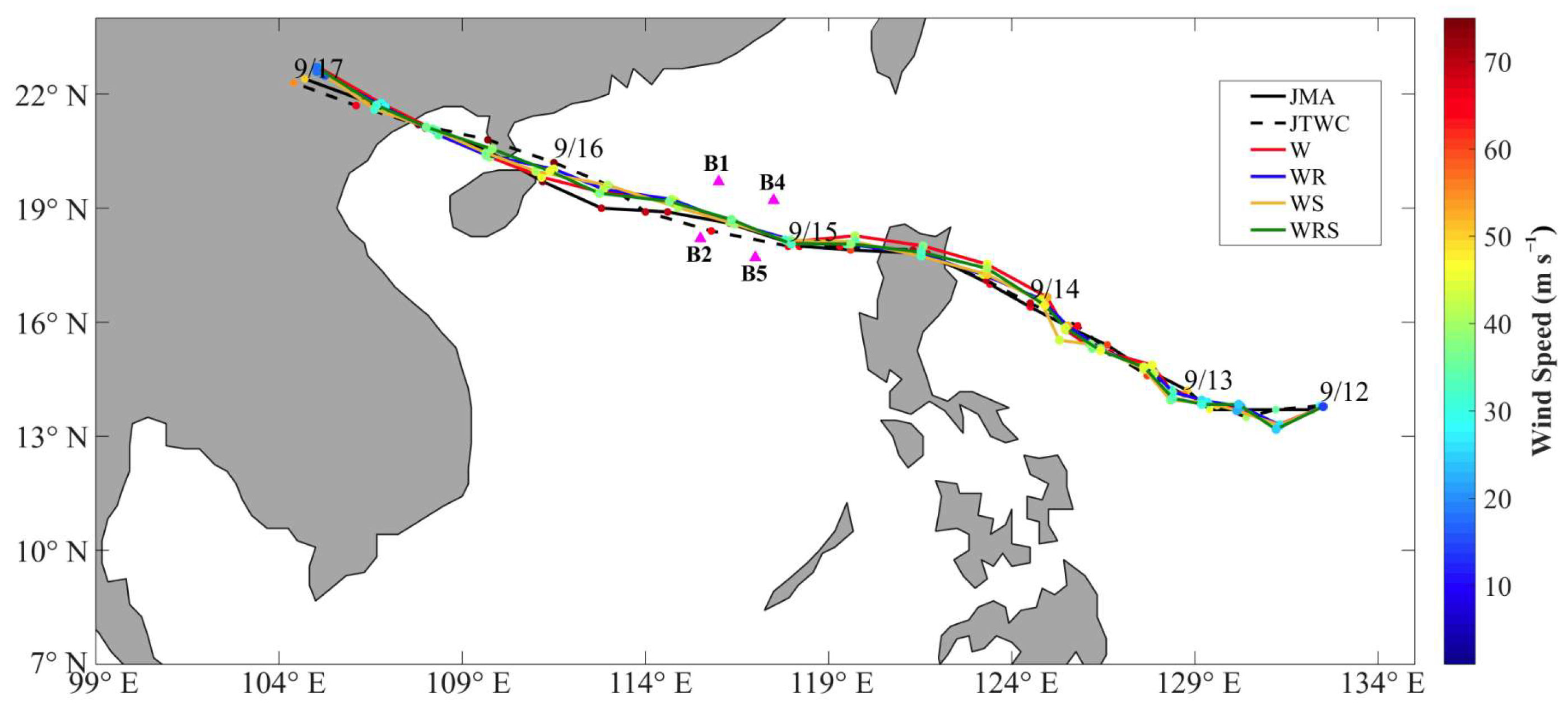
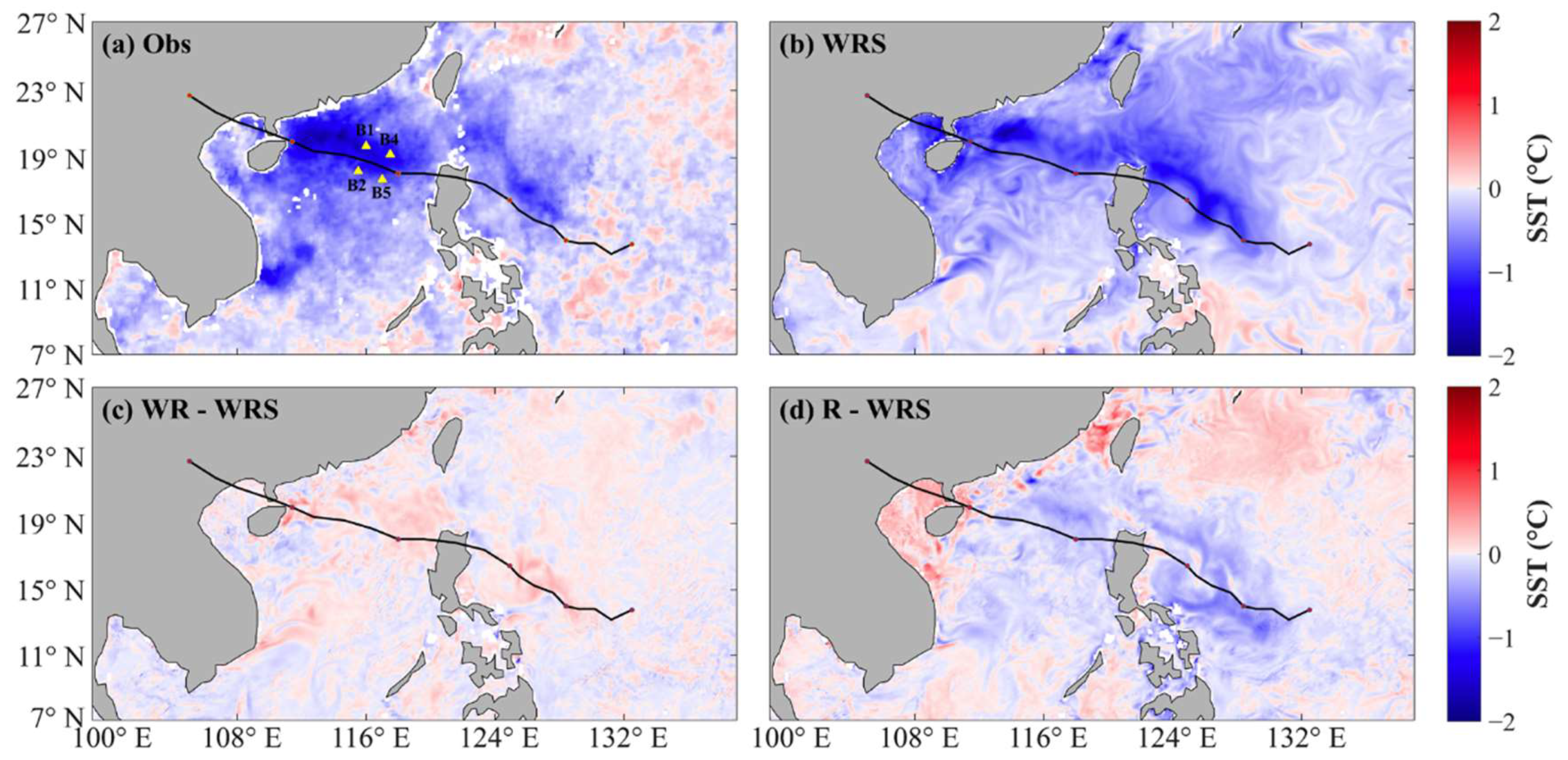
Table 1.
Coordinates and ocean depth at observation points (Buoys 1, 2, 4 and 5) shown as yellow triangles in Figure 1.
Table 1.
Coordinates and ocean depth at observation points (Buoys 1, 2, 4 and 5) shown as yellow triangles in Figure 1.
| Buoy | Longitude (°E) | Latitude (°N) | Water Depth (m) |
|---|---|---|---|
| 1 | 116.0 | 19.7 | 1630 |
| 2 | 115.5 | 18.2 | 3840 |
| 4 | 117.5 | 19.2 | 3690 |
| 5 | 117.0 | 17.7 | 3990 |
Table 2.
List of sensitivity tests. WRF (W), ROMS (R), SWAN (S), WRF-ROMS (WR), WRF-SWAN (WS) and WRF-ROMS-SWAN (WRS).
Table 2.
List of sensitivity tests. WRF (W), ROMS (R), SWAN (S), WRF-ROMS (WR), WRF-SWAN (WS) and WRF-ROMS-SWAN (WRS).
| Experiments | WRF | ROMS | SWAN |
|---|---|---|---|
| W | Yes | No | No |
| R | No | Yes | No |
| S | No | No | Yes |
| WR | Yes | Yes | No |
| WS | Yes | No | Yes |
| * WRS | Yes | Yes | Yes |
* baseline experiment.
Table 3.
Correlation coefficient (R2), root-mean-square difference (RMSD) and skill score (SSc and SSr) for 10-m wind and SLP from the different experiments.
Table 3.
Correlation coefficient (R2), root-mean-square difference (RMSD) and skill score (SSc and SSr) for 10-m wind and SLP from the different experiments.
| Experiments | Wind | SLP | ||||||
|---|---|---|---|---|---|---|---|---|
| R2 | RMSD | SSc | SSr | R2 | RMSD | SSc | SSr | |
| W | 0.9398 | 2.9551 | 0.0011 | −0.0949 | 0.9809 | 1.7682 | −0.0023 | −0.0337 |
| WR | 0.9501 | 2.8357 | 0.0120 | −0.0551 | 0.9813 | 1.7683 | −0.0018 | −0.0338 |
| WS | 0.9209 | 3.0884 | −0.0193 | −0.1211 | 0.9797 | 1.8160 | −0.0034 | −0.0696 |
| WRS | 0.9390 | 2.7859 | 0.0000 | 0.0000 | 0.9831 | 1.7151 | 0.0000 | 0.0000 |
Table 4.
Correlation coefficients (R2), root-mean-square errors (RMSD) and skill scores (SSc and SSr) for SST and ocean surface current from the different experiments.
Table 4.
Correlation coefficients (R2), root-mean-square errors (RMSD) and skill scores (SSc and SSr) for SST and ocean surface current from the different experiments.
| Experiments | SST | Current | ||||||
|---|---|---|---|---|---|---|---|---|
| R2 | RMSD | SSc | SSr | R2 | RMSD | SSc | SSr | |
| R | 0.9736 | 0.2888 | 0.0052 | 0.2923 | 0.8831 | 0.4348 | 0.0099 | −0.1703 |
| WR | 0.9698 | 0.4170 | −0.0012 | −0.0130 | 0.8683 | 0.3524 | −0.0074 | 0.0631 |
| WRS | 0.9687 | 0.4145 | 0.0000 | 0.0000 | 0.8744 | 0.3806 | 0.0000 | 0.0000 |
Table 5.
Correlation coefficients (R2), root-mean-square errors (RMSD) and skill scores (SSc and SSr) for significant wave height from the different experiments.
Table 5.
Correlation coefficients (R2), root-mean-square errors (RMSD) and skill scores (SSc and SSr) for significant wave height from the different experiments.
| Experiments | SWH | |||
|---|---|---|---|---|
| R2 | RMSD | SSc | SSr | |
| S | 0.9489 | 1.0466 | −0.0018 | −0.4104 |
| WS | 0.9488 | 0.8637 | −0.0019 | −0.1621 |
| WRS | 0.9506 | 0.7433 | 0.0000 | 0.0000 |
© 2020 by the authors. Licensee MDPI, Basel, Switzerland. This article is an open access article distributed under the terms and conditions of the Creative Commons Attribution (CC BY) license (http://creativecommons.org/licenses/by/4.0/).
Share and Cite
MDPI and ACS Style
Lim Kam Sian, K.T.C.; Dong, C.; Liu, H.; Wu, R.; Zhang, H. Effects of Model Coupling on Typhoon Kalmaegi (2014) Simulation in the South China Sea. Atmosphere 2020, 11, 432. https://0-doi-org.brum.beds.ac.uk/10.3390/atmos11040432
AMA Style
Lim Kam Sian KTC, Dong C, Liu H, Wu R, Zhang H. Effects of Model Coupling on Typhoon Kalmaegi (2014) Simulation in the South China Sea. Atmosphere. 2020; 11(4):432. https://0-doi-org.brum.beds.ac.uk/10.3390/atmos11040432
Chicago/Turabian StyleLim Kam Sian, Kenny T.C., Changming Dong, Hailong Liu, Renhao Wu, and Han Zhang. 2020. "Effects of Model Coupling on Typhoon Kalmaegi (2014) Simulation in the South China Sea" Atmosphere 11, no. 4: 432. https://0-doi-org.brum.beds.ac.uk/10.3390/atmos11040432
Note that from the first issue of 2016, this journal uses article numbers instead of page numbers. See further details here.