Chemical Composition of PM10 in 16 Urban, Industrial and Background Sites in Italy †


1
Institute of Atmospheric Pollution Research, National Research Council of Italy, Monterotondo st., 00015 Rome, Italy
2
Chemistry Department, Sapienza University of Rome, 00185 Rome, Italy
*
Author to whom correspondence should be addressed.
†
Presented by Cinzia Perrino, Maria Catrambone and Silvia Canepari on behalf of the IIA-SapCD study group.
Atmosphere 2020, 11(5), 479; https://0-doi-org.brum.beds.ac.uk/10.3390/atmos11050479
Submission received: 16 March 2020
/
Revised: 23 April 2020
/
Accepted: 5 May 2020
/
Published: 8 May 2020
(This article belongs to the Special Issue Recent Advances of Air Pollution Studies in Italy)
Abstract
:Italy is characterized by a very variable configuration in terms of altitude, proximity to the sea, latitude and the presence of industrial plants. This paper summarizes the chemical characterization of PM10 obtained from 38 sampling campaigns carried out in 16 sites in Italy during the years 2008–2018. Chemical determinations include all macro-components (six macro-elements, eight ions, elemental carbon and organic carbon). The sum of the individual components agrees well with the PM10 mass. The chemical composition of the atmospheric aerosol clearly reflects the variety in the Italian territory and the pronounced seasonal variations in the meteoclimatic conditions that characterize the country. Macro-sources reconstruction allowed us to identify and evaluate the strength of the main PM10 sources in different areas. On 10 sampling sites, the soluble and insoluble fractions of 23 minor and trace elements were also determined. Principal Component Analysis was applied to these data to highlight the relationship between the elemental composition of PM10 and the characteristics of the sampling sites.

1. Introduction
It is well known that air quality is strongly influenced by atmospheric conditions and that atmospheric conditions partly depend on the geographical location and orography of the site. From this point of view, Italy is a very complex environment, characterized by a wide geographic variability. It extends between 47°04′ and 35°29′ degrees north latitude and includes two great mountain ranges, the Alps, which encompass the northern part of the country, and the Apennine Mountains, which extend for about 1300 km along the peninsular region. It also includes a very wide plain to the north, the Po valley (46,000 km2), and about 7500 km of coastline. This varied landscape reflects in a wide variety of climate systems, which range from the cold, wet winters of the northern mountain areas and the strong winter stability of the Po valley to the mild conditions of the coastal regions, temperated by the breeze, and the long, hot summer in the south of the peninsula.
These different features influence air quality to varying extents. In general, air quality shows a wide variability not only according to the intensity of local emission sources but also as a consequence of the mixing properties of the lower atmosphere, the medium- and long-range transport of the air masses, the frequency and intensity of rainfall. Atmospheric particulate matter (PM), characterized by a very complex chemical composition, size distribution and source variety, is mainly influenced by the various geographical and climatic characteristics of the receptor site. It can thus be intriguing to observe similarities and differences in PM chemical composition among different Italian locations.
In the literature, many papers concern the chemical composition of PM in individual cities or geographic areas of Italy [1,2,3,4,5,6,7,8,9,10,11,12,13,14,15,16]. However, to our knowledge, no studies take into consideration many locations in different areas of the country. Some papers focus on one city only: Milan [2,13], Genoa [3], Venice [8], Bologna [11], Ferrara [9,10], Lecce [16]. Some others compare a small number of sites in the same region (Lazio [4], Apulia [5], Emilia Romagna [14], Veneto [15]) or along the country [1,6]. Some peculiarities of the Italian region are discussed in the paper of Amato et al. [12], where the chemical composition of PM10 and PM2.5 in Milan and Florence is compared with those measured in Barcelona, Athens and Porto. Finally, the paper of Putaud et al. [7], discusses the chemical composition of PM in more than 60 sites across Europe, including four Italian cities, and highlights regional differences in PM characteristics among northwestern, central and southern Europe.
In this paper, we gather an extensive dataset about the mass concentration and chemical composition of PM10 (particulate matter with aerodynamic diameter less than 10 μm) collected during air quality studies carried out in different Italian sites during the period 2008–2018. The sites range from vast urban areas to small mountain villages. We also included some residential sites close to industrial areas, which are not infrequent in Italy.
We obtained the data during sampling campaigns carried out by using identical instrumental equipment and carried out the analyses by following the same analytical procedure. These features make the dataset very homogeneous and allow us to observe the variability of PM10 composition in different geographical and seasonal conditions.
Chemical characterization includes the determination of macro-components (seven macro-elements, eight ionic species, organic carbon, elemental carbon), which allowed us to obtain the mass closure, and 23 micro-elements, able to trace some sources of particular interest. In most cases, we collected the data during two different periods of the year (warm and cold season), for a total of about 1300 samples. To extract more information from the micro-elements dataset, we applied Principal Component Analysis (PCA); in this receptor model, the mathematical functions that best describe the relative distances between the samples are given by the direction with the maximum variance of the data [17].
2. Experiments
2.1. Sampling Sites and Periods
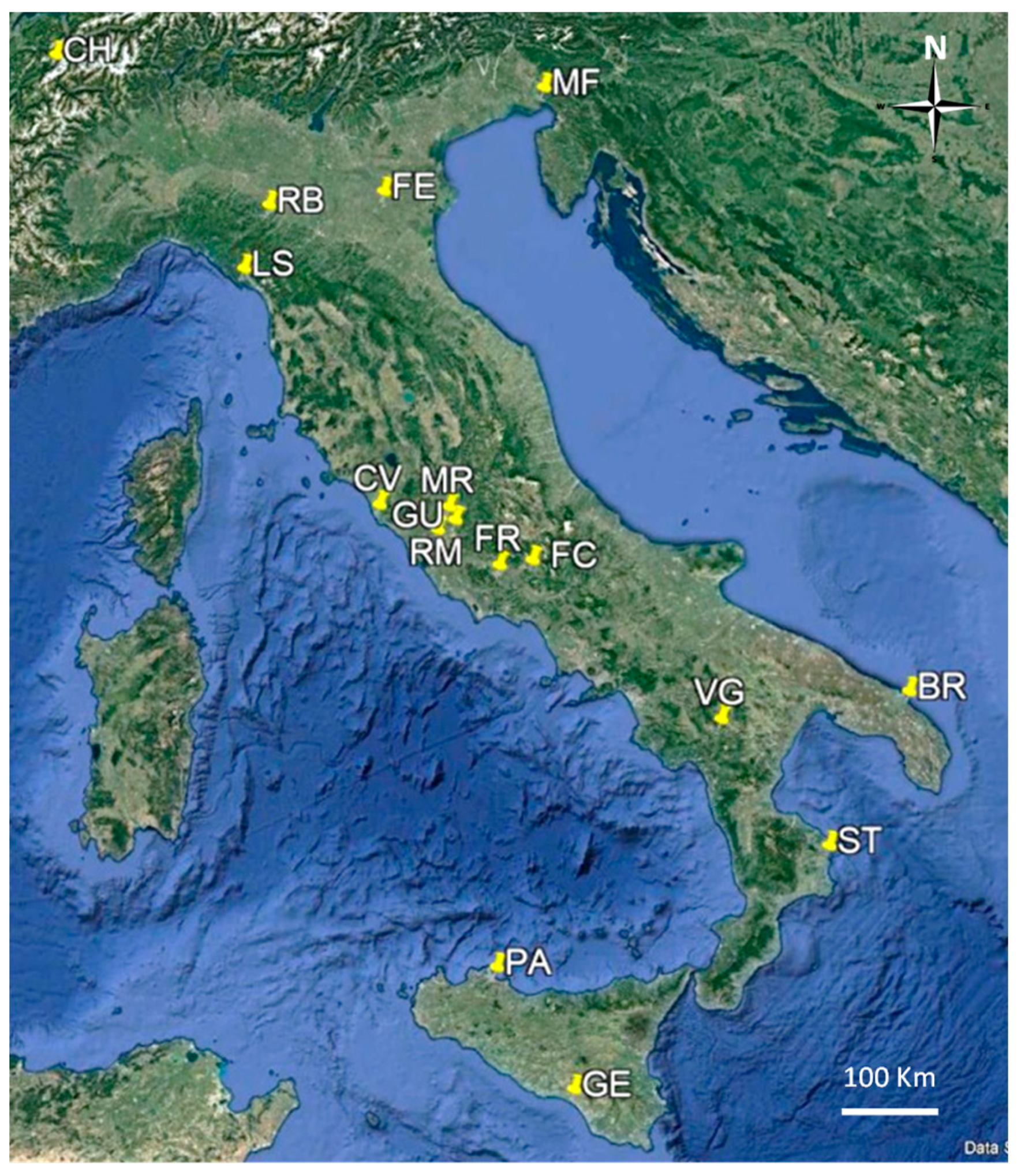
The sixteen sampling sites, shown on the map in Figure 1, are briefly described below, ordered from north to south.
Chamonix (CH) is a mountain village located in a small valley on the Mont Blanc, in a French territory about 8 km from the Italian border. We choose this area as it is representative of the alpine valleys. Monfalcone (MF) is a small industrial city overlooking the northern Adriatic Sea. Its territory includes a coal cogeneration plant, one of the leading shipyards of the Mediterranean and some engineering industries. Ferrara (FE) is a medium-sized town located in the Po valley. We carried out the samplings at about 5 km from Ferrara, in a site close to the industrial area that includes a waste-to-energy plant and a vast petrochemical complex. Rubbiano (RB) is a small village located in a valley surrounded by hills at the southern border of the Po valley. Its industrial area includes food and expanded clay production plants. La Spezia (LS) is one of the most important Italian military and commercial harbours, in the north-western part of the Mediterranean basin. A power plant is located in the area.
Civitavecchia (CV), on the Tyrrhenian Sea, is a major cruise and ferry port; the city is also the seat of two coal-fired thermal power stations. We carried out the samplings on the coastline at about 5 km from the city centre. Monterotondo scalo (MR) is a village located at about 20 Km NE of Rome, in central Italy. Close to the Tiber River, it is surrounded by agricultural areas. We carried out the samples in the Research Area of the National Research Council of Italy, at about 7 km NE from the village. Guidonia (GU) is a medium-sized town at about 20 km for the city of Rome. Its area is characterized by large travertine caves and cement industry. Rome (RM), the most extensive city in the European Union, about 25 km from the Tyrrhenian Sea, is characterized by the absence of heavy industry and by very high vehicular traffic, with about 2,700,000 private cars. The sampling site was inside the Sapienza University, not directly exposed to vehicular traffic. Fontechiari (FC) is a village in central Italy considered by the local Environmental Protection Agency as a regional background. Frosinone (FR) is an industrial and commercial city located on a hill facing the Sacco river valley and surrounded by mountains. Due to its position, the city experiences extreme atmospheric pollution events. We carried out the samplings in the industrial area, close to the river, at about 5 km from the city centre.
Brindisi (BR), on the eastern coast of Italy, is the leader area in electricity production in Italy. Our sampling site was close to a coal cogeneration plant, at about 10 km from the city centre. Viggiano (VG) is a village located in the Val d’Agri valley, a few km from the most extensive oil platform in continental Europe. Strongoli marina (ST) is a sea village in the south of Italy. A biomass power plant is located nearby (2 km). Palermo (PA), in Sicily, is one of the warmest cities in Italy and Europe, experiencing very long, hot and dry summers. It is one of the major passenger traffic harbours in the Mediterranean; it is also characterized by heavy vehicular traffic (about 750,000 private cars). Gela (GE), is located on the southern coast of Sicily. It is surrounded by crops, but it also borders with a large refinery that was still active during the sampling periods. We carried out the samplings at about 3 km from the city centre.
Table 1 reports the main characteristics of the 16 sampling locations, the number of sampling sites in each area, the years when we carried out the samplings and the total duration of the samplings during the warm (W) and the cold (C) periods. Warm and cold periods are defined as 1 April–30 September and 1 October–31 March, respectively.
The Latitude and longitude of the sampling areas and range of the mean daily temperature during the sampling periods considered in this work are reported in the Supplementary Material (Table S1).
2.2. Sampling and Analytical Procedure
PM10 was collected by using a dual-channel automatic monitor (SWAM 5a Dual Channel Monitor, FAI Instruments, Fonte Nuova, Rome, IT) providing the concentration of PM10 by the beta attenuation method. The instrument has been certified as a beta monitor by both the German TÜV (Technischer Überwachungsverein) and the British MCERTS (Environment Agency of England & Wales Monitoring Certification Scheme); it complies with EU equivalence criteria for PM measurements against EN 12341 and EN 14907 reference methods [18]. The two channels were equipped with Teflon membrane filters (TEFLO, 47 mm, 2.0-micron pore size, PALL Life Sciences, New York, NY, USA.) and quartz fibre filters (TISSUQUARTZ 2500QAT, 47 mm, PALL Life Sciences, New York, NY, USA.). Samples were collected daily, from midnight to midnight, at a flow rate of 2.3 m3/h.
After sampling, Teflon filters were analyzed by energy-dispersion X-ray fluorescence (XRF) (X-Lab 2000 and XEPOS, Spectro Analytical Instruments, Kleve, Germany) for Si, Al, Fe, Na, K, Mg, Ca and minor elements. Then, the filters were extracted for 20 min under sonication in 10 mL of deionized water. A total of 1 mL of the solution was analyzed for ions (chloride, nitrate, sulfate, sodium, potassium, ammonium, magnesium, calcium) by ion chromatography (IC) (ICS1000, Dionex Co., CA, USA). The remaining solution was added with 1 mL acetate buffer (CH3COOH/CH3COOK 0.1 M; pH 4.3). The rationale for the use of this extraction solution is widely discussed in Canepari et al. [19]. Briefly, the use of a pH-buffered solution makes the element solubility percentage independent from the concentration of the acidic species in the sample and directly attributable to the chemical form of elements released by each source. The solution was filtered with nitrocellulose filter (0.45 μm pore size) (Merck Millipore Ltd., MA, USA) and analyzed for the extracted fraction of elements (As, Ba, Bi, Cd, Ce, Co, Cs, Cu, Fe, La, Li, Mg, Mn, Mo, Ni, Pb, Rb, Sb, Sn, Ti, Tl, U, V) by inductively coupled plasma mass spectroscopy (ICP-MS) (Bruker 820 MS); the solid residual on both the sampling filter and the filtration filter was subjected to microwave-assisted acid digestion (HNO3:H2O2 2:1), filtered and analyzed by ICP-MS for the same elements (residual fraction). The results obtained for the two chemical fractions were added to get the total elemental concentration. A full description of the analytical procedure is reported in Canepari et al. [19,20].
Quartz filters were devoted to the analysis of elemental and organic carbon by thermo-optical analysis (OCEC Carbon Aerosol Analyser, Sunset Laboratory, OR, USA), applying the NIOSH–QUARTZ temperature protocol. In the case of site CH, a 1.5 cm2 punch of the filter was extracted in de-ionized water and analyzed for levoglucosan by High-Performance Anion-Exchange Chromatography with Pulsed Amperometric Detection (HPAEC-PAD) [21].
The analytical performances of the overall method were widely checked in its development stage and are reported in previous papers [22,23]. In the case of Mg and Fe, the measurements were carried out by both XRF and ICP. The results of the comparison between the two datasets considered in this work show good correlation for both elements and agree with those previously reported in Canepari et al. [23]: Mg:R2 = 0.93, slope = 1.18; Fe:R2 = 0.82, slope = 0.90.
We carried out explorative PCA using the statistical software CAT (Chemometric Agile Tool [24]) based on the R-project for statistical computing, Ver. 3.0, 32-bit. The data matrix was transformed by performing row and column autoscaling to correct for variations in the different scaling of the examined variables.
3. Results and Discussion
3.1. Macro-Components
For each PM10 sample, we checked the mass closure, that is the correspondence between the concentration of PM10 measured by beta attenuation and the concentration reconstructed by adding the main PM components. To account for non-measured elements (typically H, O), in this calculation, we applied some conversion factors. The rationale for the choice of the conversion factors is widely discussed in the review of Chow et al. [25] and is reported in the Supplementary Material (SM1). Briefly, we considered elements as oxides [26,27]), calculated carbonate as the sum of calcium ion multiplied by 1.5 and magnesium ion multiplied by 2.5, and multiplied organic carbon (OC) by a conversion factor to take into account non-C atoms in organic molecules and obtain organic matter (OM). The conversion factor of OC to OM was set as 2.1 for the agricultural background site FC, 1.6 for urban sites (LS, GU, PA) and 1.8 for all the other sites (residential and peri-urban) [28,29]. In the case of Rome, we applied factor 1.8 because the sampling sites were inside the university area, not directly exposed to traffic emission.
The comparison between the concentrations measured by beta attenuation and reconstructed from the chemical analysis is reported in the Appendix A (Figure A1). The agreement between the two data series is very satisfactory (slope: 0.95; intercept: 0.09; R2 = 0.96; N= 1293) and this ensures that the analytical results were of good quality and all the macro-components were included and confirms that the conversion coefficients for elements and organic carbon were appropriate.
The mean, median, 10th and 90th percentile of the analytical values are reported for all sites in Appendix B, Table A1, for the cold period of the year and Table A2 for the warm period. The data show that, in most cases, the variability of the concentrations, estimated as the ratio between 90th and 10th percentile, is in the range 2–5. Moreover, the difference between the mean and the median value is small and almost centred between the two percentiles, indicating that the concentration distribution is nearly symmetrical. As expected, the concentration variability is higher in the case of natural PM components, such as Al, Si, Na+, Cl−. This variability is the consequence of the desert dust and sea-spray transport events that often occur in central-south areas and coastal areas of the country, respectively [5,16].
Considerable variability is also observed for nitrate and ammonium concentration at site MF during the cold season. This difference, which is also reflected in PM10 mass, is due to very different meteorological conditions occurring at this site during the two winter sampling periods. During the first one (12–25 February 2015), meteorological conditions in the area were characterized by moderate air mixing during both daytime and nighttime hours (mean wind velocity during the period: 1.0 m s−1; range of the daily mean: 0.1–2.8 m s−1). During the second one (22 January–4 February 2016), instead, conditions of windless calm and extreme atmospheric stability occurred during the whole period (mean wind velocity during the period: 0.25 m s−1; range of the daily mean; <0.1–1.1 m s−1), being responsible for the build-up of all atmospheric pollutants and favouring the formation and accumulation of secondary PM components. For this reason, in the following discussion, the two sampling periods at MF are considered separately.
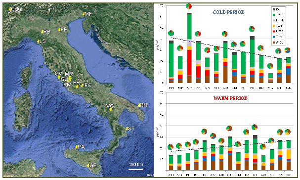
For a more straightforward discussion and interpretation of the data, in Figure 2, we report the mean concentration recorded at the 16 sites during the cold period (Figure 2a) and the warm period (Figure 2b), ordered from north to south. For interpreting macro-components’ concentration, we decided to combine components in the case of natural sources (soil and sea) and to keep the rest of the parameters as individual components. Soil contribution was calculated by summing the concentration of elements (as metal oxides) that are generally associated with mineral dust: Al, Si, Fe plus the insoluble fractions of K, Mg and Ca (calculated as the difference between the XRF and the IC determinations), plus calcium and magnesium carbonate. Sea-salt contribution was calculated from the concentration of soluble sodium and chloride, determined by IC, multiplied by 1.176 to take into account minor seawater components (sulphate, magnesium, calcium, potassium) [28,29,30]. It is conceivable that this procedure neglects some minor sources (e.g., brake dust in the case of Fe), but it is suitable to get a comprehensive estimation of the relative weight of the main, ubiquitary PM sources. In the case of organic species, we report OM concentration, obtained by applying the same multiplication coefficients used for getting the reconstructed mass.
Although some variability in the results is certainly due to the different atmospheric conditions during the various sampling periods, which are not simultaneous, the data allow for the evaluation of some general trends. During the cold period, the data show a wide concentration variability among sites (up to 7–8 fold). This depends on the wide variability of meteorological conditions during the cold seasons, which span from windy and rainy days, which cause pollution reduction, to atmospheric stability periods, when the concentration of PM components, mainly secondary species, quickly increases [2,14,31]. This second condition is typical of plains surrounded by hills/mountains that limit air circulation. From a general point of view, the data show a concentration decrease with increasing latitude. Different to the northern areas, the higher temperatures and the milder conditions that occur in the south, due to the proximity to the sea, promote atmospheric mixing and impair the occurrence of long periods of atmospheric stability.
The individual differences in the composition of PM10 among areas depend on the peculiar geographical position of the sampling site and the local sources. Concerning soil, the concentration is particularly high at GU, due to the presence of travertine caves. When moving from north to south, the percent contribution of soil components tends to increase as a result of increasing soil dryness. In the urban area of Rome (RM), instead, the relevance of soil components (about one-quarter of the total PM10 concentration) is the result of traffic-induced soil re-suspension.
The per cent contribution of sea-salt ranges from a few percentage points in areas far from the sea, to about 25% in Sicily (GE). However, the contribution of this source is strongly dependent on the occurrence of transport events during the sampling campaign, and it is thus very variable as a function of the observation period [14].
Concerning inorganic secondary components, the widest variation is observed for nitrate, whose mean concentration ranges from below 1 μg/m3 at VG to more than 20 μg/m3 at MF during the second sampling period. The highest values are recorded in the Po valley and surrounding areas (MF, FE, RB), where a high concentration of precursors (NH3 and NOx) adds to high atmospheric stability and humid climate in favouring the production of ammonium nitrate [14,32]. The contribution of sulphate (in the form of ammonium salts) is generally low due to the low sulphur content of fossil fuels used in the country. Sulphate contribution above 10% are recorded at MF (second period), BR and VG. Here, the role of the industrial plants, whose SO2 emissions can be quickly transformed into sulphate, is probably not negligible (coal cogeneration plants at MF and BR and oil platform at VG). In Sicily, SO2 emission from the Etna volcano and from ships may also give a contribution.
The concentration of organic components shows wide variability, but their contribution to PM10 is high everywhere (on average, about 50%). One of the main winter sources of organics can be identified in biomass burning [12,33,34,35,36]. The highest values (30.2 μg/m3) and highest per cent OM contributions (78%) were recorded at CH, an Alpine village made of small houses heated by fireplaces and stoves. During this campaign, we also determined levoglucosan, a reliable tracer of biomass burning, and found an average concentration as high as 2 μg/m3, (range 0.75–3.2 μg/m3), indicating that this source was responsible, on average, for more than 50% of the organic mass. We recorded very high OM contributions also at FC (70%) and FR (58%), both located in areas where biomass burning is frequently used for domestic heating.
EC concentration and percent contribution are high at RM (9%) and FR (8%), where traffic emission is particularly intense, but also at CH (7%), as a consequence of both the proximity to the Mont Blanc Tunnel and the very high contribution of biomass burning.
During the warm period (Figure 2b), the concentrations in northern Italy are much lower than during the cold season, while they are only slightly lower in the south. Differently from the cold period, during the warm season, a general increase in concentration is observed when moving from north to south. This behaviour is mainly due to the higher temperature and solar radiation occurring at the lower latitudes, which result in the soil being dryer and more intense photochemical activity. During the cold season, besides, atmospheric stability periods generally occurring in northern regions are much less frequent and severe.
In comparison with the cold season, increased soil contribution to PM10 is observed all over the country, with an average value of about one third. In this case, as well, the highest concentration and contribution are recorded at GU. The contribution of sea-salts is very variable, as discussed for the cold period, but it is generally higher at the three harbours (LS, CV, PA). Nitrate is the component that experiences the widest concentration reduction from the cold to the warm semester, as the equilibrium between particulate ammonium nitrate and ammonia and nitric acid in the gaseous phase is sensitive to the temperature. Moreover, the reduction in NOx emissions from traffic and domestic heating may play a role [16]. Conversely, ammonium sulphate concentration increases during the warm period, due to photochemical conversion of SO2, particularly in areas (LS, PA, GE) where SO2 concentration is influenced by local emission sources (fossil fuel combustion from ship and power plants and, in Sicily, the Etna volcano) [5,16,37]. Organic matter also shows a significant concentration decrease during the warm period, despite the increase in photochemical bioVOCs oxidation. This confirms, once again, the relevance of the contribution of biomass burning for domestic heating, which switches off during the warm months. The decrease in nitrate and OM concentration is the main factor responsible for the general reduction in PM10 concentration during the warm period. EC concentration values are very similar to those recorded during the cold period, and percent contribution is slightly higher due to the reduction in the concentration of the other components.
Our findings are in good agreement with those of the AIRUSE project [12]: the average composition in Milan (OM 38%, EC 5%, sulphate 7%, nitrate 14%, ammonium 8%, sea-salt 2%, soil dust 9%) are in the range of our results for northern Italy. In the same paper, the chemical composition in Milan (in the Po valley) and in Florence (located in a closed basin in Central Italy) showed higher PM10 levels (by a factor of more than 2) in autumn and winter with respect to the warm season and the cities of Athens, Barcelona and Porto. These high levels were attributed to the stagnant meteorological conditions that prevail in Milan and Florence during the cold period. Very high PM10 values in comparison with the 60 European examined locations were also recorded in the Po valley (Bologna) by Putaud et al. [7].
3.2. Micro- and Trace- Elements
The analysis of micro- and trace- elements was carried out on a subset of sites: MF, FE, RB, RM, BR, VG, ST, GE (cold period) MF, FE, RB, LS, CV, RM, GE (warm period). The mean, median, 10th percentile and 90th percentile of the concentrations are reported, for all sites, in Appendix C, Table A3, for the cold period of the year and Table A4 for the warm period.
Also in this dataset, the mean and median concentration values are generally very close to each other and in the middle range to the 10th and 90th percentiles, suggesting a symmetrical distribution of the data. As observed for the macro-components, the two winter periods at MF show very different results, with elemental concentration 2–4 times higher during the second campaign. In general, a higher variability range of the elemental concentrations is observed with respect to macro-components (ratio between 90th and 10th percentile up to about 10). This variability is probably due to the higher sensitivity of micro-components to local or discontinuous minor PM sources, which may show a wide strength variability in time (sources that have a small impact on PM mass concentration but may significantly affect the concentration of micro-tracers).
In the case of sites MF, FE, RB, RM and GE, it is possible to discuss the seasonal variations. In agreement with the behaviour observed for macro-components, the data show that the occurrence of atmospheric stability conditions has a definite effect on the measured concentration, mainly in sites that experience severe episodes (Po valley: MF and FE). The ratios between the cold and the warm periods widely exceed unity at MF (second campaign), FE and RM, mainly for elements related to industrial activities (As, Bi, Cd, Ni, Pb, Sn), traffic emission (Ba, Cu, Fe, Mo, Sb) and biomass burning (Cs, Rb, Tl) [10,36,38,39]. The difference along the year is instead negligible in the other sites (RB and GE).
For a more straightforward interpretation of the results, we run the PCA on the elemental concentration obtained by ICP-MS; in this case, we considered the two MF winter sampling periods separately. In this analysis, we chose not to perform PCA on individual campaigns but to include all the available data. This choice does not allow a reliable source apportionment in individual sites because each studied area is characterized by different, peculiar sources. However, it permits the easy, visual identification of differences and similarities in the elemental composition of PM among the considered sites.
PCA analysis extracted six components, able to explain 81.1% of the total variance; the loadings are reported as Supplementary Material (Table S2).
The first component, which explains 44.5% of the variance, mainly reflects the overall variation in PM concentration; the score and loading plot of Components 1 and 2 are reported in the Supplementary Material (Figure S1).
Figure 3 shows the score plot (a) and loading plot (b) of Components 2 and 3, which explain 15.8% and 8.1% of the variance, respectively. The elemental composition clearly differentiates the sites: the samples taken at each site group in a different area of the score plot, independently from the period of the year when they were collected. In particular, the samples collected at MF, FE, CV and RM are well separated from each other. MF data are found in the upper-right quarter of the score plot; in the loading plot, this area corresponds to elements of industrial origin (Bi, As, Mo, Cd, Sn, Pb). The same elements, probably with different relative weight, also characterize FE results (upper side of the score plot). The RM samples (upper-left side of the score plot) correspond, as expected, to the area of the loading plot where traffic elements group (Cu, Sb). In the literature, Cu/Sb is widely considered as a diagnostic ratio of traffic sources, with values around 4–5 [40]. Our data show that, in sites with a high traffic intensity (LS, RM, but also MF and FE), this ratio is much higher than 4 (range 7–12). These higher Cu/Sb values are probably due to the phasing-out of Sb from brake pads, due to the growing concern about Sb adverse effects on health [41]. Finally, CV samples spread over the left side of the score plot and are characterized by high concentrations of La, Ce, Ba, U, Mg and V.
Many literature studies have shown that the chemical fractionation of elements is a robust tool to increase their performance as source tracers [10,42]. In particular, combustion/industrial sources were found to release elements as chemical species that are generally more soluble than those released by abrasive processes, such as non-exhaust traffic emission [11,42,43,44,45,46]. The descriptive statistics of the concentration of the elemental soluble fraction during the two seasonal periods is reported as Supplementary Material (Tables S3 and S4). In Figure 4, we report the results of the PCA, run on the soluble fraction of elements, considering all sites and periods. Considering that this fraction is mainly associated with combustion/industrial sources, it is reasonable to think that that it is more effective in separating these contributions.
In this case, as well, we considered six components, explaining 73.1% of the total variance; the loadings are reported as Supplementary Material (Table S5). Again, the first component, which explains 36.0% of the variance, reflects only the variation in element concentration; the score and loading plot of Components 1 and 2 are reported in Supplementary Material (Figure S2). Figure 4 shows that MF results group in the upper-left part of the score plot and are well separated from FE data. In the loading plot, they correspond to Sn, Fe, Bi and Li, elements that typically are of industrial origin. It is worth noting that, despite the very different concentration levels recorded at MF during the two winter sampling periods, all the MF data align on the same trajectory. This finding further confirms that the stability of the atmosphere can increase/decrease pollutants’ concentration, but, in the case of primary pollutants, it does not alter the elemental profile. FE samples, instead, are grouped in the upper-right quarter of the score plot and correspond, in the loading plot, to a different group of industrial elements: Cd, As and Pb. These elements are recognised as reliable tracers of waste-to-energy plants [47]. It is interesting to note, however, that in a previous paper we showed that in the area of FE the concentration of these elements does not seem to be directly related to local sources but is homogeneous over a vast territory [10].
On the lower side of the score plot, we find LS, CV, GE, all sited on the coastline and close to a coal power plant or an oil refinery. In the loading plot, this area corresponds to Ni and V, related to heavy oil combustion [48,49]. Our data (Appendix C) show that, in agreement with the literature, the Ni/V ratio is lower in coastal sites. At LS, CV, BR, GE, the value of Ni/V it is well below one, while, in all the other cases, it is higher than one and increases during the cold period. It has been suggested that this increase may be influenced by biomass burning [50,51].
Further information about the variability of the source strength can be obtained by considering the solubility percentage of the elements. As reported in previous papers [10,42], the solubility percentage of each element is strictly dependent on its chemical form, which, on its turn, is typical of the source that has emitted the aerosol in the atmosphere. Variation in the solubility of elements therefore indicates variation in the relative strength of the aerosol sources. The descriptive statistics of the percent solubility of each element during the two seasonal periods are reported in the Supplementary Material, Tables S6 and S7. The data show that the solubility percentage is largely associated with the considered element. The soluble fraction typically constitutes more than 75% in the case of Cd and Tl and less than 25% for Bi, Ce, Fe, La, Sn, Ti, U, while the remaining elements are more distributed between the two fractions. However, we observe a certain variability in the solubility that is due to the different strength of individual sources in the various sites and periods. To evaluate these issues in our dataset, we run the PCA on the solubility percentage (six components, explaining 74.9% of the total variance; loadings in Supplementary Material, Table S8).
Our results confirm that the chemical fractionation increases the ability of elements to trace PM sources, as the PCA run on the solubility percentage provides better separation among sites than the PCA run on concentrations. As an example, we report, in Appendix D (Figure A2), the 3D score plot of Components 3, 4 and 5, where all the sites appear well separated from each other.
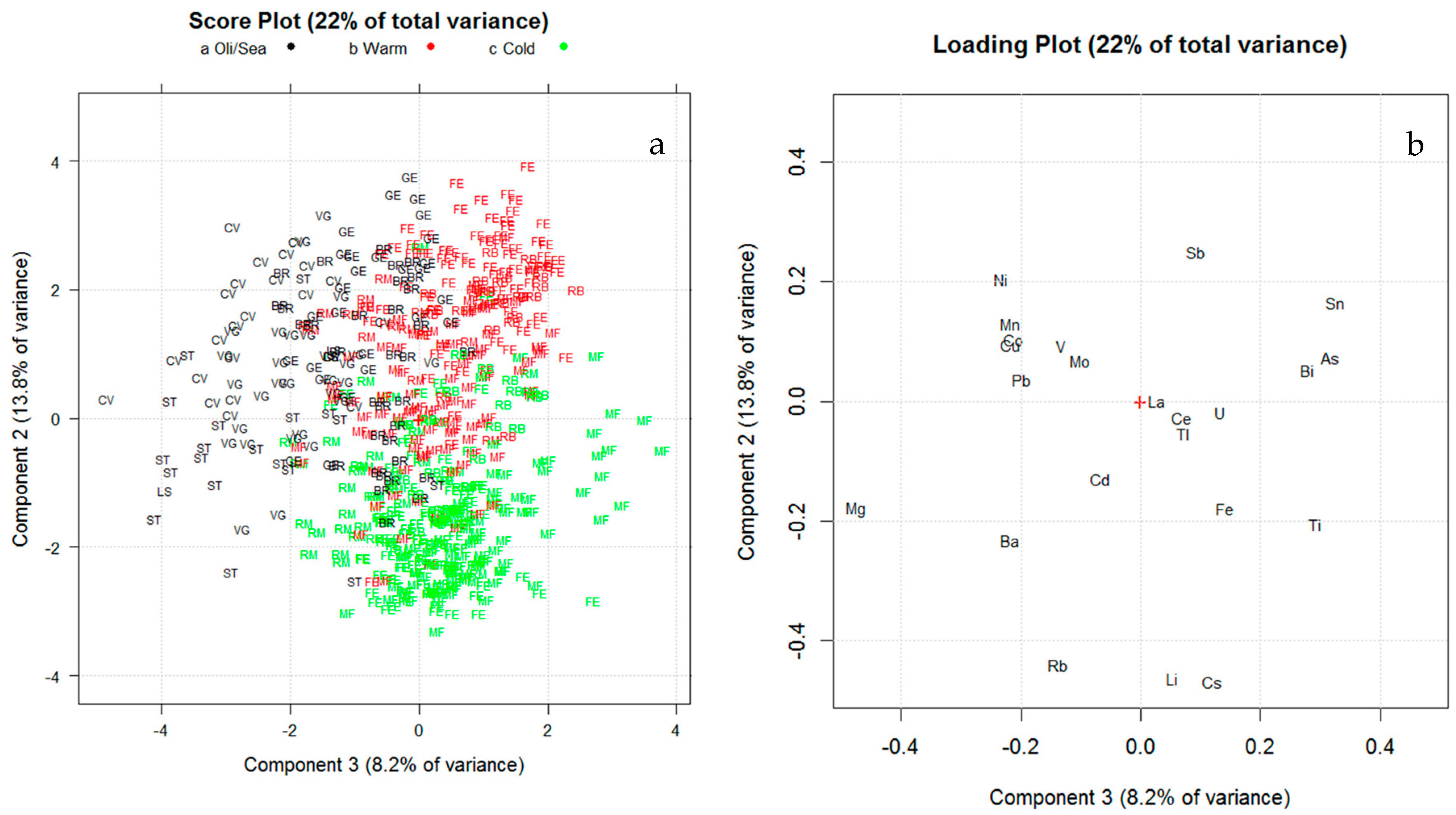
Figure 5 shows the score plot and loading plot f the solubility percentage for Components 2 and 3 (13.8% and 8.1%, respectively, of the total variance). The score and loading plot of Components 1 and 2 are reported in the Supplementary Material (Figure S3).
For sites MF, FE, RB, RM (inland), the cold period is drawn in green and the warm period in red. For sites LS, CV, VG, ST, GE, (coastal/petrochemical), instead, the data are drawn in black, independently of the season. The three groups take up different areas of the graph. Samples collected during the cold semester in inland areas are grouped in the lower-right quarter of the plot and correspond, in the loading plot, to high values of the soluble fraction of Rb, Cs and Li, which is a robust tracer of biomass burning [36,39]. Samples collected during the warm semester in inland sites (upper-right quarter) correspond to a high solubility of As, Sn, Sb e Bi. As discussed above, the soluble fraction of these elements traces industrial sources. Coastal/petrochemical sites, instead, do not show any significant seasonal difference in solubility percentage, as they are mostly influenced by the solubility of elements released by sea-spray (Mg) or by vessel traffic (Ni and V). In facts, Mg in sea-spray is in the form of the soluble MgCl2, and Ni and V in particles emitted by heavy oil-fuelled sources are generally more soluble than elements released by other sources.
4. Conclusions
We investigated the variability of PM10 composition in 16 sampling areas in Italy using both mass closure and a PCA receptor model. Variability between cold and warm periods and among sites was observed, reflecting the geographical position of the site and the influence of the local sources.
A yearly PM10 concentration gradient is recorded all over the country, with a decreasing concentration from north to south during the cold season and an increasing concentration during the warm season. Soil components increase in the same direction. They also increase during the warm semester, as a consequence of soil dryness. Very high ammonium nitrate concentrations are recorded in the Po valley during the cold period, while ammonium sulphate increases during the warm period, mainly in southern and coastal sites. Traffic contribution is more evident in urban areas, particularly in Rome, in the form of both direct exhaust emission and re-suspension. The contribution of organics is very high everywhere, but a significant concentration decrease is observed during the warm season, indicating a relevant contribution of biomass burning during the winter.
As expected, the concentration of micro- and trace elements is mainly driven by the strength of local sources. The elemental profiles are enriched in elements of industrial origin (Bi, As, Mo, Cd, Sn, Pb) at MF (power plant, shipyards, engineering industries) and FE (waste-to-energy plant, petrochemical complex), in elements from traffic exhausts and re-suspension (Ba, Cu, Fe, Mo, Sb) at the urban sites (LS, RM), in Ni, V and Mg at the coastal sites (LS, CV, BR, GE). The study of the soluble fraction of elements, which trace combustion sources more efficiently, allowed for better differentiation between industrial sites (MF and FE). Solubility percentage has been shown to be a robust tool for the identification of PM sources by elemental analysis. We observed a significant increase in the elemental solubility of some tracers of biomass burning (Rb, Li, Cs) during the cold season, as the switch-on of this seasonal PM source causes a substantial increase in their solubility.
Supplementary Materials
The following are available online at https://0-www-mdpi-com.brum.beds.ac.uk/2073-4433/11/5/479/s1, SM1: Rationale for the choice of conversion factors; Figure S1: PCA of elemental concentration (all data): score plot (left panel) and loading plot (right panel) of components 1 and 2. _C and _W after the site code indicate the cold and warm periods, respectively. In the case of MF, the two winter periods are reported as _C1 and _C2; Figure S2: PCA of the soluble fraction of elements (all data): score plot (left panel) and loading plot (right panel) of Components 1 and 2; Figure S3: PCA of the solubility percentage of elements (all data): the score plot (left panel).and loading plot (right panel) of Components 1 and 2; Table S1: Latitude, longitude of the sampling sites and mean temperature during the sampling periods; Table S2: Loadings of PCA run on the total elemental concentrations; Table S3: Concentration of the micro- and trace elements (ng/m3) in the soluble fraction during the cold period; Table S4: Concentration of the micro- and trace elements (ng/m3) in the soluble fraction during the warm period; Table S5: Loadings of PCA run on the soluble fraction of elements, Table S6: Percent solubility of micro- and trace elements during the cold period; Table S6: Percent solubility of micro- and trace elements during the cold period; Table S7: Percent solubility of micro- and trace elements during the warm period; Table S8: Loadings of PCA run on the solubility percentage of elements; Figure S3: PCA of the soluble fraction of elements (all data): score plot (left panel) and loading plot (right panel) of components 1 and 2.
Author Contributions
Project supervision, C.P.; conceptualizzation, C.P. and S.C.; writing, C.P. and S.C.; supervision (IIA study group), C.P.; supervision (SapCD study group), S.C.; sampling campaigns supervision, M.C.; analytical supervision, M.C.; sampling activity, IIA study group; analytical activity and data elaboration, IIA-SapCD study group. All authors have read and agreed to the published version of the manuscript.
Funding
This research received no external funding.
Acknowledgments
The Authors are indebted to T. Davanzo, M. Palozzo and E, Zappaterreno for their administrative support. IIA-SapCD study group: S. Dalla Torre, M. Giusto, F. Marcovecchio, S. Pareti, E. Rantica, T. Sargolini, L. Tofful (IIA); M.L. Astolfi, D. Frasca, M.A. Frezzini, M. Marcoccia, L. Massimi, G. Simonetti (SapCD).
Conflicts of Interest
The authors declare no conflict of interest.
Appendix A
Figure A1.
Scatter plot of PM10 concentration as measured by β attenuation and as reconstructed by the sum of the chemical analyses.
Figure A1.
Scatter plot of PM10 concentration as measured by β attenuation and as reconstructed by the sum of the chemical analyses.

Appendix B

Table A1.
Concentration (mean, median, 10th and 90th percentile) of the main PM10 components, in μg/m3, during the cold period.
Table A1.
Concentration (mean, median, 10th and 90th percentile) of the main PM10 components, in μg/m3, during the cold period.
| Site Samples | Statistics | Al | Si | Fe | K | Mg | Ca | Cl− | NO3− | SO42− | Na+ | NH4+ | K+ | Mg2+ | Ca2+ | OC | EC |
|---|---|---|---|---|---|---|---|---|---|---|---|---|---|---|---|---|---|
| CH N = 14 | MEAN | 0.05 | 0.27 | 0.34 | 0.27 | < 0.02 | 0.35 | 0.48 | 1.3 | 0.94 | 0.31 | 0.45 | 0.24 | 0.014 | 0.25 | 16.8 | 2.8 |
| MEDIAN | 0.04 | 0.18 | 0.32 | 0.27 | < 0.02 | 0.33 | 0.33 | 1.3 | 0.91 | 0.21 | 0.44 | 0.26 | 0.014 | 0.26 | 15.6 | 2.8 | |
| 10th | 0.02 | 0.05 | 0.06 | 0.13 | < 0.02 | 0.10 | 0.21 | 0.72 | 0.67 | 0.13 | 0.25 | 0.11 | 0.004 | 0.070 | 9.6 | 1.8 | |
| 90th | 0.12 | 0.65 | 0.58 | 0.41 | < 0.02 | 0.75 | 1.1 | 1.8 | 1.2 | 0.68 | 0.62 | 0.36 | 0.026 | 0.51 | 25.0 | 3.9 | |
| MF N = 107 | MEAN | 0.12 | 0.38 | 0.39 | 0.61 | 0.08 | 0.95 | 0.22 | 13 | 3.4 | 0.24 | 4.1 | 0.49 | 0.060 | 0.85 | 9.4 | 0.96 |
| MEDIAN | 0.12 | 0.34 | 0.26 | 0.48 | 0.07 | 0.67 | 0.13 | 4.0 | 3.4 | 0.23 | 1.9 | 0.38 | 0.050 | 0.64 | 7.6 | 0.90 | |
| 10th | 0.07 | 0.18 | 0.09 | 0.24 | 0.04 | 0.23 | 0.032 | 0.48 | 0.93 | 0.086 | 0.36 | 0.19 | 0.019 | 0.28 | 3.6 | 0.31 | |
| 90th | 0.18 | 0.63 | 0.94 | 1.17 | 0.14 | 1.88 | 0.51 | 37 | 6.6 | 0.42 | 11.1 | 0.99 | 0.11 | 1.7 | 16.9 | 1.6 | |
| FE N = 82 | MEAN | 0.14 | 0.47 | 0.25 | 0.60 | 0.12 | 0.75 | 0.45 | 11 | 2.3 | 0.28 | 2.9 | 0.24 | 0.056 | 0.66 | 9.2 | 1.0 |
| MEDIAN | 0.13 | 0.39 | 0.20 | 0.53 | 0.10 | 0.56 | 0.33 | 8.4 | 2.1 | 0.23 | 2.5 | 0.26 | 0.053 | 0.53 | 8.4 | 0.91 | |
| 10th | 0.07 | 0.20 | 0.08 | 0.32 | 0.05 | 0.22 | 0.069 | 2.3 | 0.83 | 0.093 | 0.72 | 0.020 | 0.013 | 0.20 | 4.7 | 0.61 | |
| 90th | 0.21 | 0.83 | 0.49 | 1.04 | 0.22 | 1.40 | 0.85 | 23 | 4.0 | 0.52 | 5.9 | 0.53 | 0.11 | 1.4 | 15.6 | 1.7 | |
| RB N = 21 | MEAN | 0.32 | 1.30 | 0.43 | 0.38 | 0.23 | 0.87 | 0.30 | 5.0 | 0.99 | 0.30 | 1.4 | 0.31 | 0.047 | 0.33 | 4.5 | 0.58 |
| MEDIAN | 0.19 | 0.80 | 0.30 | 0.34 | 0.16 | 0.77 | 0.23 | 4.4 | 0.80 | 0.26 | 0.90 | 0.27 | 0.039 | 0.28 | 4.1 | 0.60 | |
| 10th | 0.10 | 0.30 | 0.09 | 0.18 | 0.07 | 0.29 | 0.063 | 0.62 | 0.27 | 0.090 | 0.18 | 0.15 | 0.015 | 0.17 | 2.5 | 0.33 | |
| 90th | 0.63 | 2.63 | 0.88 | 0.59 | 0.41 | 1.55 | 0.72 | 11 | 2.2 | 0.64 | 3.1 | 0.47 | 0.090 | 0.56 | 7.5 | 0.73 | |
| MR N = 55 | MEAN | 0.16 | 0.53 | 0.26 | 1.13 | 0.16 | 0.83 | 0.52 | 2.9 | 1.8 | 0.60 | 0.46 | 0.87 | 0.086 | 0.57 | 8.4 | 0.77 |
| MEDIAN | 0.10 | 0.33 | 0.23 | 1.00 | 0.11 | 0.70 | 0.19 | 2.9 | 1.6 | 0.42 | 0.35 | 0.83 | 0.064 | 0.49 | 8.4 | 0.81 | |
| 10th | 0.06 | 0.15 | 0.14 | 0.31 | 0.04 | 0.17 | 0.056 | 0.83 | 0.97 | 0.093 | 0.13 | 0.15 | 0.018 | 0.18 | 3.1 | 0.22 | |
| 90th | 0.24 | 0.86 | 0.37 | 1.97 | 0.31 | 1.46 | 1.3 | 4.6 | 2.7 | 1.3 | 0.86 | 1.6 | 0.20 | 0.89 | 15.1 | 1.2 | |
| GU N = 28 | MEAN | 0.25 | 1.03 | 0.56 | 0.58 | 0.13 | 4.44 | 0.56 | 3.5 | 3.0 | 0.66 | 0.32 | 0.52 | 0.11 | 3.4 | 8.6 | 1.7 |
| MEDIAN | 0.23 | 1.02 | 0.58 | 0.57 | 0.13 | 4.13 | 0.12 | 3.3 | 2.2 | 0.38 | 0.30 | 0.46 | 0.089 | 2.9 | 7.2 | 1.5 | |
| 10th | 0.09 | 0.38 | 0.15 | 0.24 | 0.06 | 1.51 | 0.073 | 1.4 | 1.0 | 0.17 | 0.13 | 0.21 | 0.041 | 1.1 | 3.3 | 0.53 | |
| 90th | 0.43 | 1.80 | 1.03 | 0.99 | 0.20 | 7.50 | 1.4 | 5.8 | 6.5 | 1.3 | 0.51 | 0.93 | 0.18 | 6.7 | 16.3 | 2.6 | |
| RM N = 42 | MEAN | 0.15 | 0.58 | 0.58 | 0.46 | 0.18 | 1.14 | 1.0 | 1.9 | 1.2 | 0.82 | 0.38 | 0.27 | 0.12 | 0.59 | 6.9 | 2.6 |
| MEDIAN | 0.11 | 0.43 | 0.51 | 0.39 | 0.12 | 0.91 | 0.23 | 1.5 | 1.0 | 0.39 | 0.25 | 0.23 | 0.052 | 0.45 | 6.7 | 1.9 | |
| 10th | 0.07 | 0.23 | 0.14 | 0.21 | 0.06 | 0.45 | 0.043 | 0.58 | 0.33 | 0.091 | 0.092 | 0.078 | 0.020 | 0.23 | 3.0 | 0.77 | |
| 90th | 0.26 | 1.04 | 0.89 | 0.74 | 0.38 | 1.92 | 3.4 | 3.9 | 1.8 | 2.4 | 0.72 | 0.50 | 0.34 | 0.99 | 10.8 | 5.6 | |
| FC N = 61 | MEAN | 0.14 | 0.50 | 0.07 | 0.44 | 0.20 | 0.85 | 0.27 | 1.3 | 1.6 | 0.37 | 0.45 | 0.37 | 0.072 | 0.57 | 9.5 | 0.69 |
| MEDIAN | 0.04 | 0.10 | 0.01 | 0.43 | 0.09 | 0.54 | 0.17 | 1.1 | 1.6 | 0.22 | 0.42 | 0.34 | 0.061 | 0.39 | 9.6 | 0.69 | |
| 10th | 0.02 | 0.03 | 0.01 | 0.20 | 0.03 | 0.24 | 0.065 | 0.37 | 0.58 | 0.10 | 0.17 | 0.18 | 0.022 | 0.14 | 4.8 | 0.26 | |
| 90th | 0.43 | 1.63 | 0.27 | 0.69 | 0.44 | 1.50 | 0.60 | 2.5 | 2.6 | 0.75 | 0.81 | 0.60 | 0.14 | 1.2 | 13.8 | 1.1 | |
| FR N = 120 | MEAN | 0.22 | 0.67 | 0.26 | 0.81 | 0.08 | 1.43 | 0.63 | 3.7 | 2.2 | 0.65 | 1.2 | 0.74 | 0.11 | 1.0 | 13.7 | 3.4 |
| MEDIAN | 0.16 | 0.47 | 0.23 | 0.75 | 0.05 | 1.17 | 0.48 | 3.2 | 0.89 | 0.43 | 0.92 | 0.64 | 0.083 | 0.83 | 11.7 | 3.1 | |
| 10th | 0.06 | 0.18 | 0.07 | 0.38 | 0.02 | 0.41 | 0.13 | 1.5 | 0.46 | 0.13 | 0.38 | 0.34 | 0.021 | 0.36 | 6.4 | 1.3 | |
| 90th | 0.36 | 1.19 | 0.53 | 1.36 | 0.19 | 2.89 | 1.2 | 7.5 | 6.8 | 1.5 | 2.3 | 1.3 | 0.24 | 2.0 | 23.3 | 6.0 | |
| BR N = 42 | MEAN | 0.24 | 0.85 | 0.17 | 0.46 | 0.15 | 0.82 | 0.68 | 2.5 | 3.4 | 0.74 | 1.0 | n.d. | 0.12 | 0.63 | 6.2 | 0.81 |
| MEDIAN | 0.21 | 0.65 | 0.17 | 0.43 | 0.14 | 0.77 | 0.27 | 2.4 | 3.4 | 0.52 | 1.0 | n.d. | 0.11 | 0.63 | 5.5 | 0.77 | |
| 10th | 0.08 | 0.27 | 0.06 | 0.30 | 0.08 | 0.44 | 0.15 | 0.92 | 1.7 | 0.19 | 0.24 | n.d. | 0.051 | 0.31 | 2.2 | 0.36 | |
| 90th | 0.47 | 1.75 | 0.31 | 0.72 | 0.25 | 1.11 | 1.8 | 4.7 | 5.1 | 1.9 | 1.7 | n.d. | 0.26 | 0.85 | 10.6 | 1.2 | |
| VG N = 28 | MEAN | 0.08 | 0.26 | 0.04 | 0.15 | 0.09 | 0.24 | 0.29 | 0.55 | 0.99 | 0.33 | 0.33 | 0.092 | 0.050 | 0.15 | 2.4 | 0.20 |
| MEDIAN | 0.06 | 0.17 | 0.02 | 0.15 | 0.08 | 0.19 | 0.087 | 0.50 | 0.99 | 0.22 | 0.30 | 0.089 | 0.045 | 0.12 | 2.5 | 0.20 | |
| 10th | 0.03 | 0.08 | 0.01 | 0.09 | 0.05 | 0.09 | 0.031 | 0.30 | 0.38 | 0.079 | 0.10 | 0.045 | 0.024 | 0.069 | 1.3 | 0.10 | |
| 90th | 0.13 | 0.48 | 0.07 | 0.21 | 0.14 | 0.45 | 0.69 | 0.89 | 1.8 | 0.63 | 0.66 | 0.14 | 0.079 | 0.26 | 3.5 | 0.32 | |
| ST N = 27 | MEAN | 0.23 | 0.94 | 0.19 | 0.50 | 0.20 | 0.79 | 1.2 | 1.2 | 2.0 | 1.0 | 0.66 | 0.29 | 0.18 | 0.59 | 5.1 | 0.96 |
| MEDIAN | 0.18 | 0.72 | 0.13 | 0.47 | 0.16 | 0.60 | 0.52 | 1.0 | 1.9 | 0.64 | 0.64 | 0.26 | 0.13 | 0.48 | 5.2 | 0.95 | |
| 10th | 0.11 | 0.37 | 0.06 | 0.31 | 0.07 | 0.38 | 0.072 | 0.59 | 0.83 | 0.17 | 0.22 | 0.14 | 0.029 | 0.33 | 2.6 | 0.43 | |
| 90th | 0.44 | 2.12 | 0.45 | 0.74 | 0.32 | 1.62 | 2.1 | 2.1 | 3.1 | 1.7 | 1.1 | 0.46 | 0.35 | 1.1 | 7.3 | 1.6 | |
| GE N = 28 | MEAN | 0.16 | 0.76 | 0.20 | 0.30 | 0.28 | 2.02 | 3.0 | 2.0 | 2.2 | 1.9 | 0.31 | n.d. | 0.27 | 1.3 | 2.7 | 0.75 |
| MEDIAN | 0.10 | 0.51 | 0.15 | 0.21 | 0.27 | 1.75 | 2.1 | 2.1 | 1.9 | 1.6 | 0.24 | n.d. | 0.23 | 1.1 | 2.6 | 0.75 | |
| 10th | 0.06 | 0.27 | 0.07 | 0.08 | 0.08 | 0.71 | 0.34 | 1.2 | 1.1 | 0.70 | 0.11 | n.d. | 0.11 | 0.91 | 2.2 | 0.56 | |
| 90th | 0.34 | 1.51 | 0.34 | 0.40 | 0.46 | 3.64 | 7.5 | 2.5 | 3.5 | 3.9 | 0.64 | n.d. | 0.52 | 1.8 | 3.6 | 0.96 |
Table A2.
Concentration (mean, median, 10th and 90th percentile) of the main PM10 components, in μg/m3, during the warm period.
Table A2.
Concentration (mean, median, 10th and 90th percentile) of the main PM10 components, in μg/m3, during the warm period.
| Site Samples | Statistics | Al | Si | Fe | K | Mg | Ca | Cl− | NO3− | SO42− | Na+ | NH4+ | K+ | Mg2+ | Ca2+ | OC | EC |
|---|---|---|---|---|---|---|---|---|---|---|---|---|---|---|---|---|---|
| CH N = 14 | MEAN | 0.17 | 0.77 | 0.16 | 0.18 | 0.07 | 0.45 | 0.039 | 0.37 | 1.3 | 0.17 | 0.34 | 0.091 | 0.039 | 0.45 | 3.8 | 1.2 |
| MEDIAN | 0.16 | 0.77 | 0.17 | 0.18 | 0.07 | 0.46 | 0.034 | 0.32 | 1.4 | 0.17 | 0.33 | 0.078 | 0.035 | 0.46 | 4.0 | 1.2 | |
| 0.1 | 0.04 | 0.19 | 0.03 | 0.09 | 0.03 | 0.14 | 0.023 | 0.12 | 0.77 | 0.066 | 0.17 | 0.062 | 0.020 | 0.14 | 1.9 | 0.87 | |
| 0.9 | 0.28 | 1.21 | 0.26 | 0.26 | 0.09 | 0.68 | 0.055 | 0.66 | 1.9 | 0.26 | 0.53 | 0.14 | 0.062 | 0.68 | 5.1 | 1.4 | |
| MF N = 111 | MEAN | 0.13 | 0.38 | 0.19 | 0.17 | 0.08 | 0.82 | 0.049 | 0.23 | 2.0 | 0.14 | 0.70 | 0.14 | 0.025 | 0.26 | 4.1 | 0.35 |
| MEDIAN | 0.12 | 0.36 | 0.18 | 0.17 | 0.08 | 0.81 | 0.028 | 0.21 | 1.7 | 0.13 | 0.59 | 0.14 | 0.022 | 0.24 | 3.9 | 0.36 | |
| 0.1 | 0.11 | 0.26 | 0.11 | 0.14 | 0.06 | 0.53 | 0.014 | 0.11 | 0.87 | 0.083 | 0.30 | 0.12 | 0.011 | 0.11 | 2.8 | 0.26 | |
| 0.9 | 0.16 | 0.52 | 0.27 | 0.20 | 0.11 | 1.12 | 0.11 | 0.35 | 3.4 | 0.23 | 1.2 | 0.16 | 0.043 | 0.42 | 5.6 | 0.45 | |
| FE N = 84 | MEAN | 0.16 | 0.62 | 0.24 | 0.19 | 0.12 | 0.98 | 0.070 | 1.2 | 2.2 | 0.19 | 0.93 | n.d. | 0.044 | 0.42 | 3.7 | 0.45 |
| MEDIAN | 0.14 | 0.56 | 0.25 | 0.17 | 0.11 | 0.86 | 0.045 | 0.92 | 2.2 | 0.15 | 0.88 | n.d. | 0.044 | 0.37 | 3.7 | 0.42 | |
| 0.1 | 0.09 | 0.27 | 0.05 | 0.10 | 0.05 | 0.41 | 0.028 | 0.14 | 0.64 | 0.085 | 0.38 | n.d. | 0.006 | 0.071 | 2.5 | 0.28 | |
| 0.9 | 0.25 | 1.12 | 0.42 | 0.29 | 0.19 | 1.77 | 0.12 | 2.3 | 4.0 | 0.37 | 1.7 | n.d. | 0.085 | 0.85 | 5.0 | 0.71 | |
| RB N = 21 | MEAN | 0.30 | 1.31 | 0.40 | 0.32 | 0.21 | 0.82 | 0.17 | 1.0 | 2.0 | 0.32 | 0.54 | 0.19 | 0.052 | 0.26 | 4.1 | 0.55 |
| MEDIAN | 0.23 | 1.04 | 0.33 | 0.28 | 0.16 | 0.77 | 0.082 | 0.78 | 2.0 | 0.24 | 0.45 | 0.17 | 0.043 | 0.23 | 3.8 | 0.49 | |
| 0.1 | 0.16 | 0.72 | 0.23 | 0.18 | 0.11 | 0.58 | 0.028 | 0.27 | 0.84 | 0.12 | 0.20 | 0.11 | 0.018 | 0.13 | 2.9 | 0.38 | |
| 0.9 | 0.46 | 2.11 | 0.66 | 0.50 | 0.31 | 1.20 | 0.53 | 1.8 | 3.3 | 0.62 | 1.0 | 0.30 | 0.10 | 0.41 | 5.7 | 0.81 | |
| LS N = 14 | MEAN | 0.27 | 1.08 | 0.35 | 0.25 | 0.42 | 1.05 | 0.99 | 1.5 | 3.5 | 1.4 | 0.74 | 0.12 | 0.26 | 0.95 | 5.5 | 1.7 |
| MEDIAN | 0.29 | 1.17 | 0.39 | 0.26 | 0.32 | 1.06 | 0.20 | 1.4 | 3.5 | 0.88 | 0.68 | 0.11 | 0.20 | 0.97 | 5.7 | 1.7 | |
| 0.1 | 0.19 | 0.75 | 0.18 | 0.21 | 0.23 | 0.67 | 0.11 | 0.82 | 1.6 | 0.46 | 0.17 | 0.10 | 0.13 | 0.64 | 3.9 | 0.96 | |
| 0.9 | 0.35 | 1.45 | 0.49 | 0.29 | 0.71 | 1.32 | 3.3 | 2.1 | 5.0 | 3.3 | 1.3 | 0.17 | 0.52 | 1.2 | 6.4 | 2.3 | |
| CV N = 21 | MEAN | 0.28 | 1.10 | 0.30 | 0.30 | 0.30 | 1.84 | 1.9 | 2.2 | 1.8 | 1.6 | 0.35 | 0.12 | 0.28 | 1.2 | 3.1 | 1.2 |
| MEDIAN | 0.20 | 0.80 | 0.21 | 0.24 | 0.30 | 1.49 | 1.2 | 2.0 | 1.8 | 1.4 | 0.32 | 0.13 | 0.24 | 1.1 | 2.8 | 0.73 | |
| 0.1 | 0.10 | 0.33 | 0.07 | 0.14 | 0.16 | 0.73 | 0.40 | 0.97 | 0.57 | 0.50 | 0.15 | 0.048 | 0.12 | 0.59 | 1.9 | 0.43 | |
| 0.9 | 0.67 | 2.69 | 0.62 | 0.57 | 0.46 | 3.68 | 4.6 | 3.8 | 2.7 | 3.0 | 0.57 | 0.18 | 0.49 | 2.0 | 4.8 | 1.5 | |
| MR N = 56 | MEAN | 0.36 | 1.30 | 0.39 | 0.46 | 0.20 | 1.9 | 0.12 | 0.86 | 3.4 | 0.36 | 0.75 | 0.17 | 0.071 | 0.99 | 4.2 | 0.50 |
| MEDIAN | 0.30 | 1.02 | 0.33 | 0.46 | 0.16 | 1.8 | 0.042 | 0.68 | 3.3 | 0.18 | 0.70 | 0.16 | 0.055 | 0.82 | 4.1 | 0.49 | |
| 0.1 | 0.16 | 0.46 | 0.19 | 0.29 | 0.08 | 0.57 | 0.023 | 0.32 | 1.3 | 0.063 | 0.39 | 0.10 | 0.029 | 0.31 | 3.2 | 0.26 | |
| 0.9 | 0.61 | 2.33 | 0.63 | 0.64 | 0.26 | 3.8 | 0.17 | 1.7 | 5.5 | 0.88 | 1.2 | 0.26 | 0.13 | 1.9 | 5.4 | 0.72 | |
| GU N = 14 | MEAN | 0.31 | 1.21 | 0.52 | 0.45 | 0.24 | 3.65 | 0.89 | 2.0 | 2.8 | 0.93 | 0.24 | 0.32 | 0.19 | 2.9 | 4.9 | 2.0 |
| MEDIAN | 0.31 | 1.19 | 0.45 | 0.44 | 0.17 | 3.46 | 0.13 | 1.8 | 3.1 | 0.52 | 0.25 | 0.33 | 0.13 | 2.8 | 5.0 | 2.0 | |
| 0.1 | 0.09 | 0.34 | 0.19 | 0.20 | 0.12 | 1.48 | 0.057 | 1.3 | 1.6 | 0.25 | 0.069 | 0.13 | 0.10 | 1.0 | 2.4 | 1.1 | |
| 0.9 | 0.55 | 1.99 | 1.00 | 0.72 | 0.46 | 5.83 | 3.0 | 2.7 | 3.5 | 2.1 | 0.45 | 0.51 | 0.41 | 4.9 | 7.8 | 2.9 | |
| RM N = 14 | MEAN | 0.27 | 0.67 | 0.39 | 0.16 | 0.16 | 0.82 | 0.11 | 0.65 | 1.7 | 0.29 | 0.55 | 0.082 | 0.053 | 0.50 | 4.1 | 1.0 |
| MEDIAN | 0.25 | 0.62 | 0.35 | 0.16 | 0.13 | 0.77 | 0.052 | 0.56 | 1.6 | 0.30 | 0.57 | 0.086 | 0.048 | 0.52 | 4.0 | 0.97 | |
| 0.1 | 0.15 | 0.47 | 0.28 | 0.13 | 0.12 | 0.63 | 0.037 | 0.30 | 0.71 | 0.092 | 0.25 | 0.047 | 0.026 | 0.30 | 3.3 | 0.83 | |
| 0.9 | 0.38 | 0.83 | 0.52 | 0.21 | 0.22 | 1.03 | 0.31 | 1.2 | 2.5 | 0.49 | 0.86 | 0.12 | 0.082 | 0.68 | 5.0 | 1.3 | |
| FC N = 102 | MEAN | 0.41 | 1.50 | 0.24 | 0.50 | 0.34 | 1.45 | 0.24 | 1.4 | 3.6 | 0.63 | 0.90 | 0.37 | 0.11 | 0.91 | 5.4 | 0.61 |
| MEDIAN | 0.21 | 0.78 | 0.11 | 0.37 | 0.20 | 1.05 | 0.059 | 1.1 | 3.3 | 0.47 | 0.87 | 0.33 | 0.082 | 0.65 | 4.7 | 0.52 | |
| 0.1 | 0.07 | 0.23 | 0.01 | 0.16 | 0.10 | 0.59 | 0.034 | 0.44 | 1.7 | 0.13 | 0.46 | 0.14 | 0.040 | 0.33 | 2.8 | 0.30 | |
| 0.9 | 1.23 | 4.54 | 0.73 | 1.06 | 0.92 | 2.93 | 0.56 | 2.5 | 5.6 | 1.3 | 1.4 | 0.62 | 0.20 | 1.8 | 8.5 | 0.95 | |
| FR N = 41 | MEAN | 0.16 | 0.57 | 0.34 | 0.40 | 0.19 | 1.78 | 0.27 | 3.3 | 3.6 | 0.58 | 0.92 | 0.40 | 0.10 | 1.1 | 7.4 | 3.3 |
| MEDIAN | 0.16 | 0.55 | 0.26 | 0.37 | 0.13 | 1.59 | 0.28 | 3.0 | 3.2 | 0.33 | 0.90 | 0.38 | 0.088 | 0.81 | 6.4 | 3.4 | |
| 0.1 | 0.10 | 0.29 | 0.11 | 0.23 | 0.06 | 1.05 | 0.14 | 1.9 | 1.5 | 0.19 | 0.47 | 0.19 | 0.037 | 0.48 | 3.8 | 2.0 | |
| 0.9 | 0.24 | 0.90 | 0.72 | 0.64 | 0.37 | 2.61 | 0.43 | 5.0 | 7.0 | 0.97 | 1.4 | 0.65 | 0.15 | 2.1 | 13.2 | 5.2 | |
| VG N = 28 | MEAN | 0.20 | 0.66 | 0.13 | 0.21 | 0.13 | 0.57 | 0.037 | 0.37 | 2.3 | 0.19 | 0.69 | 0.13 | 0.052 | 0.43 | 3.3 | 0.34 |
| MEDIAN | 0.18 | 0.53 | 0.12 | 0.20 | 0.11 | 0.53 | 0.015 | 0.28 | 2.1 | 0.13 | 0.67 | 0.14 | 0.041 | 0.40 | 2.9 | 0.32 | |
| 0.1 | 0.13 | 0.42 | 0.09 | 0.15 | 0.09 | 0.42 | 0.010 | 0.22 | 1.5 | 0.079 | 0.42 | 0.082 | 0.031 | 0.31 | 2.3 | 0.23 | |
| 0.9 | 0.29 | 0.99 | 0.17 | 0.29 | 0.17 | 0.76 | 0.081 | 0.72 | 3.2 | 0.45 | 1.0 | 0.18 | 0.088 | 0.65 | 4.4 | 0.48 | |
| ST N = 28 | MEAN | 0.18 | 0.86 | 0.18 | 0.35 | 0.09 | 0.77 | 0.55 | 0.61 | 3.1 | 0.57 | 0.78 | 0.24 | 0.086 | 0.37 | 4.4 | 0.88 |
| MEDIAN | 0.18 | 0.85 | 0.19 | 0.36 | 0.09 | 0.74 | 0.33 | 0.56 | 3.5 | 0.40 | 0.72 | 0.25 | 0.076 | 0.30 | 4.8 | 0.88 | |
| 0.1 | 0.07 | 0.44 | 0.07 | 0.21 | 0.07 | 0.43 | 0.21 | 0.47 | 0.59 | 0.27 | 0.10 | 0.14 | 0.041 | 0.19 | 2.3 | 0.39 | |
| 0.9 | 0.33 | 1.49 | 0.29 | 0.49 | 0.11 | 1.05 | 0.94 | 0.86 | 4.8 | 1.0 | 1.6 | 0.32 | 0.14 | 0.60 | 5.8 | 1.3 | |
| PA N = 56 | MEAN | 0.17 | 0.68 | 0.25 | 0.23 | 0.57 | 2.23 | 0.66 | 1.9 | 4.3 | 1.1 | 1.4 | 0.17 | 0.29 | 1.4 | 4.5 | 1.2 |
| MEDIAN | 0.15 | 0.57 | 0.24 | 0.23 | 0.49 | 2.07 | 0.25 | 1.7 | 3.8 | 0.80 | 1.3 | 0.17 | 0.23 | 1.3 | 4.4 | 1.0 | |
| 0.1 | 0.10 | 0.32 | 0.07 | 0.15 | 0.31 | 1.19 | 0.071 | 0.78 | 1.9 | 0.43 | 0.46 | 0.10 | 0.12 | 0.90 | 2.6 | 0.80 | |
| 0.9 | 0.29 | 1.17 | 0.47 | 0.30 | 0.97 | 3.84 | 1.6 | 2.9 | 6.3 | 1.7 | 2.6 | 0.22 | 0.51 | 2.1 | 6.1 | 1.7 | |
| GE N = 27 | MEAN | 0.18 | 0.84 | 0.30 | 0.57 | 0.16 | 2.05 | 0.29 | 1.2 | 7.7 | 0.98 | 1.6 | n.d. | 0.11 | 1.6 | 3.7 | 0.80 |
| MEDIAN | 0.17 | 0.80 | 0.30 | 0.41 | 0.15 | 1.98 | 0.16 | 1.2 | 8.0 | 0.91 | 1.6 | n.d. | 0.10 | 1.7 | 3.7 | 0.76 | |
| 0.1 | 0.15 | 0.70 | 0.26 | 0.32 | 0.09 | 1.57 | 0.035 | 0.58 | 5.6 | 0.48 | 1.0 | n.d. | 0.065 | 0.86 | 2.9 | 0.51 | |
| 0.9 | 0.23 | 1.07 | 0.34 | 0.60 | 0.23 | 2.61 | 0.79 | 2.0 | 9.7 | 1.8 | 2.5 | n.d. | 0.17 | 2.5 | 4.5 | 1.2 |
Appendix C
Table A3.
Concentration (mean, median, 10th and 90th percentile) of the micro- and trace- elements, in ng/m3, during the cold period.
Table A3.
Concentration (mean, median, 10th and 90th percentile) of the micro- and trace- elements, in ng/m3, during the cold period.
| Site Samples | Statistics | As | Ba | Bi | Cd | Ce | Co | Cs | Cu | Fe | La | Li | Mg | Mn | Mo | Ni | Pb | Rb | Sb | Sn | Ti | Tl | U | V |
|---|---|---|---|---|---|---|---|---|---|---|---|---|---|---|---|---|---|---|---|---|---|---|---|---|
| MF1 N = 53 | MEAN | 0.60 | 3.8 | 0.13 | 0.16 | 0.12 | 0.08 | 0.028 | 7.6 | 341 | 0.06 | 0.12 | 62 | 15.9 | 0.58 | 1.9 | 4.5 | 1.2 | 0.9 | 1.6 | 3.3 | 0.023 | 0.006 | 1.6 |
| MEDIAN | 0.54 | 3.0 | 0.09 | 0.15 | 0.10 | 0.07 | 0.027 | 7.0 | 276 | 0.05 | 0.09 | 47 | 8.8 | 0.50 | 1.6 | 4.3 | 0.9 | 0.8 | 1.2 | 2.3 | 0.021 | 0.005 | 1.2 | |
| 0.1 | 0.18 | 1.8 | 0.05 | 0.06 | 0.05 | 0.03 | 0.012 | 3.0 | 125 | 0.02 | 0.04 | 34 | 3.8 | 0.19 | 0.8 | 1.6 | 0.6 | 0.4 | 0.5 | 1.0 | 0.008 | 0.003 | 0.5 | |
| 0.9 | 1.19 | 7.2 | 0.25 | 0.28 | 0.22 | 0.15 | 0.046 | 12.3 | 689 | 0.11 | 0.20 | 119 | 29.9 | 1.03 | 3.2 | 8.4 | 2.2 | 1.7 | 3.2 | 7.8 | 0.044 | 0.011 | 3.5 | |
| MF2 N = 54 | MEAN | 1.18 | 11.3 | 0.45 | 0.43 | 0.22 | 0.24 | 0.053 | 21.8 | 614 | 0.14 | 0.37 | 89 | 48.1 | 2.58 | 5.6 | 11.6 | 2.4 | 2.8 | 7.5 | 7.9 | 0.048 | 0.016 | 4.3 |
| MEDIAN | 1.15 | 9.7 | 0.36 | 0.40 | 0.18 | 0.22 | 0.051 | 18.8 | 507 | 0.12 | 0.30 | 84 | 34.7 | 2.26 | 4.7 | 11.2 | 2.3 | 2.2 | 6.7 | 5.7 | 0.047 | 0.014 | 4.0 | |
| 0.1 | 0.38 | 4.3 | 0.16 | 0.13 | 0.08 | 0.10 | 0.024 | 8.0 | 209 | 0.04 | 0.14 | 38 | 9.1 | 0.88 | 1.9 | 4.8 | 0.9 | 1.0 | 1.6 | 2.0 | 0.021 | 0.006 | 0.8 | |
| 0.9 | 2.04 | 19.3 | 0.78 | 0.73 | 0.36 | 0.43 | 0.084 | 41.6 | 1102 | 0.29 | 0.65 | 148 | 111.8 | 5.04 | 10.1 | 20.8 | 4.0 | 5.1 | 15.0 | 19.2 | 0.076 | 0.026 | 8.4 | |
| FE N = 82 | MEAN | 1.49 | 6.8 | 0.34 | 0.41 | 0.17 | 0.20 | 0.054 | 16.1 | 395 | 0.21 | 0.23 | 110 | 12.8 | 2.03 | 2.6 | 13.0 | 0.9 | 2.2 | 5.4 | 2.9 | 0.042 | 0.009 | 1.3 |
| MEDIAN | 1.35 | 5.8 | 0.29 | 0.30 | 0.14 | 0.15 | 0.040 | 13.3 | 331 | 0.15 | 0.18 | 97 | 11.3 | 1.75 | 2.1 | 10.9 | 0.8 | 1.8 | 4.6 | 2.4 | 0.034 | 0.008 | 1.2 | |
| 0.1 | 0.71 | 2.2 | 0.15 | 0.14 | 0.07 | 0.08 | 0.024 | 6.4 | 149 | 0.06 | 0.14 | 35 | 5.0 | 0.90 | 1.1 | 4.9 | 0.3 | 1.0 | 1.8 | 1.1 | 0.023 | 0.005 | 0.6 | |
| 0.9 | 2.24 | 13.1 | 0.54 | 0.75 | 0.29 | 0.35 | 0.087 | 31.8 | 721 | 0.48 | 0.37 | 209 | 21.0 | 3.48 | 4.2 | 25.7 | 1.9 | 4.0 | 10.7 | 5.1 | 0.065 | 0.016 | 2.1 | |
| RB N = 21 | MEAN | 0.48 | 4.9 | 0.13 | 0.10 | 0.26 | 0.80 | 0.022 | 7.6 | 336 | 0.14 | 0.32 | 153 | 9.0 | 0.87 | 5.0 | 3.5 | 0.6 | 0.8 | 2.0 | 9.0 | 0.016 | 0.009 | 1.0 |
| MEDIAN | 0.41 | 5.1 | 0.12 | 0.08 | 0.15 | 0.60 | 0.017 | 7.9 | 299 | 0.13 | 0.19 | 104 | 8.4 | 0.64 | 4.5 | 3.0 | 0.6 | 0.6 | 1.9 | 4.1 | 0.014 | 0.007 | 0.6 | |
| 0.1 | 0.20 | 1.9 | 0.07 | 0.04 | 0.06 | 0.23 | 0.010 | 4.1 | 139 | 0.03 | 0.08 | 43 | 4.2 | 0.38 | 1.5 | 1.3 | 0.3 | 0.3 | 0.9 | 1.6 | 0.007 | 0.003 | 0.4 | |
| 0.9 | 0.81 | 7.8 | 0.18 | 0.22 | 0.66 | 1.83 | 0.039 | 10.3 | 616 | 0.30 | 0.67 | 267 | 13.3 | 1.56 | 9.0 | 6.3 | 0.9 | 1.3 | 3.4 | 20.5 | 0.024 | 0.016 | 2.3 | |
| RM N = 42 | MEAN | 0.51 | 15.1 | 0.25 | 0.22 | 0.67 | 0.15 | 0.085 | 30.9 | 619 | 0.35 | 0.17 | 168 | 8.5 | 1.81 | 2.6 | 6.2 | 2.0 | 3.7 | 4.3 | 5.4 | 0.140 | 0.015 | 1.2 |
| MEDIAN | 0.53 | 14.0 | 0.23 | 0.22 | 0.66 | 0.13 | 0.072 | 26.3 | 530 | 0.31 | 0.14 | 110 | 7.1 | 1.40 | 2.4 | 5.6 | 1.6 | 2.7 | 3.6 | 4.2 | 0.111 | 0.012 | 1.0 | |
| 0.1 | 0.25 | 11.0 | 0.09 | 0.08 | 0.20 | 0.06 | 0.031 | 9.1 | 249 | 0.11 | 0.08 | 64 | 3.5 | 0.60 | 1.6 | 1.9 | 0.7 | 1.0 | 1.6 | 2.3 | 0.033 | 0.008 | 0.3 | |
| 0.9 | 0.84 | 20.2 | 0.44 | 0.35 | 1.09 | 0.24 | 0.153 | 52.6 | 969 | 0.58 | 0.26 | 366 | 14.9 | 3.04 | 4.3 | 9.9 | 3.6 | 8.4 | 7.7 | 9.5 | 0.242 | 0.025 | 2.1 | |
| BR N = 42 | MEAN | 0.32 | 2.6 | 0.13 | 0.12 | 0.22 | 0.08 | 0.026 | 2.9 | 148 | n.a. | 0.15 | 124 | 3.3 | n.a. | 1.9 | 3.9 | 0.7 | 0.9 | 0.7 | 4.1 | 0.036 | 0.010 | 3.9 |
| MEDIAN | 0.32 | 2.5 | 0.06 | 0.11 | 0.20 | 0.07 | 0.026 | 2.8 | 145 | n.a | 0.14 | 112 | 3.4 | n.a | 1.9 | 3.5 | 0.7 | 0.7 | 0.6 | 4.2 | 0.028 | 0.010 | 3.5 | |
| 0.1 | 0.20 | 1.6 | 0.02 | 0.06 | 0.10 | 0.05 | 0.018 | 1.5 | 77 | n.a. | 0.07 | 54 | 1.6 | n.a. | 1.0 | 2.1 | 0.4 | 0.3 | 0.3 | 1.6 | 0.015 | 0.005 | 2.1 | |
| 0.9 | 0.46 | 3.6 | 0.35 | 0.19 | 0.37 | 0.12 | 0.034 | 4.3 | 221 | n.a. | 0.26 | 235 | 4.7 | n.a. | 2.6 | 6.0 | 0.9 | 1.6 | 1.7 | 7.3 | 0.079 | 0.016 | 5.6 | |
| VG N = 28 | MEAN | 0.19 | 4.5 | 0.03 | 0.04 | n.a. | 0.02 | 0.015 | 1.1 | 48 | n.a. | 0.05 | 61 | 1.6 | 0.05 | 0.6 | 0.8 | 0.2 | 0.3 | 0.2 | 0.04 | n.a. | n.a. | 0.7 |
| MEDIAN | 0.14 | 4.5 | 0.02 | 0.03 | n.a | 0.02 | 0.010 | 1.0 | 39 | n.a | 0.04 | 61 | 1.5 | 0.03 | 0.6 | 0.9 | 0.2 | 0.2 | 0.2 | 0.03 | n.a | n.a | 0.6 | |
| 0.1 | 0.10 | 1.2 | 0.01 | 0.01 | n.a. | 0.01 | 0.005 | 0.6 | 19 | n.a. | 0.02 | 37 | 0.6 | 0.01 | 0.3 | 0.2 | 0.1 | 0.1 | 0.1 | 0.01 | n.a. | n.a. | 0.2 | |
| 0.9 | 0.24 | 7.9 | 0.05 | 0.06 | n.a. | 0.04 | 0.025 | 1.8 | 85 | n.a. | 0.08 | 84 | 3.2 | 0.09 | 1.0 | 1.3 | 0.3 | 0.5 | 0.3 | 0.10 | n.a. | n.a. | 1.2 | |
| ST N = 41 | MEAN | 0.38 | 1.9 | n.a. | 0.09 | 0.12 | 0.01 | 0.020 | 1.8 | 67 | 0.08 | 0.16 | 176 | 6.2 | 0.17 | 2.1 | 1.0 | 2.2 | 0.5 | 0.4 | 0.4 | 0.156 | 0.005 | 1.5 |
| MEDIAN | 0.36 | 1.8 | n.a | 0.09 | 0.10 | 0.01 | 0.016 | 1.8 | 63 | 0.05 | 0.15 | 165 | 6.2 | 0.17 | 1.5 | 0.8 | 2.2 | 0.5 | 0.5 | 0.3 | 0.147 | 0.005 | 0.9 | |
| 0.1 | 0.22 | 0.9 | n.a. | 0.05 | 0.06 | 0.01 | 0.013 | 1.1 | 34 | 0.04 | 0.08 | 113 | 1.8 | 0.11 | 0.8 | 0.4 | 1.9 | 0.2 | 0.2 | 0.2 | 0.067 | 0.002 | 0.5 | |
| 0.9 | 0.58 | 3.2 | n.a. | 0.15 | 0.20 | 0.02 | 0.033 | 2.9 | 100 | 0.13 | 0.25 | 240 | 9.1 | 0.22 | 4.1 | 1.8 | 2.5 | 0.8 | 0.7 | 0.7 | 0.277 | 0.009 | 2.9 | |
| GE N = 28 | MEAN | 0.24 | 7.3 | 0.05 | 0.07 | 0.28 | 0.14 | 0.023 | 3.8 | 205 | 0.20 | 0.20 | 230 | 5.3 | 0.69 | 2.1 | 3.1 | 0.4 | 0.8 | 0.5 | 4.7 | 0.015 | 0.015 | 4.4 |
| MEDIAN | 0.27 | 6.7 | 0.04 | 0.07 | 0.20 | 0.13 | 0.020 | 3.7 | 157 | 0.19 | 0.14 | 224 | 4.8 | 0.39 | 1.9 | 2.3 | 0.3 | 0.8 | 0.5 | 3.3 | 0.013 | 0.013 | 4.7 | |
| 0.1 | 0.15 | 3.7 | 0.02 | 0.05 | 0.12 | 0.06 | 0.012 | 2.5 | 108 | 0.08 | 0.10 | 131 | 2.9 | 0.29 | 1.5 | 1.9 | 0.2 | 0.5 | 0.3 | 1.8 | 0.008 | 0.007 | 2.6 | |
| 0.9 | 0.36 | 11.5 | 0.06 | 0.08 | 0.54 | 0.26 | 0.030 | 4.6 | 316 | 0.32 | 0.34 | 349 | 8.2 | 1.54 | 2.9 | 4.9 | 0.6 | 1.4 | 0.6 | 9.0 | 0.023 | 0.023 | 6.0 |
Table A4.
Concentration (mean, median, 10th and 90th percentile) of the micro- and trace elements, in ng/m3, during the warm period.
Table A4.
Concentration (mean, median, 10th and 90th percentile) of the micro- and trace elements, in ng/m3, during the warm period.
| Site Samples | Statistics | As | Ba | Bi | Cd | Ce | Co | Cs | Cu | Fe | La | Li | Mg | Mn | Mo | Ni | Pb | Rb | Sb | Sn | Ti | Tl | U | V |
|---|---|---|---|---|---|---|---|---|---|---|---|---|---|---|---|---|---|---|---|---|---|---|---|---|
| MF N = 111 | MEAN | 0.49 | 5.4 | 0.13 | 0.10 | 0.22 | 0.09 | 0.030 | 7.1 | 313 | 0.11 | 0.19 | 76 | 15.5 | 0.62 | 2.0 | 3.2 | 0.47 | 0.7 | 1.2 | 5.3 | 0.022 | 0.010 | 1.8 |
| MEDIAN | 0.47 | 4.1 | 0.11 | 0.08 | 0.13 | 0.08 | 0.020 | 6.6 | 290 | 0.08 | 0.12 | 58 | 11.6 | 0.55 | 1.7 | 3.0 | 0.43 | 0.6 | 1.2 | 3.4 | 0.021 | 0.008 | 1.3 | |
| 0.1 | 0.24 | 1.7 | 0.05 | 0.03 | 0.06 | 0.04 | 0.007 | 3.9 | 137 | 0.03 | 0.04 | 26 | 4.0 | 0.31 | 1.0 | 1.3 | 0.13 | 0.4 | 0.7 | 1.1 | 0.006 | 0.003 | 0.4 | |
| 0.9 | 0.80 | 11.3 | 0.28 | 0.18 | 0.52 | 0.18 | 0.068 | 10.8 | 527 | 0.25 | 0.43 | 144 | 34.8 | 1.03 | 3.1 | 5.5 | 0.89 | 0.9 | 1.9 | 12.5 | 0.040 | 0.020 | 3.6 | |
| FE N = 84 | MEAN | 0.62 | 4.2 | 0.13 | 0.13 | 0.21 | 0.11 | 0.030 | 8.5 | 247 | 0.12 | 0.18 | 144 | 7.4 | 0.49 | 2.0 | 3.5 | 0.41 | 1.0 | 1.3 | 3.1 | 0.029 | 0.009 | 2.2 |
| MEDIAN | 0.57 | 3.9 | 0.12 | 0.10 | 0.21 | 0.10 | 0.025 | 8.1 | 227 | 0.12 | 0.17 | 126 | 7.2 | 0.49 | 1.7 | 3.1 | 0.38 | 0.8 | 1.2 | 2.5 | 0.024 | 0.008 | 1.8 | |
| 0.1 | 0.27 | 2.2 | 0.08 | 0.05 | 0.10 | 0.05 | 0.012 | 4.9 | 130 | 0.05 | 0.09 | 75 | 4.3 | 0.28 | 0.9 | 1.7 | 0.21 | 0.4 | 0.6 | 1.3 | 0.009 | 0.004 | 0.7 | |
| 0.9 | 0.97 | 6.7 | 0.20 | 0.25 | 0.40 | 0.19 | 0.049 | 12.3 | 403 | 0.20 | 0.30 | 222 | 10.8 | 0.76 | 3.2 | 5.8 | 0.66 | 1.6 | 2.1 | 5.4 | 0.050 | 0.016 | 4.5 | |
| RB N = 21 | MEAN | 0.57 | 6.1 | 0.14 | 0.07 | 0.27 | 0.47 | 0.021 | 8.9 | 383 | 0.16 | 0.28 | 160 | 10.6 | 0.75 | 3.0 | 2.5 | 0.43 | 0.8 | 1.9 | 6.9 | 0.146 | 0.012 | 2.2 |
| MEDIAN | 0.42 | 5.9 | 0.12 | 0.06 | 0.26 | 0.39 | 0.020 | 8.0 | 354 | 0.15 | 0.23 | 136 | 9.4 | 0.75 | 2.8 | 2.3 | 0.42 | 0.7 | 1.7 | 5.0 | 0.116 | 0.011 | 2.0 | |
| 0.1 | 0.32 | 4.6 | 0.09 | 0.03 | 0.16 | 0.17 | 0.012 | 6.0 | 265 | 0.08 | 0.16 | 99 | 6.0 | 0.38 | 2.1 | 1.5 | 0.31 | 0.4 | 1.1 | 3.2 | 0.058 | 0.006 | 0.9 | |
| 0.9 | 0.93 | 8.5 | 0.21 | 0.14 | 0.40 | 0.79 | 0.031 | 12.7 | 597 | 0.21 | 0.48 | 239 | 16.1 | 1.16 | 4.1 | 3.3 | 0.56 | 1.2 | 2.9 | 12.1 | 0.291 | 0.018 | 3.3 | |
| LS N = 14 | MEAN | 0.43 | 9.2 | 0.35 | 0.11 | 0.32 | 0.25 | 0.048 | 16.2 | 522 | 0.21 | 0.38 | 334 | 10.3 | 0.92 | 6.1 | 3.0 | 0.90 | 1.4 | 1.5 | 10.6 | 0.012 | 0.014 | 9.3 |
| MEDIAN | 0.43 | 9.3 | 0.17 | 0.10 | 0.35 | 0.26 | 0.050 | 15.4 | 561 | 0.23 | 0.37 | 308 | 11.9 | 1.00 | 6.4 | 3.3 | 0.94 | 1.4 | 1.7 | 10.4 | 0.013 | 0.014 | 10.3 | |
| 0.1 | 0.28 | 3.9 | 0.07 | 0.04 | 0.20 | 0.14 | 0.024 | 5.9 | 235 | 0.13 | 0.18 | 222 | 5.1 | 0.43 | 3.7 | 1.9 | 0.61 | 0.4 | 0.7 | 4.8 | 0.003 | 0.008 | 5.3 | |
| 0.9 | 0.59 | 14.4 | 0.73 | 0.15 | 0.43 | 0.35 | 0.068 | 23.5 | 742 | 0.26 | 0.51 | 513 | 13.4 | 1.32 | 8.0 | 4.0 | 1.21 | 2.0 | 2.2 | 15.3 | 0.020 | 0.017 | 12.1 | |
| CV N = 21 | MEAN | 0.67 | 25.1 | 0.06 | 0.06 | 0.92 | 0.40 | 0.075 | 5.5 | 308 | 0.59 | 0.29 | 270 | 8.5 | 0.31 | 5.9 | 0.8 | 1.89 | 0.7 | 0.9 | 8.7 | 0.032 | 0.038 | 11.2 |
| MEDIAN | 0.54 | 13.8 | 0.05 | 0.06 | 0.61 | 0.36 | 0.070 | 4.7 | 290 | 0.44 | 0.23 | 242 | 8.3 | 0.27 | 5.8 | 0.8 | 1.78 | 0.7 | 0.7 | 6.4 | 0.025 | 0.026 | 8.6 | |
| 0.1 | 0.25 | 6.5 | 0.03 | 0.02 | 0.17 | 0.10 | 0.021 | 2.3 | 100 | 0.12 | 0.07 | 134 | 2.5 | 0.21 | 2.1 | 0.3 | 1.41 | 0.2 | 0.3 | 2.0 | 0.012 | 0.007 | 3.4 | |
| 0.9 | 1.37 | 76.4 | 0.10 | 0.09 | 2.10 | 0.66 | 0.155 | 9.6 | 552 | 1.46 | 0.57 | 432 | 16.9 | 0.49 | 7.6 | 1.5 | 2.61 | 1.3 | 1.6 | 17.3 | 0.058 | 0.090 | 24.8 | |
| RM N = 14 | MEAN | 0.35 | 10.3 | 0.16 | 0.13 | 0.43 | 0.12 | 0.048 | 13.8 | 298 | 0.21 | 0.14 | 92 | 5.5 | 0.73 | 1.7 | 2.3 | 0.64 | 1.8 | 1.8 | 7.3 | 0.033 | 0.012 | 2.2 |
| MEDIAN | 0.32 | 10.1 | 0.16 | 0.13 | 0.43 | 0.12 | 0.044 | 12.7 | 290 | 0.21 | 0.13 | 91 | 5.5 | 0.68 | 1.8 | 2.3 | 0.56 | 1.8 | 1.8 | 7.1 | 0.028 | 0.011 | 2.6 | |
| 0.1 | 0.19 | 8.6 | 0.12 | 0.09 | 0.29 | 0.08 | 0.038 | 8.8 | 230 | 0.14 | 0.10 | 62 | 4.3 | 0.48 | 1.2 | 1.6 | 0.54 | 1.3 | 1.3 | 4.8 | 0.022 | 0.009 | 0.8 | |
| 0.9 | 0.54 | 11.7 | 0.22 | 0.18 | 0.62 | 0.14 | 0.058 | 17.1 | 354 | 0.27 | 0.16 | 121 | 7.0 | 0.95 | 2.1 | 3.3 | 0.82 | 2.5 | 2.3 | 8.8 | 0.047 | 0.013 | 3.3 | |
| GE N = 27 | MEAN | 0.52 | 6.6 | 0.07 | 0.14 | n.a. | 0.08 | 0.056 | 6.0 | 231 | n.a. | 0.27 | 130 | 6.1 | 0.60 | 4.3 | 4.7 | 0.52 | 1.1 | n.a. | 6.4 | 0.061 | 0.015 | 11.2 |
| MEDIAN | 0.52 | 6.4 | 0.07 | 0.11 | n.a | 0.07 | 0.054 | 6.1 | 223 | n.a | 0.26 | 133 | 5.9 | 0.62 | 4.4 | 4.4 | 0.44 | 1.0 | n.a | 5.8 | 0.057 | 0.015 | 10.7 | |
| 0.1 | 0.36 | 4.8 | 0.06 | 0.08 | n.a. | 0.06 | 0.041 | 4.9 | 199 | n.a. | 0.23 | 107 | 5.3 | 0.33 | 2.8 | 3.4 | 0.35 | 0.7 | n.a. | 5.4 | 0.034 | 0.013 | 7.4 | |
| 0.9 | 0.68 | 8.7 | 0.08 | 0.25 | n.a. | 0.09 | 0.077 | 7.1 | 280 | n.a. | 0.32 | 159 | 7.0 | 0.87 | 5.3 | 6.1 | 0.58 | 1.5 | n.a. | 7.5 | 0.089 | 0.018 | 15.0 |
Appendix D
Figure A2.
Three-dimensional score plot obtained by PCA of the solubility percentage of elements (all data).
Figure A2.
Three-dimensional score plot obtained by PCA of the solubility percentage of elements (all data).

References
- D’Alessandro, A.; Lucarelli, F.; Mandò, P.A.; Marcazzan, G.; Nava, S.; Prati, P.; Valli, G.; Vecchi, R.; Zucchiatti, A. Hourly elemental composition and sources identification of fine and coarse PM10 particulate matter in four Italian towns. J. Aerosol. Sci. 2003, 34, 243–259. [Google Scholar] [CrossRef]
- Vecchi, R.; Marcazzan, G.; Valli, G.; Ceriani, M.; Antoniazzi, C. The role of atmospheric dispersion in the seasonal variation of PM1 and PM2. 5 concentration and composition in the urban area of Milan (Italy). Atmos. Environ. 2004, 38, 4437–4446. [Google Scholar] [CrossRef]
- Ariola, V.; D’Alessandro, A.; Lucarelli, F.; Marcazzan, G.; Mazzei, F.; Nava, S.; Garcia-Orellana, I.; Prati, P.; Valli, G.; Vecchi, R.; et al. Elemental characterization of PM10, PM2. 5 and PM1 in the town of Genoa (Italy). Chemosphere 2006, 62, 226–232. [Google Scholar] [CrossRef]
- Perrino, C.; Canepari, S.; Catrambone, M.; Dalla Torre, S.; Rantica, E.; Sargolini, T. Influence of natural events on the concentration and composition of atmospheric particulate matter. Atmos. Environ. 2009, 43, 4766–4779. [Google Scholar] [CrossRef]
- Amodio, M.; Andriani, E.; Cafagna, I.; Caselli, M.; Daresta, B.E.; de Gennaro, G.; Di Gilio, A.; Placentino, C.M.; Tutino, M. A statistical investigation about sources of PM in South Italy. Atmos. Res. 2010, 98, 207–218. [Google Scholar] [CrossRef]
- Carbone, C.; Decesari, S.; Mircea, M.; Giulianelli, L.; Finessi, E.; Rinaldi, M.; Fuzzi, S.; Marinoni, A.; Duchi, R.; Perrino, C. Size-resolved aerosol chemical composition over the Italian Peninsula during typical summer and winter conditions. Atmos. Environ. 2010, 44, 5269–5278. [Google Scholar] [CrossRef]
- Putaud, J.P.; Van Dingenen, R.; Alastuey, A.; Bauer, H.; Birmili, W.; Cyrys, J.; Flentje, H.; Fuzzi, S.; Gehrig, R.; Hansson, H.-C. A European aerosol phenomenology–3: Physical and chemical characteristics of particulate matter from 60 rural, urban, and kerbside sites across Europe. Atmos. Environ. 2010, 44, 1308–1320. [Google Scholar] [CrossRef]
- Contini, D.; Belosi, F.; Gambaro, A.; Cesari, D.; Stortini, A.M.; Bove, M.C. Comparison of PM10 concentrations and metal content in three different sites of the Venice Lagoon: An analysis of possible aerosol sources. J. Environ. Sci. 2012, 24, 1954–1965. [Google Scholar] [CrossRef] [Green Version]
- Perrino, C.; Catrambone, M.; Dalla Torre, S.; Rantica, E.; Sargolini, T.; Canepari, S. Seasonal variations in the chemical composition of particulate matter: A case study in the Po Valley. Part I: Macro-components and mass closure. Environ. Sci. Pollut. Res. 2014, 21, 3999–4009. [Google Scholar] [CrossRef] [PubMed]
- Canepari, S.; Astolfi, M.L.; Farao, C.; Maretto, M.; Frasca, D.; Marcoccia, M.; Perrino, C. Seasonal variations in the chemical composition of particulate matter: A case study in the Po Valley. Part II: Concentration and solubility of micro- and trace-elements”. Environ. Sci. Pollut. Res. 2014, 21, 4010–4022. [Google Scholar] [CrossRef]
- Sarti, E.; Pasti, L.; Rossi, M.; Ascanelli, M.; Pagnoni, A.; Trombini, M.; Remelli, M. The composition of PM1 and PM2. 5 samples, metals and their water soluble fractions in the Bologna area (Italy). Atmos. Pollut. Res. 2015, 6, 708–718. [Google Scholar] [CrossRef] [Green Version]
- Amato, F.; Alastuey, A.; Karanasiou, A.; Lucarelli, F.; Nava, S.; Calzolai, G.; Severi, M.; Becagli, S.; Gianelle, V.L.; Colombi, C. AIRUSE-LIFE+: A harmonized PM speciation and source apportionment in 5 Southern European cities. Atmos. Chem. Phys. 2016, 16, 3289–3309. [Google Scholar] [CrossRef] [Green Version]
- Perrone, M.G.; Zhou, J.; Malandrino, M.; Sangiorgi, G.; Rizzi, C.; Ferrero, L.; Dommen, J.; Bolzacchini, E. PM chemical composition and oxidative potential of the soluble fraction of particles at two sites in the urban area of Milan, Northern Italy. Atmos. Environ. 2016, 128, 104–113. [Google Scholar] [CrossRef] [Green Version]
- Ricciardelli, I.; Bacco, D.; Rinaldi, M.; Bonafè, G.; Scotto, F.; Trentini, A.; Bertacci, G.; Ugolini, P.; Zigola, C.; Rovere, F.; et al. A three-year investigation of daily PM2. 5 main chemical components in four sites: The routine measurement program of the Supersito Project (Po Valley, Italy). Atmos. Environ. 2017, 152, 418–430. [Google Scholar] [CrossRef]
- Benetello, F.; Squizzato, S.; Masiol, M.; Khan, M.B.; Visin, F.; Formenton, G.; Pavoni, B. A procedure to evaluate the factors determining the elemental composition of PM 2.5. Case study: The Veneto region (northeastern Italy). Environ. Sci. Pollut. Res. 2018, 25, 3823–3839. [Google Scholar] [CrossRef] [PubMed]
- Cesari, D.; De Benedetto, G.E.; Bonasoni, P.; Busetto, M.; Dinoi, A.; Merico, E.; Chirizzi, D.; Cristofanelli, P.; Donateo, A.; Grasso, F.M.; et al. Seasonal variability of PM2. 5 and PM10 composition and sources in an urban background site in Southern Italy. Sci. Total Environ. 2018, 612, 202–213. [Google Scholar] [CrossRef]
- Thusrton, G.D.; Spengler, J.D. A quantitative assessment of source contributions to inhalable particulate matter pollution in metropolitan Boston. Atmos. Environ. 1985, 19, 9–25. [Google Scholar]
- TÜV Certificate 0000028733_02; TÜV Rheinland Energy GmbH: Köln, Germany, 12 April 2018.
- Canepari, S.; Astolfi, M.L.; Moretti, S.; Curini, R. Comparison of extracting solutions for elemental fractionation in airborne particulate matter. Talanta 2010, 82, 834–844. [Google Scholar] [CrossRef]
- Canepari, S.; Cardarelli, E.; Pietrodangelo, A.; Strincone, M. Determination of metals, metalloids and non-volatile ions in airborne particulate matter by a new two-step sequential leaching procedure: Part B: Validation on equivalent real samples. Talanta 2006, 69, 588–595. [Google Scholar] [CrossRef]
- Engling, G.; Carrico, C.M.; Kreidenweis, S.M.; Collett, J.L., Jr.; Day, D.E.; Malm, W.C.; Lincoln, E.; Hao, W.M.; Iinuma, Y.; Herrmann, H. Determination of levoglucosan in biomass combustion aerosol by high-performance anion-exchange chromatography with pulsed amperometric detection. Atmos. Environ. 2006, 40, 299–311. [Google Scholar] [CrossRef]
- Perrino, C.; Canepari, S.; Cardarelli, E.; Catrambone, M.; Sargolini, T. Inorganic constituents of urban air pollution in the Lazio region (Central Italy). Environ. Monit. Assess. 2008, 136, 69–86. [Google Scholar] [CrossRef] [PubMed]
- Canepari, S.; Perrino, C.; Astolfi, M.L.; Catrambone, M.; Perret, D. Determination of soluble ions and elements in ambient air suspended particulate matter: Inter-technique comparison of XRF, IC and ICP for sample-by-sample quality control. Talanta 2009, 77, 1821–1829. [Google Scholar] [CrossRef] [PubMed]
- Leardi, R.; Melzi, C.; Polotti, G. CAT (Chemometric Agile Tool). Available online: http://gruppochemiometria.it/index.php/software (accessed on 1 February 2020).
- Chow, J.C.; Lowenthal, D.H.; Chen, L.W.; Wand, X.; Watson, J.G. Mass reconstruction methods for PM2.5: A review. Air Qual. Atmos. Health 2015, 8, 243–263. [Google Scholar] [CrossRef] [PubMed] [Green Version]
- Chan, Y.C.; Simpson, R.W.; McTainsh, G.H.; Vowles, P.D. Characterisation of Chemical Species in PM2.5 and PM10 Aerosols in Brisbane, Australia. Atmos. Environ. 1997, 31, 3773–3785. [Google Scholar] [CrossRef]
- Marcazzan, G.M.; Vaccaro, S.; Valli, G.; Vecchi, R. Characterisation of PM10 and PM2.5 Particulate Matter in the Ambient Air of Milan (Italy). Atmos. Environ. 2001, 35, 4639–4650. [Google Scholar] [CrossRef]
- Turpin, B.J.; Lim, H. Species Contribution to PM2.5 Mass Concentration: Revisiting Common Assumptions for Estimating Organic Mass. Aerosol. Sci. Technol. 2001, 35, 602–610. [Google Scholar] [CrossRef]
- Viidanoja, J.; Sillanpää, M.; Laakia, J.; Kerminen, V.M.; Hillamo, R.; Aarnio, P.; Koskentalo, T. Organic and black carbon in PM2.5 and PM10: 1 year of data from an urban site in Helsinki, Finland. Atmos. Environ. 2002, 36, 3183–3193. [Google Scholar] [CrossRef]
- Farao, C.; Canepari, S.; Perrino, C.; Harrison, R.M. Sources of PM in an Industrial Area: Comparison between receptor model Results and semiempirical calculations of source contributions. Aerosol Air Qual. Res. 2014, 14, 1558–1572. [Google Scholar] [CrossRef] [Green Version]
- Perrino, C.; Catrambone, M.; Pietrodangelo, A. Influence of atmospheric stability on the mass concentration and chemical composition of atmospheric particles: A case study in Rome, Italy. Environ. Int. 2008, 34, 621–628. [Google Scholar] [CrossRef]
- Squizzato, S.; Masiol, M.; Brunelli, A.; Pistollato, S.; Tarabotti, E.; Rampazzo, G. Factors determining the formation of secondary inorganic aerosol: A case study in the Po Valley (Italy). Atmos. Chem. Phys. 2013, 13, 1927. [Google Scholar] [CrossRef] [Green Version]
- Perrone, M.G.; Larsen, B.R.; Ferrero, L.; Sangiorgi, G.; De Gennaro, G.; Udisti, R.; Zangrando, R.; Gambaro, A.; Bolzacchini, E. Sources of high PM2.5 concentrations in Milan, Northern Italy: Molecular marker data and CMB modelling. Sci. Total Environ. 2012, 414, 343–355. [Google Scholar] [CrossRef] [PubMed]
- Nava, S.; Lucarelli, F.; Amato, F.; Becagli, S.; Calzolai, G.; Chiari, M.; Giannoni, M.; Traversi, R.; Udisti, R. Biomass burning contributions estimated by synergistic coupling of daily and hourly aerosol compo sition records. Sci. Total Environ. 2015, 511, 11–20. [Google Scholar] [CrossRef] [PubMed]
- Pietrogrande, M.C.; Bacco, D.; Ferrari, S.; Ricciardelli, I.; Scotto, F.; Trentini, A.; Visentin, M. Characteristics and major sources of carbonaceous aerosols in PM2. 5 in Emilia Romagna Region (Northern Italy) from four-year observations. Sci. Total Environ. 2016, 553, 172–183. [Google Scholar] [CrossRef] [PubMed]
- Perrino, C.; Tofful, L.; Dalla Torre, S.; Sargolini, T.; Canepari, S. Biomass burning contribution to PM10 concentration in Rome (Italy): Seasonal, daily and two-hourly variations. Chemosphere 2019, 222, 839–848. [Google Scholar] [CrossRef] [PubMed]
- Querol, X.; Alastuey, A.; Moreno, T.; Viana, M.M.; Castillo, S.; Pey, J.; Rodríguez, S.; Artiñano, B.; Salvador, P.; Sánchez, M.; et al. Spatial and temporal variations in airborne particulate matter (PM10 and PM2. 5) across Spain 1999–2005. Atmos. Environ. 2008, 42, 3964–3979. [Google Scholar] [CrossRef]
- Thorpe, A.; Harrison, R.M. Sources and properties of non-exhaust particulate matter from road traffic: A review. Sci. Total Environ. 2008, 400, 270–282. [Google Scholar] [CrossRef]
- Massimi, L.; Simonetti, G.; Buiarelli, F.; Di Filippo, P.; Pomata, D.; Riccardi, C.; Ristorini, M.; Astolfi, M.L.; Canepari, S. Spatial distribution of levoglucosan and alternative biomass burning tracers in atmospheric aerosols, in an urban and industrial hot-spot of Central Italy. Atmos. Res. 2020, 104904. [Google Scholar] [CrossRef]
- Wåhlin, P.; Berkowicz, R.; Palmgren, F. Characterisation of traffic-generated particulate matter in Copenhagen. Atmos. Environ. 2006, 40, 2151–2159. [Google Scholar] [CrossRef]
- Mahale, V.; Bijwe, J.; Sinha, S. Efforts towards green friction materials. Tribol. Int. 2019, 136, 196–206. [Google Scholar] [CrossRef]
- Canepari, S.; Pietrodangelo, A.; Perrino, C.; Astolfi, M.L.; Marzo, M.L. Enhancement of source traceability of atmospheric PM by elemental chemical fractionation. Atmos. Environ. 2009, 43, 4754–4765. [Google Scholar] [CrossRef]
- Sato, K.; Tamura, T.; Furuta, N. Partitioning between soluble and insoluble fractions of major and trace elements in size-classified airborne particulate matter collected in Tokyo. J. Environ. Monit. 2008, 10, 211–218. [Google Scholar] [CrossRef] [PubMed]
- Canepari, S.; Perrino, C.; Olivieri, F.; Astolfi, M.L. Characterisation of the traffic sources of PM through size-segregated sampling, sequential leaching and ICP analysis. Atmos. Environ. 2008, 42, 8161–8175. [Google Scholar] [CrossRef]
- Canepari, S.; Astolfi, M.L.; Catrambone, M.; Frasca, D.; Marcoccia, M.; Marcovecchio, F.; Massimi, L.; Rantica, E.; Perrino, C. A combined chemical/size fractionation approach to study winter/summer variations, ageing and source strength of atmospheric particles. Environ. Poll. 2019, 253, 19–28. [Google Scholar] [CrossRef] [PubMed]
- Dos Santos, M.; Gómez, D.; Dawidowski, L.; Gautier, E.; Smichowski, P. Determination of water-soluble and insoluble compounds in size classified airborne particulate matter. Microchem. J. 2009, 91, 133–139. [Google Scholar] [CrossRef]
- Font, A.; de Hoogh, K.; Leal-Sanchez, M.; Ashworth, D.C.; Brown, R.J.; Hansell, A.L.; Fuller, G.W. Using metal ratios to detect emissions from municipal waste incinerators in ambient air pollution data. Atmos. Environ. 2015, 113, 177–186. [Google Scholar] [CrossRef] [Green Version]
- Arditsoglou, A.; Samara, C. Levels of total suspended particulate matter and major trace elements in Kosovo: A source identification and apportionment study. Chemosphere 2005, 59, 669–678. [Google Scholar] [CrossRef]
- Mazzei, F.; D’alessandro, A.; Lucarelli, F.; Nava, S.; Prati, P.; Valli, G.; Vecchi, R. Characterization of particulate matter sources in an urban environment. Sci. Total Environ. 2008, 401, 81–89. [Google Scholar] [CrossRef]
- Nzihou, A.; Stanmore, B. The fate of heavy metals during combustion and gasification of contaminated biomass—A brief review. J. Hazard. Mater. 2013, 256, 56–66. [Google Scholar] [CrossRef] [Green Version]
- Cesari, D.; Genga, A.; Ielpo, P.; Siciliano, M.; Mascolo, G.; Grasso, F.M.; Contini, D. Source apportionment of PM2. 5 in the harbour–industrial area of Brindisi (Italy): Identification and estimation of the contribution of in-port ship emissions. Sci. Total Environ. 2014, 497, 392–400. [Google Scholar] [CrossRef]
Figure 1.
Location of the sixteen sampling sites.

Figure 2.
Chemical composition of PM10 at the sixteen sites during the cold (a) and the warm (b) period.
Figure 2.
Chemical composition of PM10 at the sixteen sites during the cold (a) and the warm (b) period.

Figure 3.
Principal Component Analysis (PCA) of elemental concentration (all data): score plot (a) and loading plot (b) of Components 2 and 3. _C and _W after the site code indicate the cold and warm period, respectively. In the case of MF, the two winter periods are reported as _C1 and _C2.
Figure 3.
Principal Component Analysis (PCA) of elemental concentration (all data): score plot (a) and loading plot (b) of Components 2 and 3. _C and _W after the site code indicate the cold and warm period, respectively. In the case of MF, the two winter periods are reported as _C1 and _C2.

Figure 4.
PCA of the soluble fraction of elements (all data): the score plot (a) and loading plot (b) of Components 2 and 3. The site codes are as seen in Figure 3.
Figure 4.
PCA of the soluble fraction of elements (all data): the score plot (a) and loading plot (b) of Components 2 and 3. The site codes are as seen in Figure 3.

Figure 5.
PCA of the solubility percentage of elements (all data). (a) Score plot and (b) Loading plot; For MF, FE, RB, RM (inland sites), the cold season is shown in green, and the warm season is shown in red. For LS, CV, VG, ST, GE (coastal/ petrochemical), all data are shown in black.
Figure 5.
PCA of the solubility percentage of elements (all data). (a) Score plot and (b) Loading plot; For MF, FE, RB, RM (inland sites), the cold season is shown in green, and the warm season is shown in red. For LS, CV, VG, ST, GE (coastal/ petrochemical), all data are shown in black.

Table 1.
Overview of the sampling sites and sampling periods. W and C indicate the warm and cold semesters, respectively.
Table 1.
Overview of the sampling sites and sampling periods. W and C indicate the warm and cold semesters, respectively.
| Location | Sampling Site | Year | Sampling Duration (Weeks) and Season (W, C) | ||||
|---|---|---|---|---|---|---|---|
| City/Village | Classification | Residents | Distance1 (km) | Altitude (m a.s.l.) | N° of Sites | ||
| Chamonix (F) CH | residential | 9400 | - | 1035 | 1 | 2008 | 2 W + 2 C |
| Monfalcone MF | peri-urban/ind. | 28,500 | - | <10 | 4 | 2014–2016 | 4 W + 4 C |
| Ferrara FE | peri-urban/ind. | 131,800 | 5 | <10 | 2 | 2013–2015 | 6 W + 6 C |
| Rubbiano RB | residential /ind. | 500 | - | 166 | 1 | 2015–2016 | 3 W + 3 C |
| La Spezia LS | urban/ind. | 93,000 | - | <10 | 1 | 2012 | 2 W |
| Civitavecchia CV | peri-urban/ind. | 52,500 | 5 | <10 | 1 | 2016 | 3 W |
| M.rotondo sc. MR | peri-urban/agric. | 8500 | 7 | 20 | 1 | 2014–2015 | 8 W + 8 C |
| Guidonia GU | urban | 90,000 | - | 100 | 1 | 2008 | 2 W + 4 C |
| Rome RM | urban | 2,900,000 | - | 21 | 1 | 2017–2018 | 2 W + 6 C |
| Fontechiari FC | agricultural | 1300 | - | 375 | 1 | 2007–2008 | 15 W + 9 C |
| Frosinone FR | peri-urban/ind. | 46,000 | 5 | 161 | 3 | 2007–2008 | 2 W + 6 C |
| Brindisi BR | peri-urban/ind. | 86,000 | 10 | 15 | 2 | 2009–2010 | 3 C |
| Viggiano VG | residential/ind. | 3400 | - | 975 | 1 | 2017–2018 | 4 W + 4 C |
| Strongoli m. ST | residential/ind. | 2500 | - | <10 | 2 | 2011–2012 | 2 W + 3 C |
| Palermo PA | urban | 660,000 | - | 14 | 1 | 2011 | 8 W |
| Gela GE | peri-urban/ind. | 46,500 | 3 | 46 | 2 | 2013–2014 | 2 W + 2 C |
1 Distance of the sampling site to the main center.
© 2020 by the authors. Licensee MDPI, Basel, Switzerland. This article is an open access article distributed under the terms and conditions of the Creative Commons Attribution (CC BY) license (http://creativecommons.org/licenses/by/4.0/).
Share and Cite
MDPI and ACS Style
Perrino, C.; Catrambone, M.; Canepari, S. Chemical Composition of PM10 in 16 Urban, Industrial and Background Sites in Italy. Atmosphere 2020, 11, 479. https://0-doi-org.brum.beds.ac.uk/10.3390/atmos11050479
AMA Style
Perrino C, Catrambone M, Canepari S. Chemical Composition of PM10 in 16 Urban, Industrial and Background Sites in Italy. Atmosphere. 2020; 11(5):479. https://0-doi-org.brum.beds.ac.uk/10.3390/atmos11050479
Chicago/Turabian StylePerrino, Cinzia, Maria Catrambone, and Silvia Canepari. 2020. "Chemical Composition of PM10 in 16 Urban, Industrial and Background Sites in Italy" Atmosphere 11, no. 5: 479. https://0-doi-org.brum.beds.ac.uk/10.3390/atmos11050479
Note that from the first issue of 2016, this journal uses article numbers instead of page numbers. See further details here.