Temporal Hydrological Drought Index Forecasting for New South Wales, Australia Using Machine Learning Approaches


1
Centre for Advanced Modelling and Geospatial Information Systems (CAMGIS), University of Technology Sydney, NSW 2007, Australia
2
Department of Energy and Mineral Resources Engineering, Sejong University, Choongmu-gwan, 209 Neungdong-ro, Gwangjin-gu, Seoul 05006, Korea
3
Department of Geology & Geophysics, College of Science, King Saud University, P.O. Box 2455, Riyadh 11451, Saudi Arabia
*
Author to whom correspondence should be addressed.
Atmosphere 2020, 11(6), 585; https://0-doi-org.brum.beds.ac.uk/10.3390/atmos11060585
Submission received: 6 May 2020
/
Revised: 28 May 2020
/
Accepted: 31 May 2020
/
Published: 3 June 2020
(This article belongs to the Special Issue Artificial Intelligence and Machine Learning: Application in Predictive Hydrological Models)
Abstract
:Droughts can cause significant damage to agriculture and water resources leading to severe economic losses. One of the most important aspects of drought management is to develop useful tools to forecast drought events, which could be helpful in mitigation strategies. The recent global trends in drought events reveal that climate change would be a dominant factor in influencing such events. The present study aims to understand this effect for the New South Wales (NSW) region of Australia, which has suffered from several droughts in recent decades. The understanding of the drought is usually carried out using a drought index, therefore the Standard Precipitation Evaporation Index (SPEI) was chosen as it uses both rainfall and temperature parameters in its calculation and has proven to better reflect drought. The drought index was calculated at various time scales (1, 3, 6, and 12 months) using a Climate Research Unit (CRU) dataset. The study focused on predicting the temporal aspect of the drought index using 13 different variables, of which eight were climatic drivers and sea surface temperature indices, and the remainder were various meteorological variables. The models used for forecasting were an artificial neural network (ANN) and support vector regression (SVR). The model was trained from 1901–2010 and tested for nine years (2011–2018), using three different performance metric scores (coefficient of determination (R2), root mean square error (RMSE), and mean absolute error (MAE). The results indicate that ANN was better than SVR in predicting temporal drought trends, with the highest R2 value of 0.86 for the former compared to 0.75 for the latter. The study also reveals that sea surface temperatures and the climatic index (Pacific Decadal Oscillation) do not have a significant effect on the temporal drought aspect. The present work can be considered as a first step, wherein we only study the temporal trends, towards the use of climatological variables and drought incidences for the NSW region.
1. Introduction
Droughts are natural events that arise when rainfall is considerably lower than usual. Such deficiency of precipitation can have adverse effects on agriculture yield, biodiversity, stream flow, and the hydroelectric industry, in addition to restricting drinking water, thereby affecting the local population [1]. A challenging aspect in drought studies is an accurate determination of characteristics such as onset, frequency, severity, and termination, which makes droughts both a disaster and a hazard [2,3,4]. The time period between drought onset and its effect on ecological and socio-economic sectors can be prolonged, which allows for sufficient time to mitigate some impacts of drought [5]. Due to this attribute of drought, an effective drought monitoring system can be set up to be capable of providing relevant information to policy-makers more readily than for other hydrological events such as floods, landslides, or typhoons [3,6]. Effective monitoring of droughts can vastly assist early warning systems. One critical part of drought monitoring is the development of a robust and reliable drought forecasting model.
The physical attributes of droughts are defined using a drought index, which are determined based on several meteorological and/or hydrological parameters such as rainfall, temperature, or soil moisture [7]. In previous research, several drought indices have been developed to understand the occurrence and magnitude of drought events [8,9]. Although no drought index can capture all drought characteristics, the Standard Precipitation Evaporation Index (SPEI) is one of the most popular drought indices used in the literature [10,11]. SPEI is based on precipitation and potential evapotranspiration (PET), which makes it suitable to assess climate change effects on droughts [12]. This is significant as climate change is unequivocal and understanding the relationships among various atmospheric patterns, in addition to their impacts on droughts, would help in the development of better statistical drought forecasting techniques [13,14].
The forecasting of key drought parameters can be carried out using either physical or data-driven models. Physical models are based on the oceanic–atmospheric interaction which determines the trends of climatic parameters. Although the forecasting capabilities of physical models are accurate for atmospheric factors such as temperature, they are less accurate for parameters essential for drought modelling, such as rainfall [15]. In addition, physical models are difficult to implement as they require various data types involving highly complex models [16]. On the other hand, data-driven models utilize various machine learning (ML) algorithms to determine the relationships between the predictors (i.e., inputs) and variables (i.e., outputs) [17,18]. ML algorithms are a set of commands wherein the system learns from the data and makes an informed decision [19]. Among them, the most popular techniques for drought prediction are regression trees, random forest (RF), support vector machine (SVM), artificial neural network (ANN), and extreme learning method [1,20,21]. The application of different ML techniques used for forecasting droughts was highlighted in detail by Fung et al. [2]. Such models are advantageous because less complexity is involved in their implementation, they have fewer data needs with low computational expense, execution time is brief, and performance is similar to that of physical models [22]. Therefore, development of data-driven predictive models for effective drought forecasting is essential for drought management.
The development of drought forecasting models has traditionally revolved around the use of stochastic models such as autoregressive integrated moving average models (ARIMA) [23]. The major limitation of such models is that they are linear in nature and are not very effective in forecasting non-linearities, which is a common characteristic of hydrologic data [24]. Mishra and Desai [25] highlighted that such models should be avoided, especially when nonlinearity and non-stationary aspects play a key role in forecasting. For analyzing non-linear data, researchers have focused on the use of ANNs in the past two decades [26,27,28]. The use of ANNs for forecasting various drought indices, applying several hydro-climatological variables, has been seen extensively in various parts of the world. For example, references [1,3] used an ANN to forecast the meteorological drought index at short-term and long-term time scales, reference [17] used it to forecast SPEI for the eastern Australia region, and reference [27] used a recursive multi-step neural network to forecast a nonlinear aggregated drought index (NADI). In addition to ANNs, SVM-based models are also widely used for developing drought prediction [29,30]. They have proved to be effective in handling nonlinear datasets and have the potential to overcome some limitations of ANN, such as over-fitting and local optima [31]. SVM models have also been used for modelling several drought forecasting aspects [1,20,31].
Australia is among the most drought-affected regions in the world, and flood impacts have intensified due to the effect of climate change [17]. The variation in rainfall has been attributed to land–ocean and land–atmosphere interactions [32]. Various studies have shown the importance of a climatic driver index as a predictive variable for understanding the future climate behavior and its effect on drought. As an example, the Millennium Drought, which lasted from 2001–2010 in Australia, was found to be the result of a combination of increased sea level pressure across South Australia, the subtropical ridge, and the El Niño/Southern Oscillation (ENSO) cycle [17,33,34,35]. Trenberth et al. [36] found the negative phase of ENSO to be a significant contributor towards drought, whereas Cai et al. [37] found the positive index of the Indian Ocean Dipole (IOD) to have a negative impact on rainfall, with Southern Annular Mode (SAM) affecting precipitation during autumn and winter [38] and Pacific Decadal Oscillation (PDO) affecting rainfall during monsoons [39]. The study of drought forecasting has seen the use of several variables, but studies usually use ground-based data for meteorological variables. In addition, the meteorological variables used often lack the inclusion of cloud cover as a variable, although it is considered a significant factor in the hydrological cycle. Therefore, the present study aims to fill these gaps by forecasting the SPEI drought index for the south-eastern part of Australia, specifically, the New South Wales (NSW) region, using several meteorological, climatic, and sea surface temperature indices. These input variables are meteorological (precipitation, evapotranspiration, cloud cover, and maximum, mean, and minimum temperature), sourced from a global climatological dataset (Climate Research Unit, CRU), and used in conjunction with sea surface temperatures and climatic driver indices. The inclusion of all of these parameters will help in understanding the effect of each of them on drought.
2. Study Area and Data
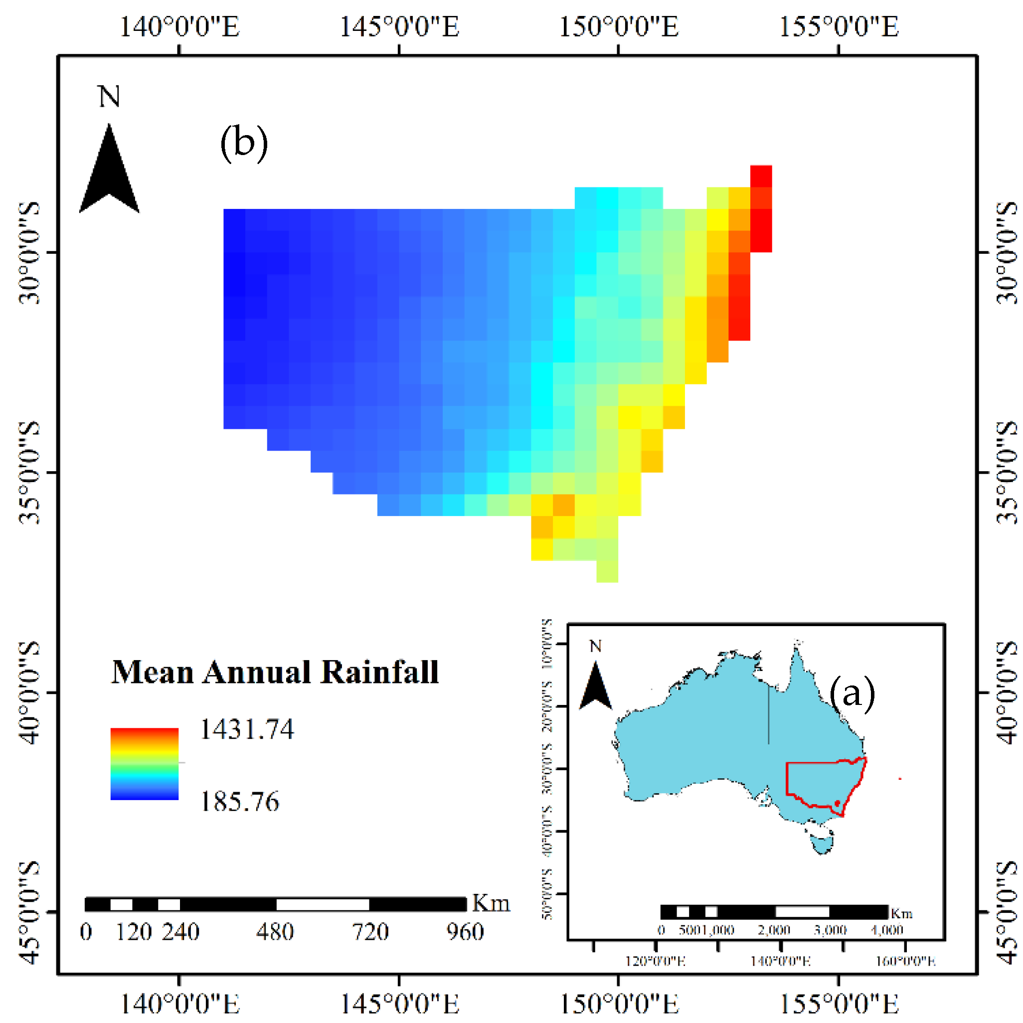
The NSW region (Figure 1) is situated in the south-eastern part of Australia and has experienced three major droughts during the past 125 years (Federation Drought (1895–1902), World War II Drought (1937–1945), and Millennium Drought (2001–2010)) and several minor droughts. The increase in frequent drought occurrences can be attributed to the changes in rainfall and temperature patterns. The effect of climatic drivers on rainfall and their subsequent effect on drought is critical to understand future drought trends. The effect of these drivers arises from the atmospheric–oceanic phenomena in the Pacific Ocean, Indian Ocean, and Southern Ocean. These phenomena, caused by atmospheric pressure anomalies and sea surface temperature (SST) in the Pacific, are known as ENSO and PDO. The determination of the ENSO phase is based on an index, which could be either SST-based or atmosphere-based [40]. At present, the index which best defines the ENSO event is lacking [41]. The SST-based indices affecting NSW region are Nino 3.0, Nino 3.4, and Nino 4.0, and the atmosphere-based index is known as the Southern Oscillation Index (SOI). Similarly, the change of anomalies in the Southern Ocean is known as SAM, and in the Indian Ocean as IOD. Each of these climatic drivers affects rainfall during various seasons of the year; for example, changes in SAM index were responsible for 15% of weekly rainfall during 1979–2005, with little to no contribution in the autumn and spring period [42]. The influence of each of these drivers on rainfall was described in detail by Duc et al. [43].
Data Used
The present study utilizes several meteorological and climatic variables for SPEI forecasting. The meteorological variables were collected from the Climatic Research Unit (CRU) dataset developed by the University of East Anglia at 0.5 × 0.5 m2 spatial resolution from 1901 to 2018 [44]. The spatial distribution of drought forecasting is usually also considered by dividing the area based on various factors such as altitude, climate, and agricultural practices [45]. However, in the present study we focus only on understanding the temporal trend by calculating the mean of meteorological factors for the entire study area. This would provide a basis for determining whether global climatic datasets can be used for forecasting and understanding the factors influencing drought occurrences. The meteorological factors were selected based on variables available in the CRU database and their significance in affecting drought. In addition to the usual factors used for forecasting, such as precipitation, temperature, and potential evapotranspiration, the use of cloud cover for drought studies is often neglected, even though it is significant in understanding the hydrological cycle [46]. Therefore, this study also includes cloud cover as a factor, as well as various climatic indices and sea surface temperature, which are used as regression covariates for the study (Table 1).
3. Methodology
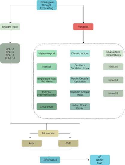
The overall methodological flow chart used in this study is shown in Figure 2. It involves the determination of the drought index at different time scales. Thereafter, the drought index values are forecasted using machine learning approaches (ANN, SVR) utilizing different drought influencing parameters as variables. The results determined using ML models were verified using three different statistical metrics.
3.1. Drought Index Calculation
The drought index used in the present study is SPEI [11,47,48], which is based on rainfall and potential evapotranspiration (PET), and is suited to analysis of the effect of climate change on drought events [10,11] and has gained popularity for drought analysis. The determination of PET was carried out using Hargreave’s method, owing to its simplicity and data availability. Although the Penman–Monteith methodology is recommended as the most suitable method, Hargreave’s method can be used as a substitute if an adequate dataset is unavailable [10]. The index calculation is based on the “climatic water balance” method, which is the difference between precipitation and PET. Thereafter, the summations of the differences are determined at relevant time periods and fitted to a log-logistic probability distribution model. For the study, the R package [49] was used to determine SPEI at time scales of 1, 3, 6, and 12 months. The purpose of determining the index at various time scales was to understand the forecasting capabilities for both short-term and long-term trends. Table 2 shows the drought characterization based on SPEI values.
3.2. Artificial Neural Networks
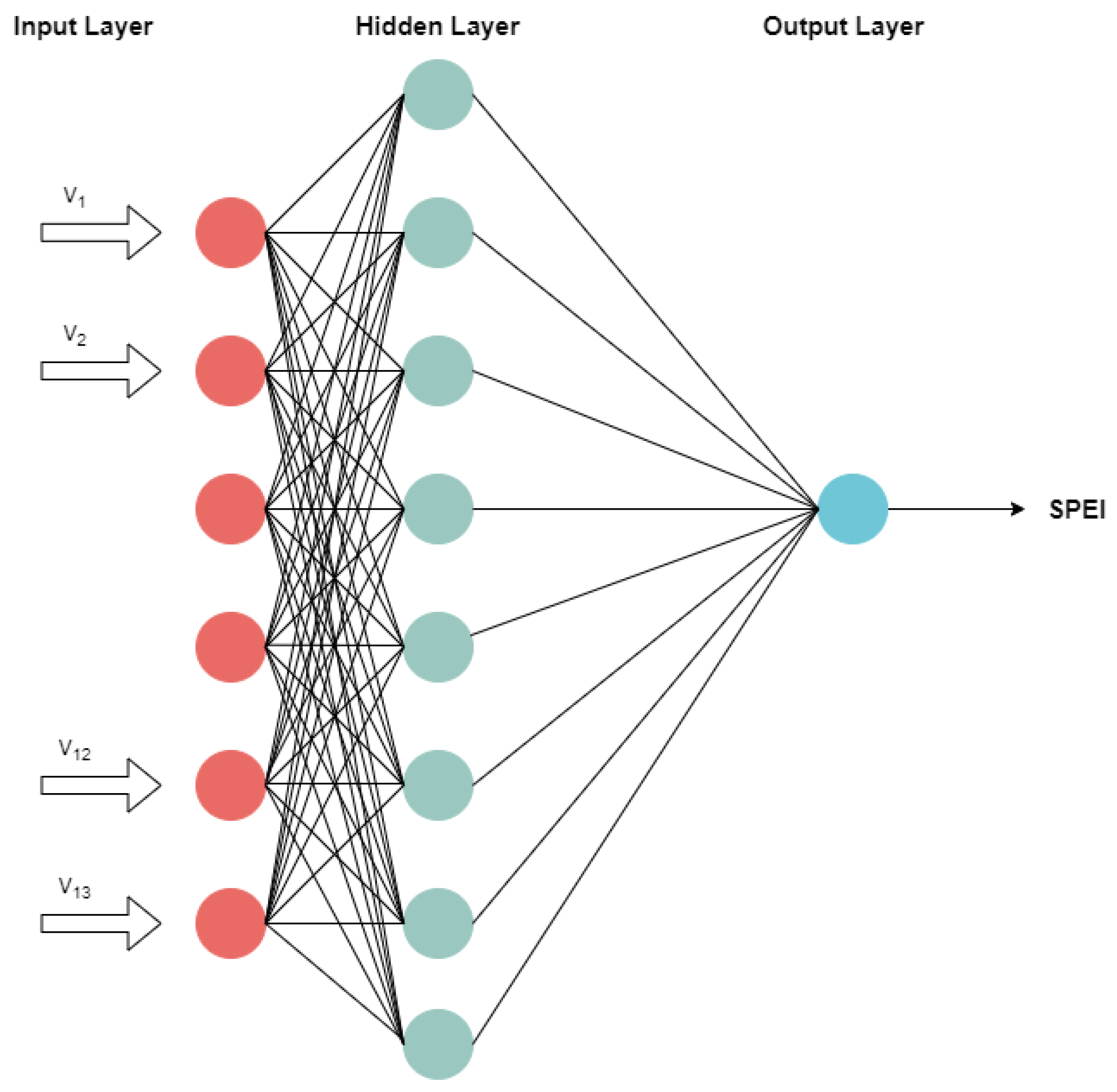
The aim of using an ANN-based model is to determine a relationship between input variables and forecasted future values without any pre-defined programming [18,30]. This makes it ideal for drought forecasting as drought characteristics are stochastic in nature and the understanding of the processes involved is rather complex [50]. There are several types of ANN, of which the multi-layer perceptron (MLP) neural network is one of the most popular models, and consists of an input layer, a single or multiple hidden layers, and an output layer. Figure 3 represents a general architecture of the ANN model, illustrating the signals transmitting through the network layer by layer in a forward direction. The input layer takes in the variables and thereafter the network uses a learning algorithm to determine the best combination of weights producing the least error, also known as training. The hidden layer comprises neuron alike, processing elements connecting the input and output layers.
MLP minimizes the error between the predicted and actual values by updating the weights among every node. The training of MLPs was conducted using the Levenberg–Marquardt (LM) back-propagation algorithm which is based on the steepest gradient descent and the Gauss–Newton iteration method [51,52], and has often been used in hydrologic forecasting because of its simplicity. During the learning process, the weights of the nodes were adjusted based on the error convergence technique with an aim to obtain the desired output for a specific input parameter. Generally, the output layer error propagates backwards to the input layer via the hidden layer to obtain the final output. The weights were determined based on the gradient descent method, which adjusts the interconnected weights with an aim to minimize the output error. The activation function for the hidden layer and output layer were the hyperbolic tangent sigmoid transfer function and linear function, respectively. Another critical issue in the use of an ANN is the determination of the number of hidden neurons and nodes, which is highly significant, especially in hydrological processes due to the nonlinear nature of variables and their interrelationships. Although there is no fixed methodology for determining the number of hidden neurons to be used, reference [53] empirically formulated that log (N), where N is the number of training samples, could provide the best performance. Later, reference [25] found the optimal number of neurons to be 2n + 1, with n being the number of input layers. Therefore, in the present study a trial-and-error approach was used, with the number of hidden neurons to be between log(N) and 2n + 1. Thereafter, the number of neurons that provided the least root-mean-square-error (RMSE) value was selected. In addition to the above-mentioned steps, the input variables were standardized between 0 and 1.
ANN models may suffer from over-fitting. To prevent this an early stopping method, namely generalization loss, was used. Similarly, SVR may suffer from over-fitting and under-fitting during calibration and validation periods, respectively [20]. In such cases, the inputs are mapped at a higher dimension space so that the initial non-linear relationship between the prediction and the variables becomes linear, achieved through a kernel function. This makes it capable of handling smaller datasets and several variables [54]. The selection of the input variables is significant and therefore we aimed to comprehend all of the variables while applying the relevant factors at different time scales to understand drought forecasting.
3.3. Support Vector Regression
Support vector regression (SVR) was developed by [55] to solve prediction problems and is a part of the regression aspect of a support vector machine (SVM). The key difference between SVR and an ANN is that the former aims to minimize generalization error whereas the latter seeks to reduce training error. In addition, unlike ANN, which works on the empirical risk minimization principle, SVR works on the structural risk minimization principle [3]. The use of SVR has been previously conducted for both short-term and long-term drought trends using different kernel types, such as ‘linear’, ‘poly’, and ‘rbf and sigmoid’ [3]. However, the ‘rbf’ kernel type has proved to be effective and was used for the current analysis. In addition to the kernel type, the model is dependent on three different parameters: gamma, cost, and epsilon [1]. The first parameter aims to reduce the model space and complexity, the second parameter reflects capacity control, and the final parameter represents the loss function, which describes the regression vector without all of the input data [56]. The parameter selection was based on a trial-and-error approach, and the combination which produces the least RMSE score was selected.
For the present study, the data was split into a training period (1901–2010) and a testing period (2011–2018) for drought forecasting using both models.
3.4. Performance Metrics
The performance of both models for predicting SPEI was analyzed using different score metrics: (a) coefficient of determination (R2) (Equations (1) and (2)), which measures the correlation degree of the model with the highest value indicating better performance; (b) RMSE (Equations (3) and (4)), which measures the variance of errors independent of sample size; and (c) mean absolute error (MAE) (Equation (5)), which determines the average of absolute errors, analyzing the degree of proximity of forecasted values with the observed values [57,58]. The formulae for these metrics are as follows:
where is the mean value, and are observed and forecasted values, and N is the number of data points.
where SSE refers to sum of squared errors.
4. Results and Discussions
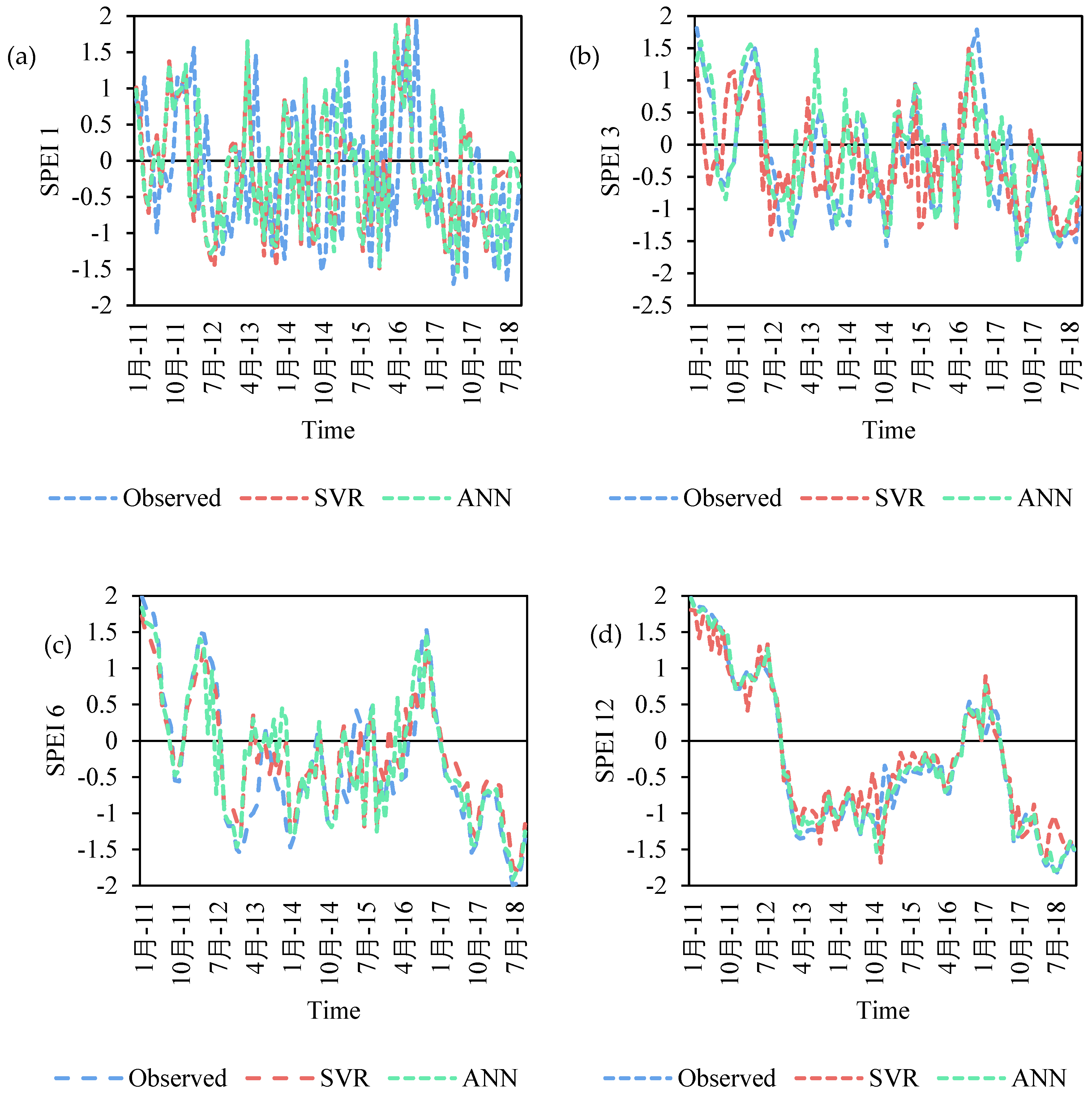
The analysis was performed in the Python environment for both SVR and ANN models. For SVR models, the best parameters for each time scale and the parameters which provided the lowest RMSE and the highest R2 value were selected. Table 3 illustrates the best parameters determined under each SPEI time scale and the corresponding performance metrics. The correlation analysis of the variables and the drought index reveals that at all time scales, the SSTs have a negative correlation, and among the climatic indices PDO had a negative correlation. The results (Figure 4) reveal that higher time scales (12 months) provided better results with R2 value of 0.75 whereas the lower time scales (1 month) had R2 value of 0.61. In terms of understanding the variation in the observed and predicted SPEI values, during the validation period it was observed that for SPEI 12, the SVR model predicted higher values of the drought index (more than 15%) during June 2014–February 2015 and under-predicted during February–July 2012. In the case of SPEI 1 and 3, there are several periods where the index was significantly under-predicted or over-predicted; however, most of these instances occurred during the months of August–December.
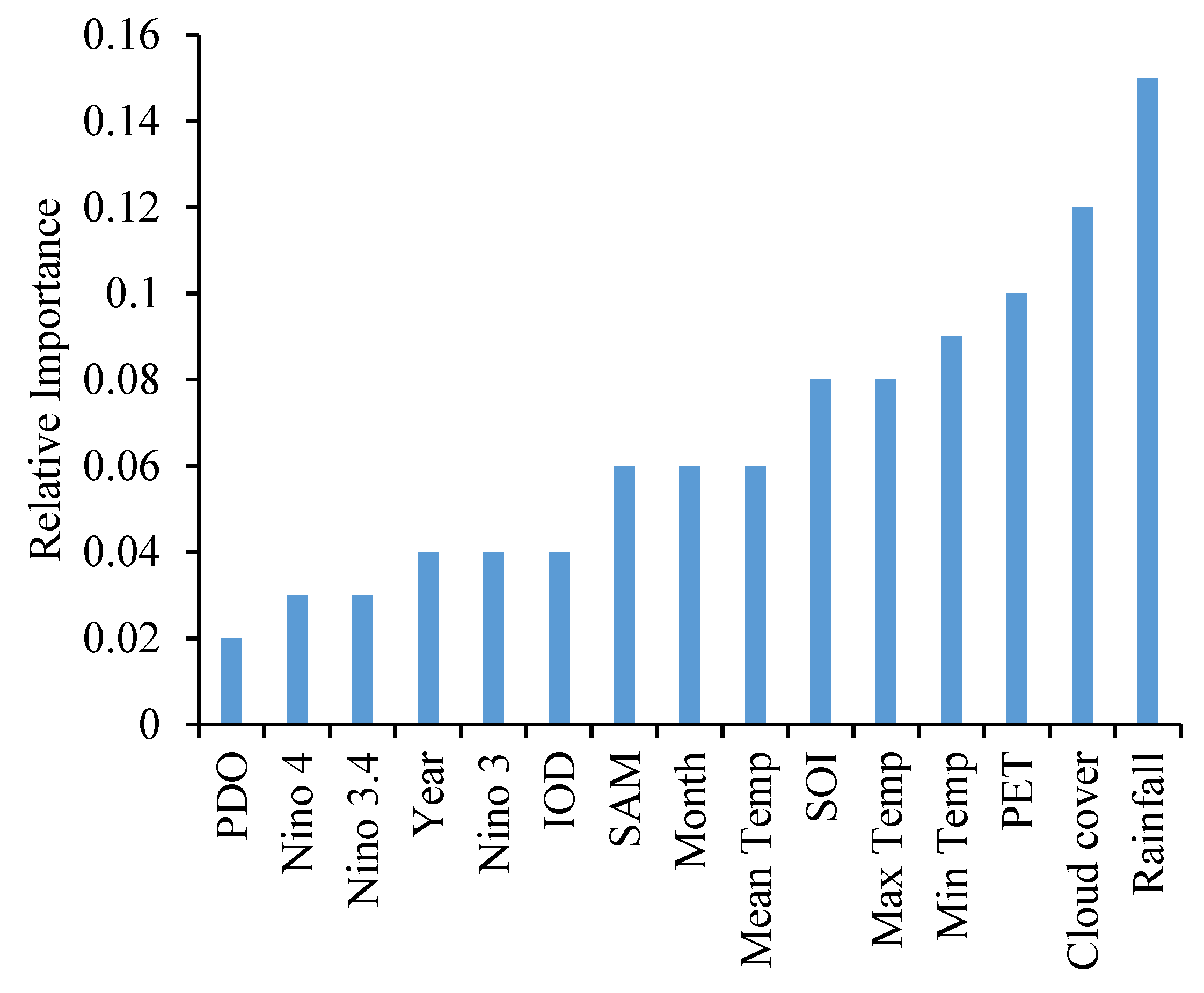
In case of the ANN, the first crucial aspect is to determine the number of hidden neurons, based on the lowest RMSE values using the training dataset. For the present study, the number of hidden neurons was found to be 14 (1 month and 3 months) and 15 (6 months and 12 months). The number of input neurons was determined based on the relative importance of the variables. The relative importance was determined using the ELI5 (https://pypi.org/project/eli5/) Python package, which enables debugging of the classifiers and explaining the predictions. The relative importance of the variables is illustrated in Figure 5. This is significant in determining the variables making the most significant contribution. The results indicate that among the meteorological variables, rainfall, minimum temperature, and cloud cover are important. Similarly, for climatic indices, SOI, and SAM are significant compared to the others, whereas the SSTs had little significance.
Understanding the variation in the forecasting at different durations using the ANN (Table 4) suggests that the model did not show a great amount of difference at 6- and 12-month time scales, with a small number of exceptions. As an example, for the predicted SPEI values at 1- and 3-month time scales, using the ANN, 52.3% of the observed values were over-predicted and 47.7% were under-predicted. Similarly, at longer time scales, 45.2% were under-predicted and 54.2% were over-predicted. The model performance of the ANN model reveals that it was superior to SVR at all of the time scales. The models better predicted SPEI values at 6 and 12 months with R2 values of 0.81 and 0.86, respectively. We also analyzed the variation in the predicted and observed values as per different drought classes (moderate to extreme dry conditions) during the testing period. For SPEI 1, the number of months under moderately dry conditions was 13, under severely dry conditions was 6, and under extreme dry conditions was zero. For severe dry conditions, SVR was able to predict drought earlier or simultaneously, however, it did not detect any severely dry conditions. This suggests that SVR has the capability to determine the onset of short-term moderately dry droughts prior to their actual occurrence, which could be useful for drought mitigation. Similar results were observed for SPEI 3 values. In the case of the ANN, the predicted values also predicted drought onset before the observed values, but it was also able to predict a greater number of drought months and higher intensity. As an example, the observed SPEI 6 values from September 2012 to March 2013 suggested moderately dry and extremely dry conditions, with December and January months belonging to the latter class. The predicted ANN values during the same time period suggested moderate drought conditions from September to January. However, SVR predicted drought for December and January only. A similar observation was made for a time period between May and October 2018, for which the ANN predicted a greater number of drought months compared to SVR. The variation in SPEI 12 values between observed and predicted also yielded similar patterns. Therefore, it can be said that for long-term drought conditions, the ANN has the ability to predict the onset and duration with a certain degree of confidence. For the SVR model, it is sufficient only for onset determination for short-term droughts and the forecasting capability for other drought components, such as duration and intensity, needs to be determined using other neural network approaches.
The study shows that both ANN and SVR are capable of forecasting the temporal drought aspects for NSW, with ANN performing better than SVR. Findings of previous research regarding the relative performance of these two models are contentious. As an example, Lima et al. [59] conducted a study on precipitation forecasts, and found that SVR performs better when MAE is considered as a performance metric and ANN performs better when MSE is considered as a performance metric. Similarly, reference [60] found that both models have comparable performance as the size of training set is increased. The performance of SVR is dependent on the choice of kernel and the associated parameters. This was carried out using a trial-and-error approach, which increased the computation time due to the large dataset size. The uncertainty among the parameters increases the number of trials required to find the optimal model. In the case of the ANN, reliable models can be developed by varying the number of neurons in the hidden layer. In terms of time scales, longer-time scales were better predicted compared to shorter time scales. This could be due to the strong correlation between climatic indices and drought occurrence at longer time scales. Therefore, ANN models can be used as a preliminary step to determine temporal drought forecasts on a regional scale, which could prove to be helpful for policy makers. Future works should look at the development of complex ANN models and deep neural networks which would provide greater insights into forecasting drought and its characteristics in the region.
5. Conclusions
Droughts are a severe and recurring natural hazard, resulting in serious damage to agricultural output and economies. The recent trend of an increase in drought incidence is related to climate change and such incidences are set to increase in the future. This study analyzes the forecasting of temporal drought trends in New South Wales, located in the south-eastern part of Australia. The region has a history of droughts and the influence of climatic drivers is further intensifying drought severity. The present work aims to forecast temporal drought events, using SPEI as a drought indicator, and understand its relationship with several meteorological, climate, and sea surface temperature indices. The data for determining SPEI was gathered from a global climatological dataset, CRU, from which other meteorological factors were also collected. The forecasting of SPEI was conducted using two machine learning algorithms, ANN and SVR. These models were selected based on their overwhelming popularity in data science. In this study, we used these models to study drought events globally and their ability to analyze a non-linear dataset. The study was conducted from 1901–2018, of which 1901–2010 was used as a training period and the remainder as a testing period. Such a study is crucial, as little research has been conducted using data-driven models for NSW to elucidate relevant climatic factors for the analysis. Although this study is lacking in terms of spatial context, it provides deeper understanding from a temporal perspective, and in the use of a global climatological dataset for understanding drought trends under future climate scenarios. The conclusions from the study are as follows:
- The ANN models proved to be significantly better than SVR models at all the time scales studied. In addition, in both cases, forecasting at longer time scales provided better R2 values, suggesting these models be used for long-term forecasting rather than short-term.
- The study used various input variable categories. The relative importance of these variables determined from using the ANN model suggested that sea surface temperatures may not have a significant effect on the temporal aspect of drought as compared to the other meteorological and climatic indices.
- The present study is the first of its kind using a global climatological dataset for NSW. It is likely that future research will increasingly employ such datasets. Further study needs to be conducted on understanding the effect of variables at a spatial scale and in forecasting using more advanced computational approaches.
Author Contributions
Conceptualization, A.D. and B.P.; methodology and formal analysis, A.D.; data curation, A.D.; writing—original draft preparation, A.D.; writing—review and editing, B.P.; supervision, B.P.; funding—B.P. and A.M.A., All authors have read and agreed to the published version of the manuscript.
Funding
This research was supported by the Centre for Advanced Modelling and Geospatial Information Systems (CAMGIS), Faculty of Engineering and IT in the University of Technology Sydney (UTS). This research was also supported by Researchers Supporting Project number RSP-2020/14, King Saud University, Riyadh, Saudi Arabia.
Conflicts of Interest
The authors declare no conflict of interest.
References
- Belayneh, A.; Adamowski, J.; Khalil, B. Short-term SPI drought forecasting in the Awash River Basin in Ethiopia using wavelet transforms and machine learning methods. Sustain. Water Resour. Manag. 2015, 2, 87–101. [Google Scholar] [CrossRef]
- Fung, K.; Huang, Y.; Koo, C.; Soh, Y. Drought forecasting: A review of modelling approaches 2007–2017. J. Water Clim. Chang. 2019, 1–29. [Google Scholar] [CrossRef]
- Belayneh, A.; Adamowski, J.; Khalil, B.; Ozga-Zielinski, B. Long-term SPI drought forecasting in the Awash River Basin in Ethiopia using wavelet neural network and wavelet support vector regression models. J. Hydrol. 2014, 508, 418–429. [Google Scholar] [CrossRef]
- Mishra, A.; Singh, V.P. A review of drought concepts. J. Hydrol. 2010, 391, 202–216. [Google Scholar] [CrossRef]
- Cancelliere, A.; Di Mauro, G.; Bonaccorso, B.; Rossi, G. Drought forecasting using the Standardized Precipitation Index. Water Resour. Manag. 2006, 21, 801–819. [Google Scholar] [CrossRef]
- Rossi, G.; Vega, T.; Bonaccorso, B. Methods and Tools for Drought Analysis and Management; Springer Science & Business Media: Berlin, Germany, 2007; Volume 62. [Google Scholar]
- Sheffield, J.; Wood, E.F. Drought: Past Problems and Future Scenarios; Routledge: Abingdon, UK, 2012. [Google Scholar]
- Yihdego, Y.; Vaheddoost, B.; Al-Weshah, R.A. Drought indices and indicators revisited. Arab. J. Geosci. 2019, 12, 69. [Google Scholar] [CrossRef]
- McKee, T.B.; Doesken, N.J.; Kleist, J. The relationship of drought frequency and duration to time scales. In Proceedings of the 8th Conference on Applied Climatology, Anaheim, CA, USA, January 1993; pp. 179–184. [Google Scholar]
- Beguería, S.; Vicente-Serrano, S.; Reig, F.; Latorre, B. Standardized precipitation evapotranspiration index (SPEI) revisited: Parameter fitting, evapotranspiration models, tools, datasets and drought monitoring. Int. J. Clim. 2013, 34, 3001–3023. [Google Scholar] [CrossRef] [Green Version]
- Vicente-Serrano, S.; Beguería, S.; I López-Moreno, J. A Multiscalar Drought Index Sensitive to Global Warming: The Standardized Precipitation Evapotranspiration Index. J. Clim. 2010, 23, 1696–1718. [Google Scholar] [CrossRef] [Green Version]
- Manzano, A.; Clemente, M.A.; Morata, A.; Luna, M.Y.; Beguería, S.; Vicente-Serrano, S.M.; Martín, M.L. Analysis of the atmospheric circulation pattern effects over SPEI drought index in Spain. Atmos. Res. 2019, 230, 104630. [Google Scholar] [CrossRef]
- Hao, Z.; Singh, V.P.; Xia, Y. Seasonal Drought Prediction: Advances, Challenges, and Future Prospects. Rev. Geophys. 2018, 56, 108–141. [Google Scholar] [CrossRef] [Green Version]
- Ma, F.; Luo, L.; Ye, A.; Duan, Q. Seasonal drought predictability and forecast skill in the semi-arid endorheic Heihe River basin in northwestern China. Hydrol. Earth Syst. Sci. 2018, 22, 5697–5709. [Google Scholar] [CrossRef] [Green Version]
- Hudson, D.; Alves, O.; Hendon, H.H.; Marshall, A.G. Bridging the gap between weather and seasonal forecasting: Intraseasonal forecasting for Australia. Q. J. R. Meteorol. Soc. 2011, 137, 673–689. [Google Scholar] [CrossRef]
- Dikshit, A.; Sarkar, R.; Pradhan, B.; Segoni, S.; Alamri, A.M. Rainfall Induced Landslide Studies in Indian Himalayan Region: A Critical Review. Appl. Sci. 2020, 10, 2466. [Google Scholar] [CrossRef] [Green Version]
- Deo, R.C.; Şahin, M. Application of the Artificial Neural Network model for prediction of monthly Standardized Precipitation and Evapotranspiration Index using hydrometeorological parameters and climate indices in eastern Australia. Atmos. Res. 2015, 161, 65–81. [Google Scholar] [CrossRef]
- Bishop, C.M. Pattern Recognition and Machine Learning; Springer: Berlin/Heidelberg, Germany, 2006. [Google Scholar]
- Sachindra, D.A.; Kanae, S. Machine learning for downscaling: The use of parallel multiple populations in genetic programming. Stoch. Environ. Res. Risk Assess. 2019, 33, 1497–1533. [Google Scholar] [CrossRef] [Green Version]
- Khan, N.; Sachindra, D.; Shahid, S.; Ahmed, K.; Shiru, M.S.; Nawaz, N. Prediction of droughts over Pakistan using machine learning algorithms. Adv. Water Resour. 2020, 139, 103562. [Google Scholar] [CrossRef]
- Feng, P.; Wang, B.; Liu, D.L.; Yu, Q. Machine learning-based integration of remotely-sensed drought factors can improve the estimation of agricultural drought in South-Eastern Australia. Agric. Syst. 2019, 173, 303–316. [Google Scholar] [CrossRef]
- Ortiz-Garcia, E.; Salcedo-Sanz, S.; Casanova-Mateo, C. Accurate precipitation prediction with support vector classifiers: A study including novel predictive variables and observational data. Atmos. Res. 2014, 139, 128–136. [Google Scholar] [CrossRef]
- Mishra, A.K.; Desai, V.R.; Singh, V.P. Drought Forecasting Using a Hybrid Stochastic and Neural Network Model. J. Hydrol. Eng. 2007, 12, 626–638. [Google Scholar] [CrossRef]
- Haidary, A.; Amiri, B.J.; Adamowski, J.; Fohrer, N.; Nakane, K. Assessing the Impacts of Four Land Use Types on the Water Quality of Wetlands in Japan. Water Resour. Manag. 2013, 27, 2217–2229. [Google Scholar] [CrossRef]
- Mishra, A.K.; Desai, V. Drought forecasting using feed-forward recursive neural network. Ecol. Model. 2006, 198, 127–138. [Google Scholar] [CrossRef]
- Morid, S.; Smakhtin, V.; Bagherzadeh, K. Drought forecasting using artificial neural networks and time series of drought indices. Int. J. Clim. 2007, 27, 2103–2111. [Google Scholar] [CrossRef]
- Barua, S.; Ng, A.; Perera, C. Artificial Neural Network–Based Drought Forecasting Using a Nonlinear Aggregated Drought Index. J. Hydrol. Eng. 2012, 17, 1408–1413. [Google Scholar] [CrossRef]
- Marj, A.F.; Meijerink, A.M.J. Agricultural drought forecasting using satellite images, climate indices and artificial neural network. Int. J. Remote Sens. 2011, 32, 9707–9719. [Google Scholar] [CrossRef]
- Xiang, B.; Lin, S.J.; Zhao, M.; Johnson, N.C.; Yang, X.; Jiang, X. Subseasonal week 3–5 surface air temperature prediction during boreal wintertime in a GFDL model. Geophys. Res. Lett. 2019, 46, 416–425. [Google Scholar] [CrossRef] [Green Version]
- Santos, J.; Silva, M.C.; Pulido-Calvo, I. Spring drought prediction based on winter NAO and global SST in Portugal. Hydrol. Process. 2012, 28, 1009–1024. [Google Scholar] [CrossRef]
- Ganguli, P.; Reddy, M.J. Ensemble prediction of regional droughts using climate inputs and the SVM–copula approach. Hydrol. Process. 2013, 28, 4989–5009. [Google Scholar] [CrossRef]
- Dey, R.; Lewis, S.C.; Arblaster, J.; Abram, N.J. A review of past and projected changes in Australia’s rainfall. Wiley Interdiscip. Rev. Clim. Chang. 2019, 10, e577. [Google Scholar] [CrossRef]
- Hope, P.; Timbal, B.; Fawcett, R. Associations between rainfall variability in the southwest and southeast of Australia and their evolution through time. Int. J. Clim. 2009, 30, 1360–1371. [Google Scholar] [CrossRef]
- Timbal, B.; Arblaster, J.; Braganza, K.; Fernandez, E.; Hendon, H.; Murphy, B.; Raupach, M.; Rakich, C.; Smith, I.; Whan, K. Understanding the Anthropogenic Nature of the Observed Rainfall Decline across South Eastern Australia. Available online: https://www.cawcr.gov.au/technical-reports/CTR_026.pdf (accessed on 30 April 2020).
- Verdon-Kidd, D.C.; Kiem, A.S. Nature and causes of protracted droughts in southeast Australia: Comparison between the Federation, WWII, and Big Dry droughts. Geophys. Res. Lett. 2009, 36, 36. [Google Scholar] [CrossRef]
- Trenberth, K.E.; Dai, A.; Van Der Schrier, G.; Jones, P.; Barichivich, J.; Briffa, K.R.; Sheffield, J. Global warming and changes in drought. Nat. Clim. Chang. 2013, 4, 17–22. [Google Scholar] [CrossRef]
- Cai, W.; Van Rensch, P.; Cowan, T.; Hendon, H.H. Teleconnection Pathways of ENSO and the IOD and the Mechanisms for Impacts on Australian Rainfall. J. Clim. 2011, 24, 3910–3923. [Google Scholar] [CrossRef]
- Meneghini, B.; Simmonds, I.H.; Smith, I.N. Association between Australian rainfall and the Southern Annular Mode. Int. J. Clim. 2006, 27, 109–121. [Google Scholar] [CrossRef]
- Latif, M.; Kleeman, R.; Eckert, C. Greenhouse Warming, Decadal Variability, or El Niño? An Attempt to Understand the Anomalous 1990s. J. Clim. 1997, 10, 2221–2239. [Google Scholar] [CrossRef] [Green Version]
- Hanley, D.E.; Bourassa, M.; O’Brien, J.J.; Smith, S.; Spade, E.R. A Quantitative Evaluation of ENSO Indices. J. Clim. 2003, 16, 1249–1258. [Google Scholar] [CrossRef]
- Huang, B.; L’Heureux, M.L.; Lawrimore, J.; Liu, C.; Zhang, H.-M.; Banzon, V.; Hu, Z.; Kumar, A. Why Did Large Differences Arise in the Sea Surface Temperature Datasets across the Tropical Pacific during 2012? J. Atmos. Ocean. Technol. 2013, 30, 2944–2953. [Google Scholar] [CrossRef]
- Hendon, H.H.; Thompson, D.W.J.; Wheeler, M. Australian Rainfall and Surface Temperature Variations Associated with the Southern Hemisphere Annular Mode. J. Clim. 2007, 20, 2452–2467. [Google Scholar] [CrossRef]
- Duc, H.N.; Rivett, K.; Macsween, K.; Le-Anh, L. Association of climate drivers with rainfall in New South Wales, Australia, using Bayesian Model Averaging. Theor. Appl. Clim. 2015, 127, 169–185. [Google Scholar] [CrossRef]
- Harris, I.; Osborn, T.J.; Jones, P.; Lister, D. Version 4 of the CRU TS monthly high-resolution gridded multivariate climate dataset. Sci. Data 2020, 7, 109–118. [Google Scholar] [CrossRef] [Green Version]
- Rim, C.-S. The implications of geography and climate on drought trend. Int. J. Clim. 2012, 33, 2799–2815. [Google Scholar] [CrossRef]
- Martins, V.S.; Novo, E.; Lyapustin, A.; Aragão, L.E.; Freitas, S.R.; Barbosa, C.C.F. Seasonal and interannual assessment of cloud cover and atmospheric constituents across the Amazon (2000–2015): Insights for remote sensing and climate analysis. ISPRS J. Photogramm. Remote Sens. 2018, 145, 309–327. [Google Scholar] [CrossRef] [Green Version]
- Vicente-Serrano, S.; Azorin-Molina, C.; Sanchez-Lorenzo, A.; Revuelto, J.; I López-Moreno, J.; Gonzalez-Hidalgo, J.C.; Morán-Tejeda, E.; Espejo, F. Reference evapotranspiration variability and trends in Spain, 1961–2011. Glob. Planet. Chang. 2014, 121, 26–40. [Google Scholar] [CrossRef] [Green Version]
- Vicente-Serrano, S.; Beguería, S.; Lorenzo-Lacruz, J.; Camarero, J.J.; I López-Moreno, J.; Azorin-Molina, C.; Revuelto, J.; Morán-Tejeda, E.; Sanchez-Lorenzo, A. Performance of Drought Indices for Ecological, Agricultural, and Hydrological Applications. Earth Interact. 2012, 16, 1–27. [Google Scholar] [CrossRef] [Green Version]
- Beguería, S.; Vicente-Serrano, S.M.; Beguería, M.S. Package ‘SPEI’. 2017. Available online: https://cran.r-project.org/web/packages/SPEI/SPEI.pdf (accessed on 30 April 2020).
- Mishra, A.K.; Desai, V.R. Drought forecasting using stochastic models. Stoch. Environ. Res. Risk Assess. 2005, 19, 326–339. [Google Scholar] [CrossRef]
- Hagan, M.; Menhaj, M. Training feedforward networks with the Marquardt algorithm. IEEE Trans. Neural Netw. 1994, 5, 989–993. [Google Scholar] [CrossRef] [PubMed]
- Yu, H.; Wilamowski, B.M. Levenberg-marquardt training. Ind. Electron. Handb. 2011, 5, 1. [Google Scholar]
- Wanas, N.; Auda, G.; Kamel, M.S.; Karray, F. On the optimal number of hidden nodes in a neural network. In Proceedings of the IEEE Canadian Conference on Electrical and Computer Engineering (Cat. No. 98TH8341), Vancouver, BC, Canada, 24–28 May 1998; pp. 918–921. [Google Scholar]
- Bourdin, D.R.; Fleming, S.W.; Stull, R.B. Streamflow Modelling: A Primer on Applications, Approaches and Challenges. Atmos. Ocean 2012, 50, 507–536. [Google Scholar] [CrossRef] [Green Version]
- Vapnik, V. The Nature of Statistical Learning Theory; Springer Science & Business Media: Berlin, Germany, 2013. [Google Scholar]
- Kisi, O.; Çimen, M. A wavelet-support vector machine conjunction model for monthly streamflow forecasting. J. Hydrol. 2011, 399, 132–140. [Google Scholar] [CrossRef]
- Paulescu, M.; Paulescu, E.; Stefu, N. A temperature-based model for global solar irradiance and its application to estimate daily irradiation values. Int. J. Energy Res. 2011, 35, 520–529. [Google Scholar] [CrossRef]
- Tiwari, M.K.; Chatterjee, C. Development of an accurate and reliable hourly flood forecasting model using wavelet–bootstrap–ANN (WBANN) hybrid approach. J. Hydrol. 2010, 394, 458–470. [Google Scholar] [CrossRef]
- Lima, A.R.; Cannon, A.J.; Hsieh, W.W. Nonlinear regression in environmental sciences by support vector machines combined with evolutionary strategy. Comput. Geosci. 2013, 50, 136–144. [Google Scholar] [CrossRef]
- Chevalier, R.F.; Hoogenboom, G.; McClendon, R.W.; Paz, J.O. Support vector regression with reduced training sets for air temperature prediction: A comparison with artificial neural networks. Neural Comput. Appl. 2010, 20, 151–159. [Google Scholar] [CrossRef]
Figure 1.
(a) Study area in Australia, and (b) mean annual rainfall of NSW (1901–2018) based on Climatic Research Unit–Time Series (CRU - TS) dataset.
Figure 1.
(a) Study area in Australia, and (b) mean annual rainfall of NSW (1901–2018) based on Climatic Research Unit–Time Series (CRU - TS) dataset.

Figure 2.
Methodological framework of the study conducted.

Figure 3.
General architecture of an artificial neural network (ANN) model.

Figure 4.
Variation in SPEI values at different time scales (a) 1 month; (b) 3 months; (c) 6 months; (d) 12 months between observed and predicted values using SVR and RNN.
Figure 4.
Variation in SPEI values at different time scales (a) 1 month; (b) 3 months; (c) 6 months; (d) 12 months between observed and predicted values using SVR and RNN.

Figure 5.
Relative importance plot of the variables for the ANN model.


Table 1.
Input parameters used for drought forecasting.
| Meteorological Factors | Climatic Indices | Sea Surface Temperature |
|---|---|---|
| Monthly mean precipitation | Southern Oscillation Index | Nino 3.4 SST (5° N–5° S,170° W–120° W) |
| Monthly mean air temperature | Pacific Decadal Oscillation | Nino 4.0 SST (5° N–5° S, 160° E–150° W) |
| Monthly maximum air temperature | Southern Annular Mode | Nino 3.0 SST (5° N–5° S,150° W–90° W) |
| Monthly minimum air temperature | Indian Ocean Dipole | |
| Potential evapotranspiration | ||
| Cloud cover |
Table 2.
Drought classification according to Standard Precipitation Evaporation Index (SPEI) definition.
Table 2.
Drought classification according to Standard Precipitation Evaporation Index (SPEI) definition.
| SPEI Classifications | Categories |
|---|---|
| ≤−2.0 | Extremely Dry |
| −1.99 to −1.5 | Severely Dry |
| −1.49 to −1.0 | Moderately Dry |
| −0.99 to 0.99 | Near Normal |
| 1.0 to 1.49 | Moderately Wet |
| 1.5 to 1.99 | Severely Wet |
| ≥2.0 | Extremely Wet |
Table 3.
Model performance of various SPEI time scales for support vector regression (SVR) models.
| Prediction | R2 | RMSE | MAE |
|---|---|---|---|
| SPEI 1 | 0.61 | 0.94 | 0.93 |
| SPEI 3 | 0.72 | 0.68 | 0.65 |
| SPEI 6 | 0.74 | 0.62 | 0.59 |
| SPEI 12 | 0.75 | 0.58 | 0.55 |
Table 4.
Model performance under ANN models.
| Prediction | R2 | RMSE | MAE |
|---|---|---|---|
| SPEI 1 | 0.72 | 0.68 | 0.65 |
| SPEI 3 | 0.75 | 0.62 | 0.59 |
| SPEI 6 | 0.81 | 0.54 | 0.51 |
| SPEI 12 | 0.86 | 0.24 | 0.23 |
© 2020 by the authors. Licensee MDPI, Basel, Switzerland. This article is an open access article distributed under the terms and conditions of the Creative Commons Attribution (CC BY) license (http://creativecommons.org/licenses/by/4.0/).
Share and Cite
MDPI and ACS Style
Dikshit, A.; Pradhan, B.; Alamri, A.M. Temporal Hydrological Drought Index Forecasting for New South Wales, Australia Using Machine Learning Approaches. Atmosphere 2020, 11, 585. https://0-doi-org.brum.beds.ac.uk/10.3390/atmos11060585
AMA Style
Dikshit A, Pradhan B, Alamri AM. Temporal Hydrological Drought Index Forecasting for New South Wales, Australia Using Machine Learning Approaches. Atmosphere. 2020; 11(6):585. https://0-doi-org.brum.beds.ac.uk/10.3390/atmos11060585
Chicago/Turabian StyleDikshit, Abhirup, Biswajeet Pradhan, and Abdullah M. Alamri. 2020. "Temporal Hydrological Drought Index Forecasting for New South Wales, Australia Using Machine Learning Approaches" Atmosphere 11, no. 6: 585. https://0-doi-org.brum.beds.ac.uk/10.3390/atmos11060585
Note that from the first issue of 2016, this journal uses article numbers instead of page numbers. See further details here.