Article

Validation of the Atmospheric Boundary Layer Height Estimated from the MODIS Atmospheric Profile Data at an Equatorial Site

1
Faculty of Science, Mbarara University of Science and Technology, Mbarara, Uganda
2
Department of Physics, Muni University, Arua, Uganda
3
Department of Physics and Astronomy, Colgate University, Hamilton, NY 13346, USA
*
Author to whom correspondence should be addressed.
Submission received: 1 July 2020 / Revised: 18 August 2020 / Accepted: 24 August 2020 / Published: 26 August 2020
(This article belongs to the Special Issue Regional Air Quality Modeling)

Abstract

:
The atmospheric boundary layer height is important for constraining air pollution and meteorological models. This study attempted to validate the MODIS-estimated atmospheric boundary layer height (ABLH), and variation in the ABLH in Uganda was evaluated. The ABLH was estimated from MODIS data using the mixing ratio profile gradient method and compared to the ABLH estimated from radiosonde data using three different methods. Unlike in studies in other regions of the world, correlations between ABLH estimated using MODIS and radiosonde data were weak, implying limited usefulness of MODIS data for determining ABLH. However, the diurnal variation in MODIS-derived ABLH and particulate matter (PM10) was consistent with the expected inverse relationship between PM10 mass concentration and ABLH, and the mean MODIS-derived ABLH values were significantly lower during wet seasons than dry seasons, as expected.

1. Introduction

The atmospheric boundary layer height (ABLH) is an important parameter for modeling ground-level particulate matter (PM) concentration [1,2,3,4] and meteorological variations [5,6,7]. In the atmospheric boundary layer (ABL), turbulence results due to the diurnal cycle of surface heating and cooling caused by radiant heat flux (among other factors) [7,8,9]. The ABLH marks the top of the layer of the troposphere that is influenced by Earth’s surface and constrains the volume available for mixing in the lower troposphere. Therefore, its variation has been reported to influence numerous atmospheric processes including turbulent heat flux, weather changes, and the dispersion, mixing, scavenging, and deposition of air pollutants [3,7,10]. Its climatology is important for understanding and modeling atmospheric processes.
The ABLH is estimated using atmospheric profiles that are derived from observations made by instruments such as radiosonde, lidar, ceilometers, and other space-based instruments [11,12,13]. Observations are obtained from field campaigns, regular periodic measurements at various stations worldwide, and remote observations [11,12,14]. The most common source of atmospheric profiles is regular periodic measurement using the radiosonde at defined stations worldwide. The radiosonde atmospheric profiles provide good estimates of the ABLH [12,15,16]. However, radiosonde measurements are limited in both spatial and temporal coverage. In East Africa, radiosonde releases are done once or twice per day; in some instances many days are skipped; and in recent years only three stations have been operational in the entire area [17]. These operational stations have significant gaps in coverage; for example, at Entebbe, there were 78 daytime soundings in 2013; 35 in 2014; none in 2015–2017; 34 in 2018; and no more through the current date. The limited spatial and temporal coverage of radiosonde data hampers the possibility of evaluating the diurnal and spatial variation of the boundary layer and its application to air quality and meteorological modeling.
A possible alternative to the radiosonde atmospheric profile data is the moderate resolution spectroradiometer (MODIS) atmospheric profile data [18,19]. MODIS instruments are on board two satellites, Terra and Aqua, that have a morning and early afternoon equator crossing time and are capable of providing nighttime atmospheric profiles. The instrument’s wide swath makes it capable of providing nearly daily global coverage [19,20]. MODIS atmospheric profile data have been used to estimate ABLH in the Heihe river basin and a moderate correlation between the MODIS and Radiosonde ABLH estimates was reported [18].
Due to the possibility that MODIS could significantly enhance the quantification of the ABLH as was seen in Reference [18], this paper attempted to validate the MODIS-estimated ABLH using radiosonde data, determine its relationship with PM10 at selected sites, and evaluate the temporal variations in the ABLH in Uganda (both daily and seasonal). The study provides for the first time a long-term evaluation of the possibility of using MODIS atmospheric profiles for estimating ABLH in an equatorial region.

2. Study Area and Data Sources

This study was done in Uganda, in equatorial East Africa. As described below, radiosonde data was available only at Entebbe Airport; PM10 data were used from three locations; and seasonal variation in MODIS data were analyzed in fourteen climatic zones in Uganda.

2.1. Radiosonde Data

Radiosonde data for all six stations in Uganda were obtained from the IGRA version 2, available at (https://www1.ncdc.noaa.gov/pub/data/igra/). Five stations have been inactive since 1977; only Entebbe Airport had measurements since then; and those measurements end in 2018. Entebbe Airport (reference UGM00063705) is located about 45 km south of Kampala, the capital of Uganda, on a peninsular in Lake Victoria, at latitude 0.05° N, longitude 32.45° E, and altitude 1155 m above sea level. Profile data from this radiosonde station were used to validate the MODIS-estimated ABLH. Radiosonde data were available for some periods of 2013, 2014, and 2018. The atmospheric profile data that were used include profiles of temperature, wind speed, relative humidity, potential temperature, and virtual potential temperature, along with gradients of these variables.

2.2. PM10 Data

PM10 data were collected from three sites with a real-time monitor (TSI SidePak AM510) using an impactor with a 10 μm cut-off, as described in [21]. The sites were in Mbarara, Rubindi, and Kyebando. The sampling site in Mbarara was in the Town Campus of Mbarara University of Science and Technology, where the terrain is relatively flat and open. Rubindi is a hilly rural trading center along the Mbarara-Ibanda road. Kyebando is a relatively hilly region of Kampala with dense housing and businesses. The continuous PM10 data were averaged for the morning (10:00–10:59 a.m.) and afternoon (1:00–1:59 p.m.) LST. This time corresponds to about ±30 min of the satellite overpass time. The time of averaging was chosen in order to co-locate the satellite observation with the ground-based measurement.

2.3. MODIS Data

MODIS sensors on board Terra and Aqua satellites have been observing the Earth since 1999 and 2002, respectively. The two satellites cross the equator at about 10:30 a.m. and 1:30 p.m. local standard time (LST) for Terra and Aqua, respectively. The early afternoon equator crossing enables retrieval of data useful for comparison with radiosonde data. MODIS level 2 atmospheric products MYD07 (Aqua) and MOD07 (Terra) were obtained from the Level-1 and Atmosphere Archive and Distribution System Distributed Active Archive Center (LAADS DAAC) available at (https://modis-atmos.gsfc.nasa.gov/products/atm-profile). Level 2 atmospheric profile data represent five-minute satellite exposure times on 5 × 5 km pixel retrievals. Daytime observations were used due to the fact that at night, ground level temperature inversions occur frequently due to surface cooling. Under conditions of ground level temperature inversion, the methods selected for use in this study are not applicable [9].
MODIS data for Uganda from 28 to 36° E longitude and −1.5 to 5° N latitude were obtained for six years from 2013 to 2018. The level 2 data include geo-location data and height, temperature, and mixing ratio profiles for 20 pressure levels. The mixing ratio profiles were retrieved from the downloaded data on 0.25 by 0.25° (25 by 25 km) grids centered at each selected reference point. The twenty-five km grids aid co-location with ground level observation [22], allow for air mass movement over the location, and provide sufficient time for satellite observation given that each 5 by 5 km grid are five-min observations [23].
Since the average elevation of Uganda is about 1100 m, 850 hPa is normally the lowest available level. For credible analysis and application of MODIS data, the data availability should be greater or equal to 30% [23]. Figure A1 in Appendix A shows the spatial availability of the MODIS estimated ABLH. At all locations data were available more than 30% of the time.
The seasonal variation of ABLH was studied with MODIS data after first classifying the country on the basis of rainfall climatic zones. Climate zoning was chosen because precipitation events have been reported to cause surface cooling that influences the evolution of the ABL [11,24]. Based on the amount and variation of rainfall, Uganda can be divided into fourteen climatic zones, as shown in Figure 1 [25,26].
To evaluate seasonal variation, single point locations were selected from each of the fourteen zones shown in Figure 1. The points selected as the reference for data retrieval are presented in the Appendix A, Table A1. All reference points were selected at urban centers. The place names used are those of the districts where reference points are located. While there was variation in the ABLH between rainfall zones, it was found that the data from all zones followed very similar seasonal trends. In order to present results compactly, only the values averaged over the different zones have been included in this paper.

3. Methods

3.1. Determination of ABLH

The Earth’s daily diurnal cycle of radiative heating and cooling causes heat fluxes between the land and air. These heat fluxes cause modifications of the atmospheric boundary layer (ABL), the bottom layer of the troposphere. Above the ABL is the free atmosphere where air is (in general) unmodified by turbulence.
In this paper, the ABLH was determined using a number of methods described in Reference [9], focusing on convective boundary layers that are typically present in the afternoons. The first set of methods use temperature profiles. The ABLH can be considered as the height at which the potential temperature gradient is a maximum. (Potential temperature is the temperature that a gas parcel would reach if it were adiabatically brought to a standard reference pressure.) A second method of estimating the ABLH, the parcel method, uses the virtual potential temperature, which corrects for both humidity and pressure, and is the potential temperature of dry air that would have the same density as the actual parcel of humid air. At the bottom of the temperature inversion, the virtual potential temperature of a parcel of air is equal to the virtual potential temperature at the surface [9]. Therefore, the parcel method determines the ABLH as the height at which the virtual potential temperature of an air parcel is equal to the virtual potential temperature at the surface. The height obtained using the parcel method is referred to as the mixing height and it is preferred for air quality studies [9].
Water vapour measurements can also be used to estimate the ABLH. Due to turbulent vertical mixing, pollutants, water vapour, and air are assumed to be uniformly mixed within the boundary layer [24]. An abrupt change in the amount of water vapour is expected at the top of the ABL, resulting in a minimum gradient. When parameters that measure the amount of water vapour in the atmosphere (relative humidity and mixing ratio) are considered, the ABLH is computed as the height at which the gradient of such a parameter is minimum.
In this study, the parcel method and two gradient methods (relative humidity and potential temperature) were used for the radiosonde data. The mixing ratio was used for the MODIS data, since that was the method that was found to be successful in [18]. At Entebbe, the radiosonde release is done at about 12:00 LST when surface-based inversions are very unlikely [8,9]. Evidence for surface-based inversions was seen on two days, and these days were excluded from the analysis. The two radiosonde gradient methods were compared to each other in order to illustrate possible differences in ABLH induced by choice of the method [9]. To avoid mistaking variations in the free atmosphere as occurring in the ABL, only heights less than 4000 m above ground level were considered [3,9,14,18].

3.2. Validation of MODIS ABLH

The method of obtaining the ABLH from MODIS data was validated by comparing MODIS-derived ABLH values to ones obtained from radiosonde data. Since the only recent radiosonde data are from Entebbe Airport and are obtained at 12:00 LST, we used the MODIS data from the Aqua satellite, which passes over the ground station at about 1:30 p.m. LST, when a surface-based temperature inversion is unlikely. Due to the possible rapid variations in the atmosphere, the comparison was made only when the satellite overpass time was within 1.5 h of the radiosonde release time. The MODIS-derived ABLH was also compared to PM10 measurements made at three sites in Uganda. Both the morning and afternoon MODIS data were used for this comparison to PM10 measurements.

3.3. Temporal Variation

The six-year MODIS atmospheric products data for both the Aqua and Terra satellites were used to estimate the ABLH for 14 sites selected based on rainfall patterns. Both satellites were used to determine differences between morning and afternoon ABLH values. The grid co-ordinate reference point for the rainfall zones is presented in Table A1. The height of the ABL above ground level was computed. Seasonal trends in the estimated ABLH were investigated by comparing the wet and dry season monthly mean ABLH values.

4. Results

An illustration of the use of the gradient method to estimate the ABLH from profile data is presented in Figure 2, which shows profiles for twelve dates at Entebbe Airport (the dates selected are the first date from months in which valid data existed). These data illustrate the difficulty of using these methods to locate the ABLH. Relatively good correlations are seen between the two radiosonde-based gradient methods (potential temperature and relative humidity) but a poor correlation is seen with the MODIS-based mixing ratio. Some dates show striking differences between the values found using different methods. For example, 1 October 2014, finds the ABLH at approximately 4000 m using relative humidity; 200 m using potential temperatures; and 2000 m using the mixing ratio. On this date, there may have been a cloud between 500 and 3000 m, and the potential temperature method classifies cloud base as the ABLH. The large differences observed on 23 March 2018, may also be due to clouds. Unfortunately, cloud observations were not recorded at this station.

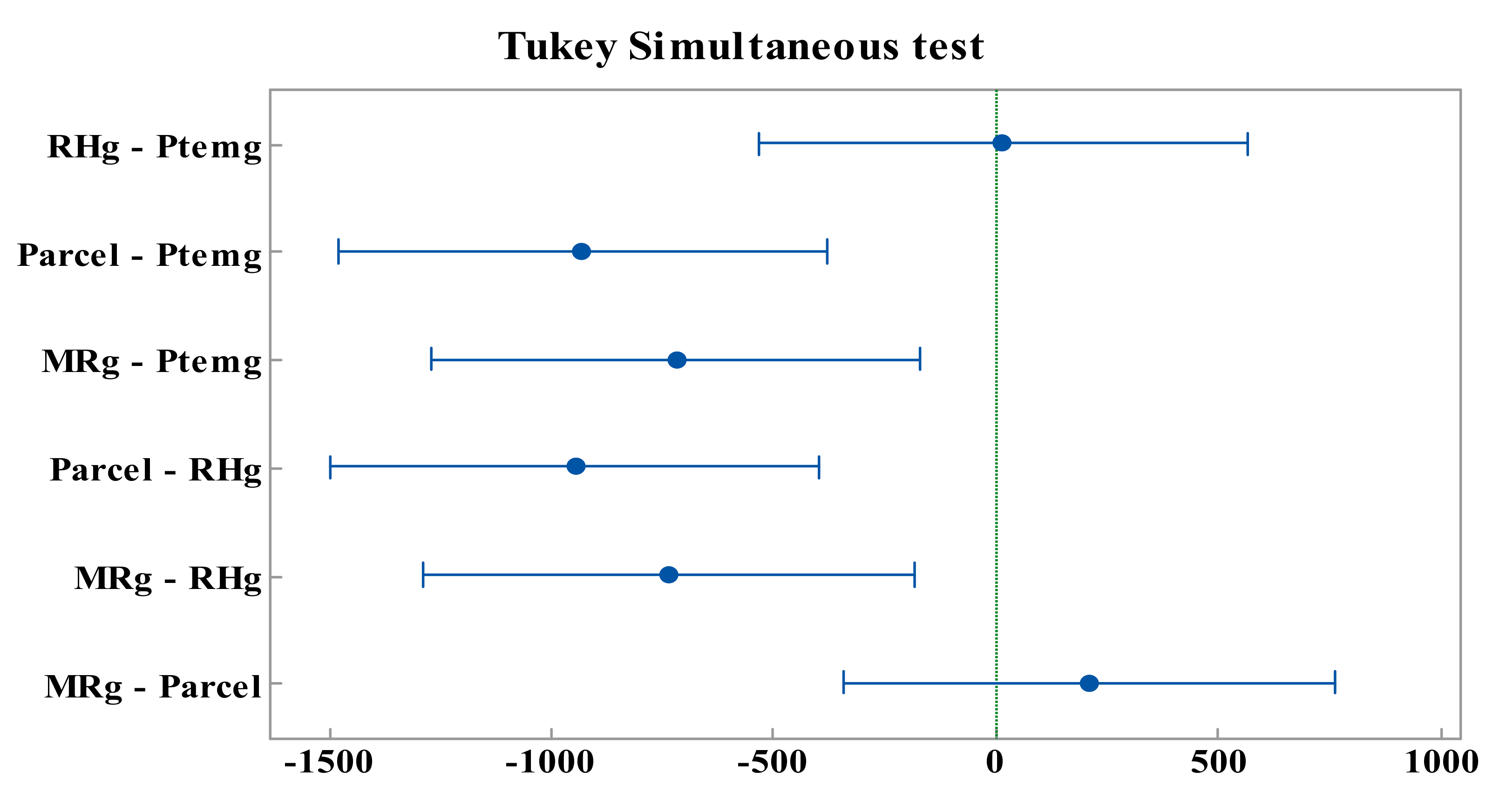
4.1. Comparison of Methods

Descriptive statistics of the ABLH estimated using different methods are presented in Table 1.
The parcel method yielded the lowest mean ABLH. The two radiosonde gradient methods (potential temperature and relative humidity) yielded similar results that are nearly twice as high as that estimated using the parcel method. This discrepancy is consistent with previous results [9]. The mean ABLH estimated using the mixing ratio method is intermediate between the parcel and the radiosonde relative humidity and potential temperature gradient methods. To determine whether the difference between the mean ABLH estimated using different methods are statistically significant, the one-way ANOVA was used. An F-value of 10.52 and p-value less than 0.00001 showed that there is a statistically significant difference between at least two means.
To determine which of the means were significantly different, Tukey’s ad hoc test was used. The result of Tukey’s simultaneous test is presented in Figure A2 in Appendix B. The differences between the mean ABLH estimated using the first two methods (PTemp and RH) and the second two (Parcel and MR) are not statistically significant. However, the other mean comparisons have statistically significant differences.
The Pearson’s correlation coefficients were determined to evaluate the level of linear correlation between ABLH estimated using the different methods. Results of the correlation are presented in Table 2. The correlation coefficients show that the MODIS-derived values are unlikely to be useful to evaluate day-to-day changes in ABLH in this region. The two gradient methods using radiosonde data (relative humidity and potential temperature) show strong positive correlation (R = 0.727) with each other, but the mixing ratio gradient derived from the MODIS data shows extremely weak and even negative correlation with the radiosonde results.

4.2. PM10-ABLH Relationship

Despite the limitation of the MODIS-estimated ABLH, we do observe some success in using it to understand particulate pollution levels. The relationship between the MODIS-estimated ABLH and PM10 mass concentration was evaluated using data from three sites. These three sites represented a range of urbanization: Rubindi is a rural trading center; Mbarara is a small city; and Kyebando is a region of the capital city, Kampala. The hourly mean PM10 and ABLH and the linear regression analysis are presented in Table 3. On average, higher mean ABLH is observed in the afternoon which corresponds to lower values of PM10 mass concentration at all sites. However, the regression analysis for the day-to-day variations varied from no linear correlation to both negative and positive weak correlations that depended on location and time of day.

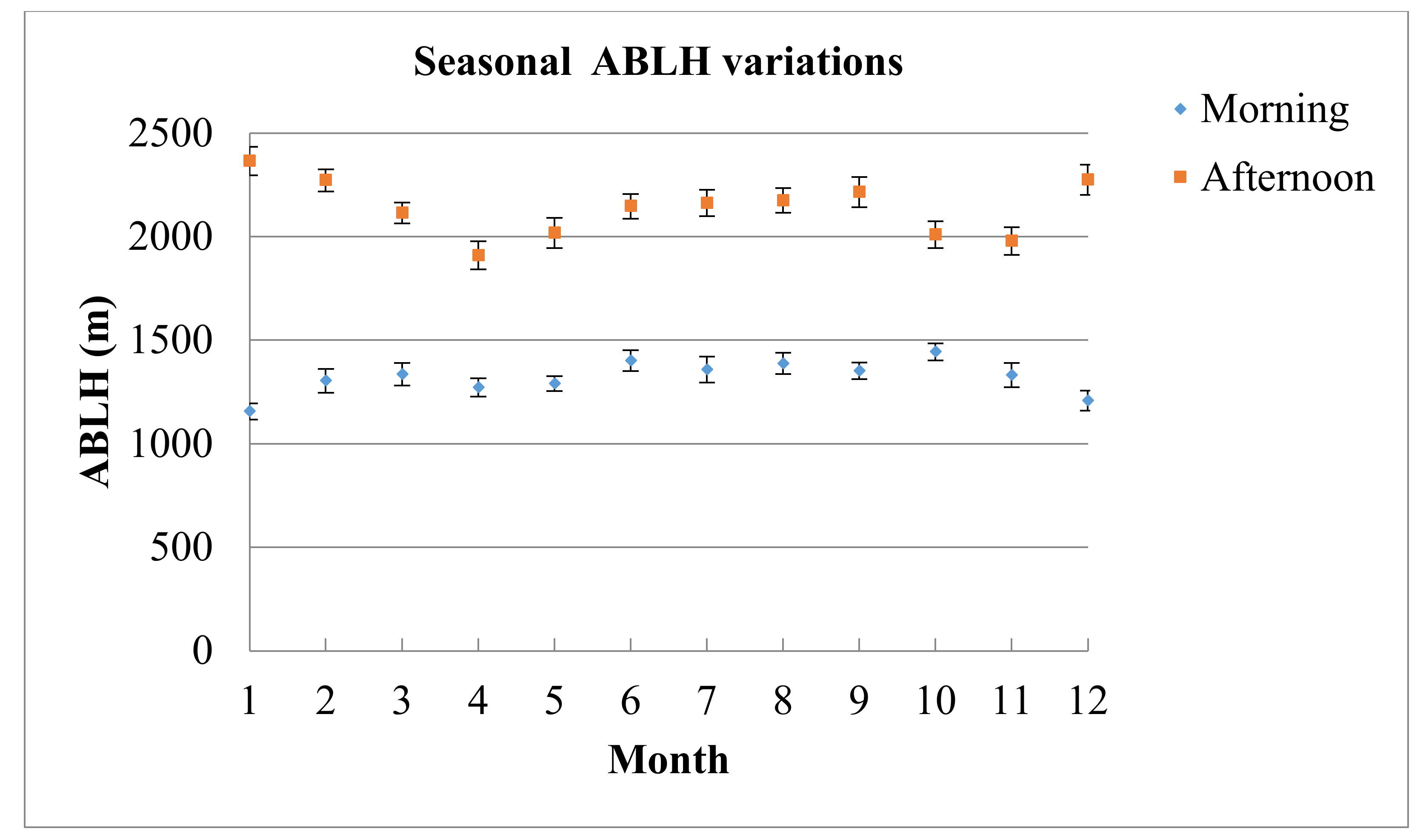
4.3. Temporal Variation of ABLH

The mean ABLH detected using the MODIS data for morning and afternoon observations are presented in Figure 3. These data are averaged over the different regions of Uganda, but similar trends are seen in all the individual regions.
Clear differences are seen between the wet seasons (March–May and Sept–Nov) and the dry seasons (June–Aug and Dec–Feb) in the afternoon ABLH. The afternoon ABLH is higher during the dry seasons than wet seasons. No clear seasonal variations were observed for the morning.

5. Discussion

5.1. Comparison of MODIS and Radiosonde ABLH

There is only a weak and not statistically significant correlation between day-to-day measurements made using MODIS and radiosonde data. Therefore, MODIS cannot normally supplement or replace radiosonde data for determining ABLH.
Differences in the value of ABLH estimated using different methods and profiles have been reported in other studies [9,11,13,15]. For instance, reference [9] showed that ABLH estimated using different methods from the same profiles were significantly different. In their study, the gradient methods estimated ABLH values nearly twice the parcel method [9], so the statistically significant deviation of the parcel method from the radiosonde gradient methods was not surprising. However, a comparison between MODIS and radiosonde ABLH has been previously reported to yield a moderate correlation [18], and that correlation was not observed in the present study.

5.2. MODIS ABLH-PM10 Relationship

The estimated ABLH is related to the daily diurnal variation, with higher PM10 mass concentration in the morning when the ABL is confined closer to the ground and lower PM10 mass concentration in the afternoon when ABL has a greater volume to dilute the particulates. However, the estimated ABLH does not predict day-to-day variation in PM10 mass concentration, with linear correlations ranging from no correlation to weak correlations. A plausible explanation for the short-term day-to-day failure is the differential daily influence of other factors such as relative humidity, wind speed, temperature variation, and source contribution on the PM-ABLH relationship [2]. These factors influence the ABLH and PM mass concentrations differently resulting in a weak PM-ABLH relationship. When averaged over a longer period, these influences seem to cancel out.
Other studies [1,3,7,8,10] that used different sources of profile data to evaluate the PM-ABLH relationship reported similar results. For instance, reference [2] used LIDAR observations to evaluate the ABLH-PM relationship over China. They reported that the PM-ABLH correlations are roughly negative for most cases, with magnitude, significance, and even sign varying considerably with location, season, and meteorological conditions. In some cases, weak or even an uncorrelated PM-ABLH relationship was reported. Reference [3] evaluated the relations between PM2.5 and ABLH over China during winter using Mie LIDAR observations. They reported a significant negative correlation.

5.3. Temporal Variations

As shown in Figure 3, the mean MODIS-derived ABLH for each month was higher in the afternoon than morning at all locations. Morning and afternoon differences are due to the effect of cumulative surface heating. Surface heating starts at sunrise, escalating as the day progresses [5,8]. In the process, air above the surface cumulatively retains more and more heat leading to a gradual increase in convection within the lower layers of the atmosphere. The result is a gradual increase in turbulence and a cumulative volume increase in the ABL. It has been shown that ABLH starts to significantly increase at about 09:00 and peaks at about 15:00 LST [8,14,27].
The mean dry season ABLH is higher than the wet season ABLH. Seasonal differences in the ABLH are a consequence of differences in the rate of both surface heating and cooling during the two seasons. Greater surface heating due to the absence of both cloud cover and rain fall is usually experienced during the dry season, while surface cooling is dominant during the wet seasons due to the presence of both cloud cover and rainfall [28]. Both temperature and cloud cover have been shown to influence ABLH in other parts of the world [7,8]. Seasonal differences in the ABLH have been reported in other studies. For instance, reference [7] observed that ABLH values are in the order spring > summer > fall > winter in most parts of China. They also showed that surface temperature and wind speed negatively influence ABLH. Moreover, reference [5] showed that there are significant seasonal and diurnal variations in the ABLH worldwide, while reference [29] showed that there are significant seasonal differences in the estimated ABLH.

6. Conclusions

In this study, the MODIS atmospheric profile data were used to estimate ABLH in Uganda. The correlation between the radiosonde and MODIS ABLH is weak and not statistically significant. Therefore, the ABLH estimated using MODIS atmospheric profiles is not a good alternative to the radiosonde profile for estimating the ABLH in Uganda, at least when using automated calculations to determine the ABLH that do not account for cloud cover and local conditions. However, the ABLH-PM10 relationship is similar to that observed in other studies in which other sources of atmospheric profile data were used, and on average the MODIS-derived ABLH is higher during dry than rainy months and in the afternoon than morning, as expected.

Author Contributions

Conceptualization, S.O. and G.A.; methodology, S.O., G.A., and B.P.; software, G.A. and B.P.; validation, B.P. and S.K.A.; formal analysis, S.O.; investigation, S.O.; writing—original draft preparation, S.O.; writing—review and editing, G.A., B.P., and S.K.A. The manuscript was critically reviewed by all authors. All authors have participated sufficiently in the work to take public responsibility for appropriate portions of the content and agreed to be accountable for all aspects of the work in ensuring that questions related to the accuracy or integrity of any part of the work are appropriately investigated and resolved. All authors have read and agreed to the published version of the manuscript.

Funding

Support for this research was provided by the US Fulbright Scholar Program, the Research Council of Colgate University, and Mbarara University of Science and Technology.

Conflicts of Interest

The authors declare no conflict of interest and the funders had no role in the design of the study; in the collection, analysis, or interpretation of data; in the writing of the manuscript, or in the decision to publish the results.

Appendix A

Table A1. Points of reference for the retrieval of MODIS atmospheric profiles. Letters are adopted from Figure 1.
SiteReferencelatitudeLongitudeAltitude
AruaJ3.02030.8751310
GuluI2.77832.2941100
EntebbeA20.05032.4501155
KaseseM0.17530.0861000
KibogaL0.91531.7651180
KitgumH3.29832.881760
KotidoG3.00634.1141260
MasakaA1−0.33431.7321288
NakasongolaB1.31432.4591160
NebbiK2.47931.089981
NtungamoC−0.87230.2661400
SironkoF1.23134.2481178
SorotiE1.73833.6221080
TororoD0.68134.1661278
Figure A1. Spatial variations in the availability of estimated ABLH. The reference line represents a fraction below which observations would be deemed too few for statistical analysis.
Atmosphere 11 00908 g0a1

Appendix B

Figure A2. Tukey’s simultaneous test for difference of the mean ABLH estimated using different methods. Results are reported at 95% confidence level. For pairs where the interval does not possess a zero, the difference is statistically significant.
Atmosphere 11 00908 g0a2

References

  1. Seo, S.; Kim, J.; Lee, H.; Jeong, U.; Kim, W.; Holben, B.N.; Kim, S.-W.; Song, C.H.; Lim, J.H. Estimation of PM 10 concentrations over Seoul using multiple empirical models with AERONET and MODIS data collected during the DRAGON-Asia campaign. Atmos. Chem. Phys. 2015, 15, 319–334. [Google Scholar] [CrossRef] [Green Version]
  2. Su, T.; Li, Z.; Kahn, R. Relationships between the planetary boundary layer height and surface pollutants derived from lidar observations over China: Regional pattern and influencing factors. Atmos. Chem. Phys. 2018, 18, 15921–15935. [Google Scholar] [CrossRef] [Green Version]
  3. Xiang, Y.; Zhang, T.; Liu, J.; Lv, L.; Dong, Y.; Chen, Z. Atmosphere boundary layer height and its effect on air pollutants in Beijing during winter heavy pollution. Atmos. Res. 2019, 215, 305–316. [Google Scholar] [CrossRef]
  4. Yap, X.Q.; Hashim, M. A robust calibration approach for PM10 prediction from MODIS aerosol optical depth. Atmos. Chem. Phys. 2013, 13, 3517–3526. [Google Scholar] [CrossRef] [Green Version]
  5. Davy, R. The climatology of the atmospheric boundary layer in contemporary global climate models. J. Clim. 2018, 31, 9151–9173. [Google Scholar] [CrossRef]
  6. Davy, R.; Esau, I. Differences in the efficacy of climate forcings explained by variations in atmospheric boundary layer depth. Nat. Commun. 2016, 7, 1–8. [Google Scholar] [CrossRef] [PubMed]
  7. Guo, J.; Miao, Y.; Zhang, Y.; Liu, H.; Li, Z.; Zhang, W.; He, J.; Lou, M.; Yan, Y.; Bian, L. The climatology of planetary boundary layer height in China derived from radiosonde and reanalysis data. Atmos. Chem. Phys. 2016, 16, 13309. [Google Scholar] [CrossRef] [Green Version]
  8. Liu, S.; Liang, X.-Z. Observed diurnal cycle climatology of planetary boundary layer height. J. Clim. 2010, 23, 5790–5809. [Google Scholar] [CrossRef]
  9. Seidel, D.J.; Ao, C.O.; Li, K. Estimating climatological planetary boundary layer heights from radiosonde observations: Comparison of methods and uncertainty analysis. J. Geophys. Res. Atmos. 2010, 115, D16113. [Google Scholar] [CrossRef] [Green Version]
  10. Du, C.; Liu, S.; Yu, X.; Li, X.; Chen, C.; Peng, Y.; Dong, Y.; Dong, Z.; Wang, F. Urban boundary layer height characteristics and relationship with particulate matter mass concentrations in Xi’an, central China. Aerosol Air Qual. Res. 2013, 13, 1598–1607. [Google Scholar] [CrossRef]
  11. Basha, G.; Ratnam, M.V. Identification of atmospheric boundary layer height over a tropical station using high-resolution radiosonde refractivity profiles: Comparison with GPS radio occultation measurements. J. Geophys. Res. Atmos. 2009, 114, D16101. [Google Scholar] [CrossRef]
  12. Dang, R.; Yang, Y.; Hu, X.-M.; Wang, Z.; Zhang, S. A review of techniques for diagnosing the atmospheric boundary layer height (ABLH) using aerosol lidar data. Remote Sens. 2019, 11, 1590. [Google Scholar] [CrossRef] [Green Version]
  13. Kotthaus, S.; Grimmond, C.S.B. Atmospheric boundary-layer characteristics from ceilometer measurements. Part 1: A new method to track mixed layer height and classify clouds. Q. J. R. Meteorol. Soc. 2018, 144, 1525–1538. [Google Scholar] [CrossRef] [Green Version]
  14. Wang, X.; Wang, K. Homogenized variability of radiosonde-derived atmospheric boundary layer height over the global land surface from 1973 to 2014. J. Clim. 2016, 29, 6893–6908. [Google Scholar] [CrossRef]
  15. Hennemuth, B.; Lammert, A. Determination of the atmospheric boundary layer height from radiosonde and lidar backscatter. Bound. Layer Meteorol. 2006, 120, 181–200. [Google Scholar] [CrossRef]
  16. McGrath-Spangler, E.L.; Molod, A. Comparison of GEOS-5 AGCM planetary boundary layer depths computed with various definitions. Atmos. Chem. Phys. 2014, 14, 6717–6727. [Google Scholar] [CrossRef] [Green Version]
  17. Durre, I.; Yin, X.; Vose, R.S.; Applequist, S.; Arnfield, J. Enhancing the data coverage in the Integrated Global Radiosonde Archive. J. Atmos. Ocean. Technol. 2018, 35, 1753–1770. [Google Scholar] [CrossRef]
  18. Feng, X.; Wu, B.; Yan, N. A method for deriving the boundary layer mixing height from modis atmospheric profile data. Atmosphere 2015, 6, 1346–1361. [Google Scholar] [CrossRef] [Green Version]
  19. Borbas, E.; Menzel, P. MODIS Atmosphere L2 Atmosphere Profile Product. In NASA MODIS Adaptive Processing System; Goddard Space Flight Center: Greenbelt, MD, USA, 2017. [Google Scholar]
  20. Remer, L.A.; Mattoo, S.; Levy, R.C.; Munchak, L.A. MODIS 3 km aerosol product: Algorithm and global perspective. Atmos. Meas. Tech. 2013, 6, 1829–1844. [Google Scholar] [CrossRef] [Green Version]
  21. Onyango, S.; Parks, B.; Anguma, S.; Meng, Q. Spatio-Temporal Variation in the Concentration of Inhalable Particulate Matter (PM10) in Uganda. Int. J. Environ. Res. Public Health 2019, 16, 1752. [Google Scholar] [CrossRef] [Green Version]
  22. Levy, R.C.; Mattoo, S.; Munchak, L.A.; Remer, L.A.; Sayer, A.M.; Patadia, F.; Hsu, N.C. The Collection 6 MODIS aerosol products over land and ocean. Atmos. Meas. Tech. 2013, 6, 2989. [Google Scholar] [CrossRef] [Green Version]
  23. Belle, J.; Liu, Y. Evaluation of aqua modis collection 6 aod parameters for air quality research over the continental united states. Remote Sens. 2016, 8, 815. [Google Scholar] [CrossRef] [Green Version]
  24. Dudeja, J.P. Micro-Pulse Lidar for the Determination of Atmospheric Boundary Layer Height. Int. J. Res. Anal. Rev. 2019, 6, 810. [Google Scholar]
  25. Basalirwa, C.P.K. Delineation of Uganda into climatological rainfall zones using the method of principal component analysis. Int. J. Climatol. 1995, 15, 1161–1177. [Google Scholar] [CrossRef]
  26. Rugumayo, A.I.; Kiiza, N.; Shima, J. Rainfall reliability for crop production a case study in Uganda. In Proceedings of the Diffuse Pollution Conference, Dublin, Ireland, 17–21 August 2003; Volume 3, pp. 143–148. [Google Scholar]
  27. Mehta, S.K.; Ratnam, M.V.; Sunilkumar, S.V.; Rao, D.N.; Krishna Murthy, B.V. Diurnal variability of the atmospheric boundary layer height over a tropical station in the Indian monsoon region. Atmos. Chem. Phys. 2017, 17, 531–549. [Google Scholar] [CrossRef]
  28. Nsubuga, F.W.; Rautenbach, H. Climate change and variability: A review of what is known and ought to be known for Uganda. Int. J. Clim. Chang. Strateg. Manag. 2018, 10, 752–771. [Google Scholar] [CrossRef] [Green Version]
  29. Zhang, Y.; Gao, Z.; Li, D.; Li, Y.; Zhang, N.; Zhao, X.; Chen, J. On the computation of planetary boundary-layer height using the bulk Richardson number method. Geosci. Model Dev. 2014, 7, 2599–2611. [Google Scholar] [CrossRef] [Green Version]
Figure 1. Map of Uganda showing the climatic zones of Uganda that were used in this project (adapted from Reference [26]). The locations listed in Table A1 are shown as blue dots on the map, and the location that was also the site of radiosonde launches (Entebbe) is shown as a large green dot.
Atmosphere 11 00908 g001
Figure 2. Relative humidity (from radiosondes), potential temperature (from radiosondes), and mixing ratio profiles (from MODIS) for twelve dates at Entebbe airport. The horizontal blue lines show the ABLH determined from gradients of these values.
Atmosphere 11 00908 g002
Figure 3. Mean ABLH in the morning and afternoon for months 1–12 (Jan–Dec). The mean was computed using data from the fourteen locations described in Table A1. The error bars show the standard error of the mean.
Atmosphere 11 00908 g003
Table 1. The atmospheric boundary layer height (ABLH) values estimated using radiosonde data (PTemp, RH, and Parcel) and moderate resolution spectroradiometer (MODIS) data (MR). PTemp, RH, and MR are the potential temperature gradient, relative humidity gradient, and mixing ratio gradient methods, respectively. N is the number of samples; SEM is the standard error of the mean; SD is the standard deviation; Q1 is the first quartile value; and Q3 is the third quartile value.
MethodNMean ± SEMSDMinimumQ1MedianQ3Maximum
PTemp532049 ± 1841338227722190833203986
RH532066 ± 199144930653226235503986
Parcel531121 ± 68497236818107314212584
MR531330 ± 112815350367118921483482
Table 2. Correlation of ABLH estimated using different methods. RH is the relative humidity gradient (radiosonde); PTemp is the potential temperature gradient (radiosonde); and MR is the mixing ratio gradient method (MODIS). Within each cell, the upper number is the correlation coefficient (R), and the lower number is the p-value for the significance of the correlation. p-values less than 0.05 are considered significant.
MethodPTempRHParcel
RH0.727
0.000
Parcel0.2270.164
0.1030.241
MR0.020−0.1280.030
0.8890.3620.833
Table 3. Effect of MODIS estimated ABLH on PM10 mass concentration at selected sites. R is the correlation coefficient and p is the p-value of the correlation, with values under 0.05 considered to be significant.
Site PM
(μg m−3)
ABLH
(m)
Rp
MbararaMorning72.8 ± 15.01439 ± 154−0.0600.812
Afternoon62.7 ± 14.12344 ± 1430.3730.209
RubindiMorning68.9 ± 9.071583 ± 132−0.2540.325
Afternoon65.7 ± 16.22449 ± 2230.4650.029
KyebandoMorning85.7 ± 10.7900 ± 1390.2700.372
Afternoon77.1 ± 15.72400 ± 1050.0020.996

