Insights for Air Quality Management from Modeling and Record Studies in Cuenca, Ecuador


1
Instituto de Simulación Computacional, Colegio de Ciencias e Ingenierías, Universidad San Francisco de Quito USFQ, Quito 170901, Ecuador
2
Red de Monitoreo de Calidad del Aire de Cuenca-EMOV, Cuenca 010206, Ecuador
*
Author to whom correspondence should be addressed.
Atmosphere 2020, 11(9), 998; https://0-doi-org.brum.beds.ac.uk/10.3390/atmos11090998
Submission received: 24 August 2020
/
Revised: 10 September 2020
/
Accepted: 12 September 2020
/
Published: 18 September 2020
(This article belongs to the Special Issue Coronavirus Pandemic Shutdown Effects on Urban Air Quality)
Abstract
:On-road traffic is the primary source of air pollutants in Cuenca (2500 m. a.s.l.), an Andean city in Ecuador. Most of the buses in the country run on diesel, emitting high amounts of NOx (NO + NO2) and PM2.5, among other air pollutants. Currently, an electric tram system is beginning to operate in this city, accompanied by new routes for urban buses, changing the spatial distribution of the city’s emissions, and alleviating the impact in the historic center. The Ecuadorian energy efficiency law requires that all vehicles incorporated into the public transportation system must be electric by 2025. As an early and preliminary assessment of the impact of this shift, we simulated the air quality during two scenarios: (1) A reference scenario corresponding to buses running on diesel (DB) and (2) the future scenario with electric buses (EB). We used the Eulerian Weather Research and Forecasting with Chemistry (WRF-Chem) model for simulating the air quality during September, based on the last available emission inventory (year 2014). The difference in the results of the two scenarios (DB-EB) showed decreases in the daily maximum hourly NO2 (between 0.8 to 16.4 µg m−3, median 7.1 µg m−3), and in the 24-h mean PM2.5 (0.2 to 1.8 µg m−3, median 0.9 µg m−3) concentrations. However, the daily maximum 8-h mean ozone (O3) increased (1.1 to 8.0 µg m−3, median 3.5 µg m−3). Apart from the primary air quality benefits acquired due to decreases in NO2 and PM2.5 levels, and owing to the volatile organic compounds (VOC)-limited regime for O3 production in this city, modeling suggests that VOC controls should accompany future NOx reduction for avoiding increases in O3. Modeled tendencies of these pollutants when moving from the DB to EB scenario were consistent with the tendencies observed during the COVID-19 lockdown in this city, which is a unique reference for appreciating the potentiality and identifying insights for air quality improvements. This consistency supports the approach and results of this contribution, which provides early insights into the effects on air quality due to the recent operability of the electric tram and the future shift from diesel to electric buses in Cuenca.
1. Introduction
On-road traffic is one of the most important sources of air pollutants in cities located in Ecuador [1,2]. Emissions from this source are exacerbated for cities located in the Andean region of the country, owing to their altitude, where the content of atmospheric oxygen is lower compared to at sea level. Therefore, combustion processes emit more primary pollutants in these cities [3].
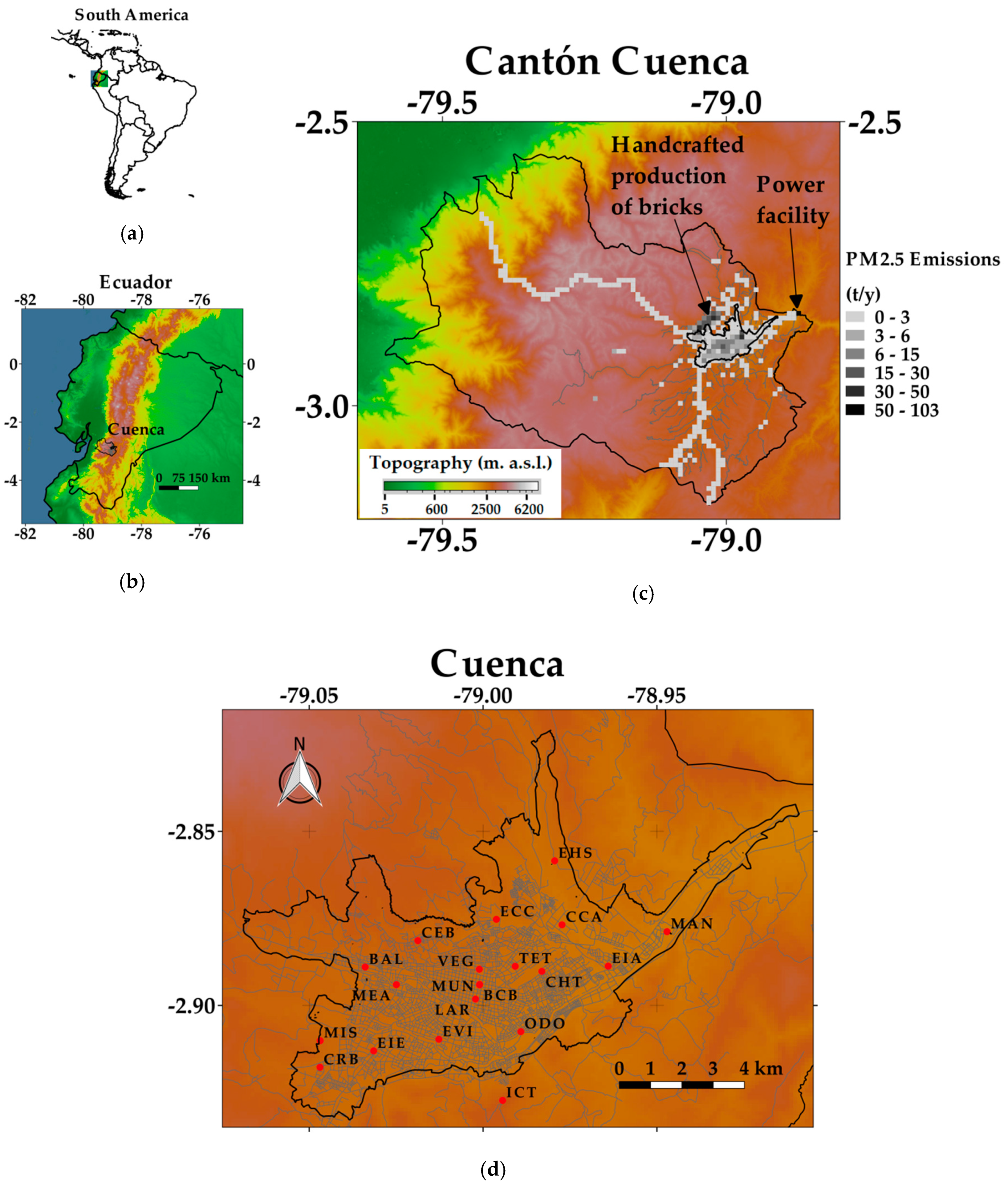
In Cuenca (Lon. −79.0°, Lat. −2.9°, 2500 m. a.s.l.), which is a city located in the Southern Andean region of the country (Figure 1), during 2014, on-road traffic, among other pollutants, emitted 5981.0 and 384.0 t y−1 of NOx (NO + NO2) and PM2.5, respectively, representing 71.2% and 42.2% of the total emissions of each pollutant [4].
NOx (NO + NO2) is mainly produced by the combination of atmospheric N2 and O2, when, under high temperatures and pressures, air is mixed with fuel in engines. Diesel engines work at pressures 1.5 times higher than those of gasoline engines of a comparable power [5], producing high quantities of NOx. Additionally, diesel vehicles emit 10 to 100 times more particulate mass than gasoline vehicles [6] and are major sources of nanoparticles [7].
Ozone (O3) is a secondary air pollutant produced from photochemical interactions between NOx and volatile organic compounds (VOC), through complex reactions under the influence of solar radiation [8]. Sources of VOC are diverse, including gasoline cars, service stations, the use of solvents, and vegetation.
NO2 can increase the airway reactivity to cold air in asthmatics and the susceptibility to bacterial and viral infections of the lung [9]. O3 is a strong oxidant and reactive pollutant, which increases the airway responsiveness, airway inflammation, respiratory infections, tissue permeability, exacerbation of asthma, and pulmonary function impairment [9,10].
PM2.5 exhibits effects after both short-term and long-term exposure. Current World Health Organization (WHO) guidelines cannot guarantee complete protection against PM2.5 effects [11], thus requiring the lowest possible concentrations to be achieved. Short-term exposition includes cardiovascular and respiratory effects. The International Agency for Research on Cancer (IARC) has classified outdoor air pollution and particulate matter from outdoor air pollution as carcinogenic to humans [12,13].
Although it was previously considered that air pollution mainly affects the lungs and cardiovascular system, recent literature has reported that it also threatens brain health, promoting Alzheimer’s disease and affecting cognitive, behavioral, and academic performances [14,15,16]. In terms of brain effects, particulate matter is the component of air pollution that appears to be the most concerning [17].
1.1. Emission Inventory from Cuenca
The municipality of Cuenca currently has about 640,000 inhabitants. It has a complex topography, with altitudes ranging from 1000 to 4000 m. a.s.l. (Figure 1). Table 1 presents a summary of the emission inventory from 2014 [4]. The total emission of NOx was 8402 t y−1, with on-road traffic (71.2%) and a power facility (18.5%) located in the northeast of the city being the most significant source. The total emission of PM2.5 was 907 t y−1, with on-road traffic (42.4%), the handcrafted production of bricks (38.5%), and the power facility (11.3%) being the most significant sources. The handcrafted production of bricks corresponds to about 600 artisanal producers, mainly located in the northwest, outside of the urban area. The power facility is also situated outside of the urban area of Cuenca.
Buses emitted 1861.2 and 87.2 t y−1 of NOx and PM2.5, respectively, representing 31.1% and 22.7% of the total on-road traffic emissions of each pollutant (Table 2). Even heavy diesel vehicles emitted higher quantities of NOx and PM2.5, compared with buses, producing 36.9% and 63.4%, respectively, of the total on-road traffic emissions of each. Gasoline vehicles emitted 30.3% and 7.0% of the NOx and PM2.5 from on-road traffic.
The total emission of non-methane volatile organic compounds (NMVOC) was 15,310 t y−1, with on-road traffic (39.6%), the use of solvents (29.7%), and vegetation (19.5%) being the most important sources (Table 1). Gasoline cars emitted 72.8% of the NMVOC from on-road traffic (Table 2), representing a priority source that needs to be controlled. NMVOC from on-road traffic includes exhaust and evaporative (diurnal emissions, running losses, and hot-soak emissions) emissions.
The number of buses considered in the emission inventory from 2014 was 2304 [4]. This quantity includes urban buses, whose total is currently 475 units. According to the Ecuadorian regulation, the public transport service comprises the following areas of operation: Urban, intraregional, interprovincial, national, and international.
The quality of hourly emission maps derived from the emission inventory from 2014 [4], which is the most recent, was verified when these emissions were incorporated into a 3D-Eulerian model for studying the influence of six planetary boundary layer schemes for modeling the air quality in Cuenca [18]. Modeling is also a powerful approach for foreseeing the effects on air quality, due to changes in the emission inventories [19], which can help define policies, programs, and projects for air quality management.
1.2. The Air Quality from Cuenca
The air quality stations are mainly located in the urban area. There is one automatic station located in the historic center (MUN station, Figure 1), which, since 2012, has monitored the short-term air quality (CO, NO2, PM2.5, and O3) and meteorology [20]. Additionally, there are about 20 passive stations for measuring monthly-mean air quality concentrations (NO2 and O3). Measurement of the air quality is based on the methods established in the Ecuadorian air quality regulation under the responsibility of the Municipality of Cuenca, which, for this purpose, is the entity accredited by the National Environmental Authority. The air quality network’s current equipment is described in the report on the air quality from 2019 [20], which corresponds to the directives established by the USA Environmental Protection Agency and European. As part of its operation, corresponding quality assurance and quality control activities are permanently performed.
From 2012 to 2019, all daily records of NO2 (maximum 1-h mean) were lower than the WHO guideline (200 µg m−3). From 2008 to 2019, the annual mean NO2 concentrations (passive stations) varied between 5.5 and 47.2 µg m−3 [20,21,22,23,24,25,26]. Annual mean NO2 concentrations higher than the WHO guideline (40 µg m−3) [11] were measured at Bomberos (BCB) and Vega Muñoz (VEG), which are microscale stations located at a street canyon supporting the high level of traffic of gasoline and diesel (buses) vehicles.
From 2012 to 2019, during fourteen days, the PM2.5 concentrations (24-h mean) were higher than the WHO guideline (25 µg m−3). The annual mean PM2.5 concentrations varied between 6.1 and 10.8 µg m−3. During four years in this period, this mean was higher than the WHO guideline (10 µg m−3, [11]).
From 2012 to 2019, the maximum 8-h mean O3 concentrations were higher than the WHO guideline (100 µg m−3) during specific days from March 2013 (8), April 2013 (5), September 2015 (2), and September 2017 (3).
Studying the growing historical dataset or air quality records promotes the understanding of the complex behavior of air pollutants in Cuenca. Based on the records from 2013 to 2015, the weekend effect (WE), which is a phenomenon characterized by increased concentrations of O3 during weekends, although the emissions of NOx and VOC are typically lower in comparison to weekdays, was identified in the urban area of Cuenca [27], suggesting the presence of a VOC-limited regime for O3 production. This finding provided the first insights into the influence of decreased on-road traffic emissions during weekends.
1.3. Actions for Controlling Air Pollutant Emissions
One of the most relevant controls of air pollutant emissions in Cuenca is the technical vehicular revision (RTV, due to its acronym in Spanish). According to the RTV regulation, it is mandatory that vehicles running in Cuenca must demonstrate each year that their exhaust emissions are lower than the levels established in the national regulation as a requirement to allow their use. Currently, through the RTV, CO and HC emissions from gasoline cars and the opacity of diesel vehicle emissions are measured. Today, NOx emissions from on-road traffic are not controlled.
Another component currently affecting air pollutant emissions is the operation of an electric tram, conceived as the new core of the public transportation system of Cuenca that aims to solve the problems associated with on-road traffic. The building of this facility began at the end of 2013. However, different problems and conflicts have appeared related to restricted mobility and effects on local commercial activities [28]. After several years of delay, the electric tram began to work during the time of writing this manuscript. The electric tram alleviates the air pollutant emissions along its route, which includes the historic center. However, the displaced buses will move their emissions to new routes.
In the future, under the framework of the Ecuadorian energy efficiency law [29], all vehicles incorporated into the public transportation system must be electric by 2025. The shift from diesel to electric buses will eliminate or reduce the exhaust emissions from diesel buses, decreasing, as a consequence, the NOx and PM2.5 emissions.
1.4. The Forced Lockdown Owing to COVID-19
To reduce the spread of COVID-19, several measures, such as lockdowns, quarantine, stay at home, and transportation restrictions were applied world-wide. The corresponding effects on air quality have begun to be reported from different regions. Nakada and Urban (2020) [30] reported drastic reductions in NO, NO2, and CO in Sao Paulo (Brazil), although an increase in O3 concentrations. Jia et al. (2020) [31] reported an insignificant impact on reducing air pollution in Memphis (U.S.A.). Sicard et al. (2020) [32] reported increased O3 concentrations in four European cities (Nice, Rome, Valencia, and Turin) and Wuhan (China). Otmani et al. (2020) [33] reported reductions in PM10, SO2, and NO2 in Salé (Morocco).
In Ecuador, based on the infected people and the pandemic declaration by WHO, the government declared (decree 1017) the exception status on 16 March 2020 [34]. One of the measures of this status was a restriction on mobility. During the following days, on-road traffic and other activities notably reduced, therefore decreasing the emission of air pollutants.
Although the exception status was officially maintained in Cuenca until 24 May 2020, some activities restarted on 17 May 2020 [35]. On 25 May 2020, the status was relaxed, alleviating the restriction of on-road traffic and other activities, and allowed buses employed for regional transportation to reactivate their service. Since 01 June 2020, urban buses in Cuenca have returned to service.
The air quality records from the exception status provide a unique opportunity to learn and appreciate the potentiality for air quality improvement as a consequence of the decrease in activities, such as on-road traffic.
This contribution explores the following issues of the air quality in Cuenca:
- Verification of the presence of the WE in Cuenca after 2015;
- The effects on air quality due to the future shift from diesel to electric buses;
- The air quality during the COVID-19 lockdown, and its comparison to previous weeks and years;
- A holistic analysis of these interrelated components to identify insights for air quality management.
2. Method
2.1. WE in Cuenca
To complete the analysis of 2013 to 2015, and based on the same approach presented in Parra (2017) [27], we obtained mean-daily profiles for CO, NO2, PM2.5, and O3 for each year of the period 2016 to 2019, and considering weekdays, Saturdays, and Sundays. We obtained the maximum 8-h mean O3 concentrations to quantify the variation (percentage) of this pollutant from Saturdays and Sundays, compared to weekdays. These O3 concentrations were obtained from the hourly values obtained between 9:00 and 16:00, considering that, during this period, typically, the O3 concentrations are higher. This approach was used in a study of the WE in Santiago (Chile) [36] and Quito (Ecuador) [37].
2.2. Shift from Diesel to Electric Buses
As an early and preliminary assessment of the impact owing to the shift from diesel to electric buses, established in the Ecuadorian efficiency law, we simulated the air quality in Cuenca under two scenarios: (1) A reference scenario corresponding to buses running on diesel (DB) and (2) the future scenario with electric buses (EB). We used the Eulerian Weather Research and Forecasting with Chemistry (WRF-Chem V3.2) model [38] for simulating the air quality during September of 2014, based on the most recent emission inventory of Cuenca [4]. WRF-Chem is a state-of-the-art chemical transport model that requires, as the input, hourly maps of speciated emissions. Hourly maps were built using factors for activity data, considering the differences between weekdays and weekends and the influence of meteorology on vegetation emissions. September was selected because its on-road traffic and other activity levels are representative for the other months. Additionally, during specific days of September 2015 (2) and September 2017 (3), O3 concentrations were higher than the WHO guideline (100 µg m−3, maximum 8-h mean), partly due to the high levels of near zenith solar radiation reaching the region of Ecuador during this month.
For the DB scenario, all of the emissions sources of Table 1 were included when building the hourly emissions maps. For the EB scenario, as a first assumption, all of the combustion emissions (NOx, CO, NMVOC, SO2, PM10 exhaust, and PM2.5 exhaust) from buses (Table 2) were eliminated.
Initial and boundary conditions were generated using the final National Centers for Environmental Prediction (NCEP FNL) Operational Global Analysis data [39]. Meteorological simulations were carried out using a master domain of 70 × 70 cells (27 × 27 km each) and three nested sub-domains. The third sub-domain (100 × 82 cells of 1 km each, and 35 vertical levels) covers the region of the Cantón Cuenca (Figure 1). For the third sub-domain, the option of WRF-Chem for the chemical transportation of pollutants was activated, selecting the carbon bond mechanism–Z (CBMZ) [40] for gaseous pollutants and the model for simulating aerosols interactions and chemistry (MOSAIC) for aerosols [41]. One crucial feature of WRF-Chem is the possibility to apply online approach modeling, allowing simultaneous treatment with feedback between meteorological and air quality variables. For this study, the option for direct effects between aerosols and meteorology was activated, using four aerosol bins. Working with direct effects improved the performance when modeling the air quality in Cuenca, compared to modeling without feedback [18].
2.3. Air Quality during the COVID-19 Lockdown
We compared the short-term air quality (maximum 8-h mean CO, maximum 1-h mean NO2, 24-h mean PM2.5, and maximum 8-h mean O3) records obtained from the MUN station during 17 March 2020 to 16 May 2020 (61 days), with records from the following periods:
- Weeks before the exception status (01 January 2020 to 16 March 2020), and;
- From 17 March to 16 May, of previous years, from 2015 to 2019. Although there is information available from 2012, we selected 2015 onwards, because records after this year covered at least 70% of days. We selected this percentage to assure the representativeness of records.
The short-term air quality concentrations used for comparison are congruent with the WHO guidelines [9,11] and the Ecuadorian air quality regulation. The maximum 1-h mean corresponds to the maximum hourly mean concentration per day. The maximum 8-h mean corresponds to the maximum mean concentration for eight consecutive hours per day. We conducted Wilcoxon tests to establish if the distributions were statistically equal or different.
3. Results and Discussion
3.1. WE in Cuenca
In agreement with the results from 2013 to 2015 [27], from 2016 to 2019, the mean-daily profiles of CO, NO2, and PM2.5 showed lower concentrations on Saturdays and Sundays, compared to weekdays. However, O3 profiles were higher. Figure 2 depicts the profiles from 2018. The profiles of other years presented similar configurations.
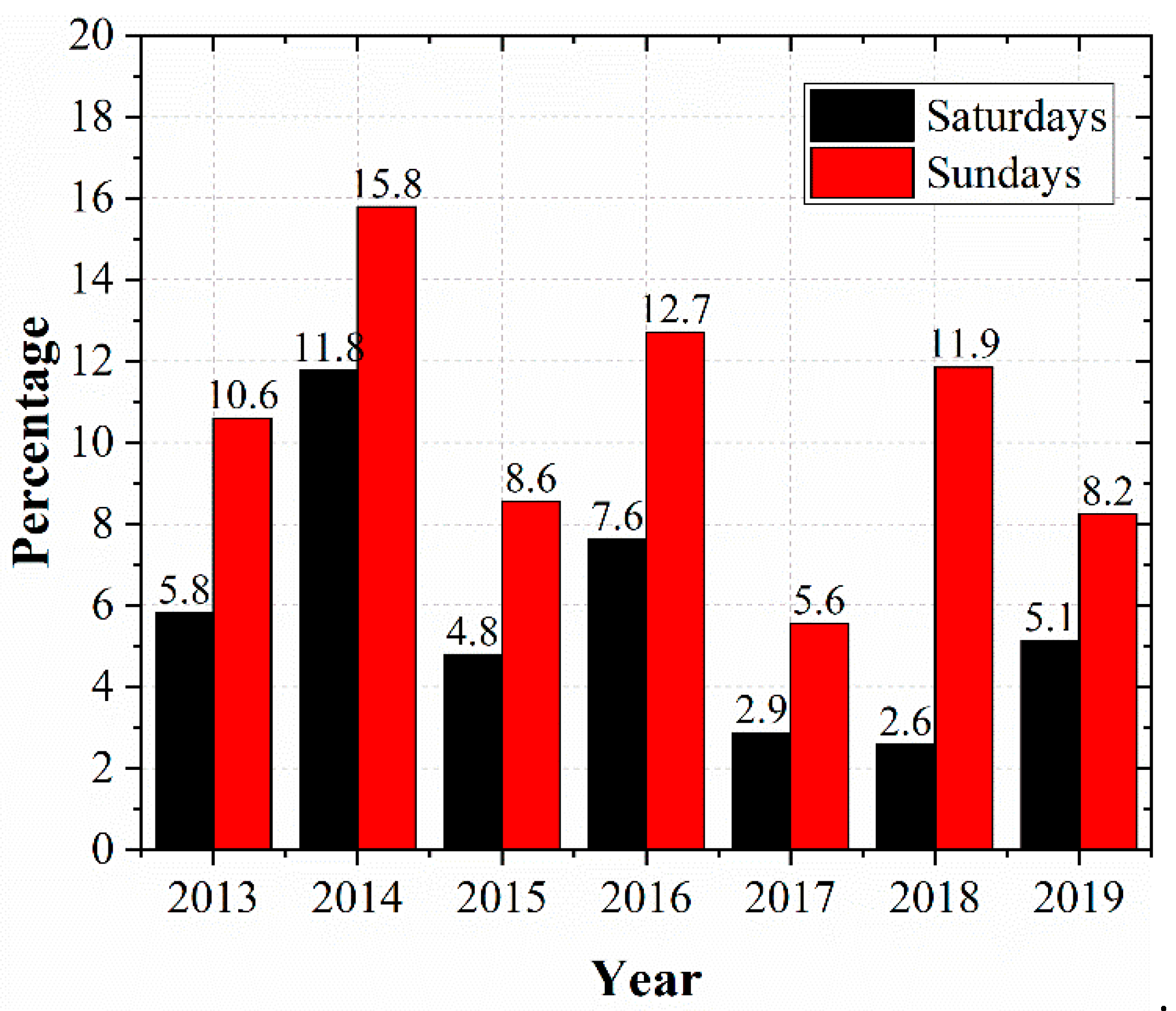
From 2013 to 2019, the increase in the maximum 8-h mean O3 concentrations of Saturdays and Sundays compared to weekdays varied between 2.6% and 11.8% and 5.6% and 15.8%, respectively (Figure 3). Although we limited our analysis to the yearly period, our results confirm the presence of the WE in the urban area of Cuenca, where on-road traffic is the most relevant air pollutant source. More insights can be drawn in the future, through an analysis of the historical records per season or month.
Diesel vehicles, representing 10.8% of the total fleet from Cuenca, reduce their activity during weekends. Therefore, significant reductions in NOx and PM2.5 emissions take place on weekends compared to weekdays. The lower activity of gasoline vehicles, which cover 89.2% of the fleet, during weekends, mainly decreases the emissions of CO and NMVOC. Therefore, the decrease of CO, NOx, and PM2.5 emissions during weekends produced, on average, lower concentrations of these pollutants (Figure 2). Other sources, such as small industries, also reduce their emissions during weekends, but the decrease in on-road traffic is more significant.
3.2. Shift from Diesel to Electric Buses
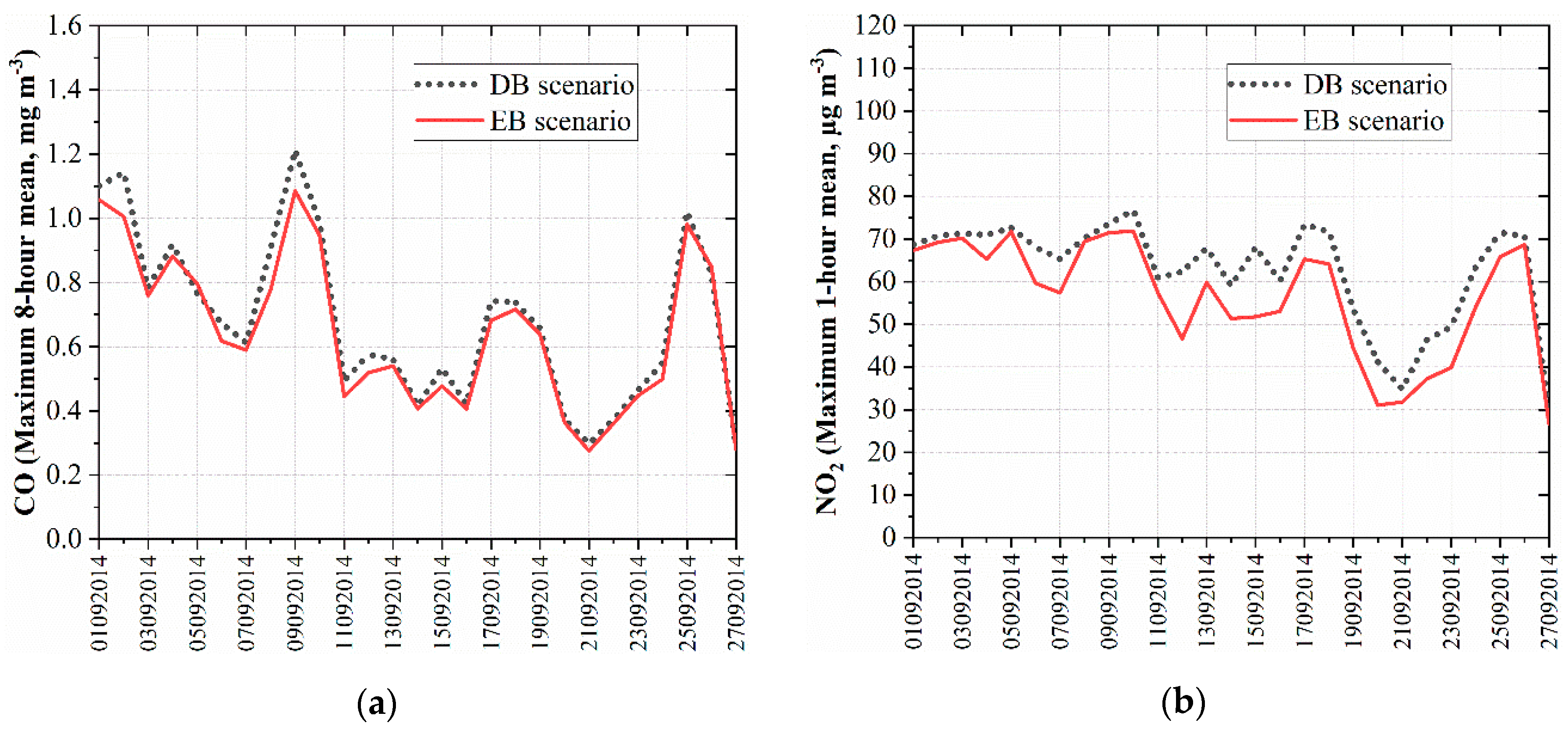
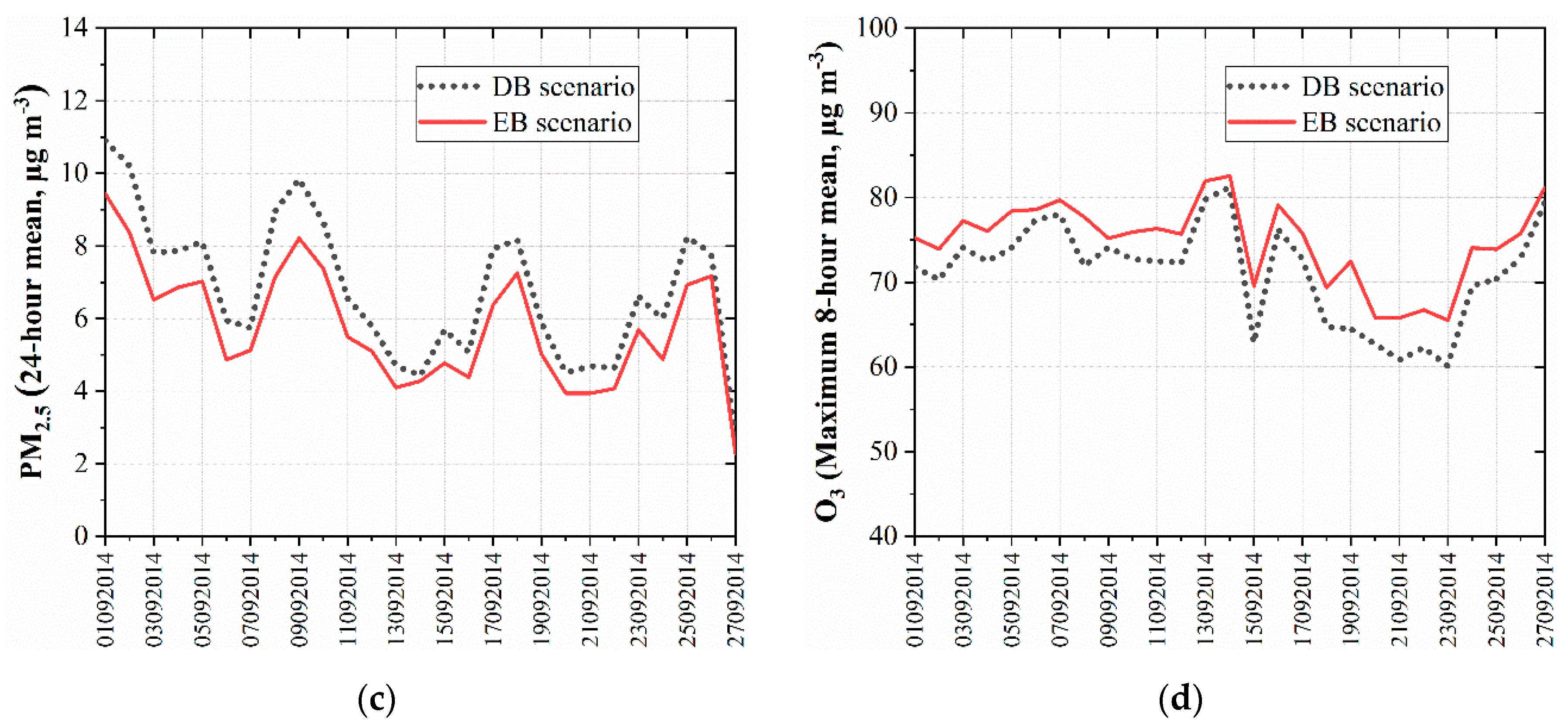
At the location of the MUN station, differences between the simulated scenarios (DB - EB) showed decreases in CO (between 0.00 and 0.14 mg m−3, median 0.02 mg m−3), NO2 (0.8 to 16.4 µg m−3, median 7.1 µg m−3), and 24-h mean PM2.5 (0.2 to 1.8 µg m−3, median 0.9 µg m−3) concentrations. However, the maximum 8-h mean O3 increased (1.1 to 8.0 µg m−3, median 3.5 µg m−3) (Figure 4).
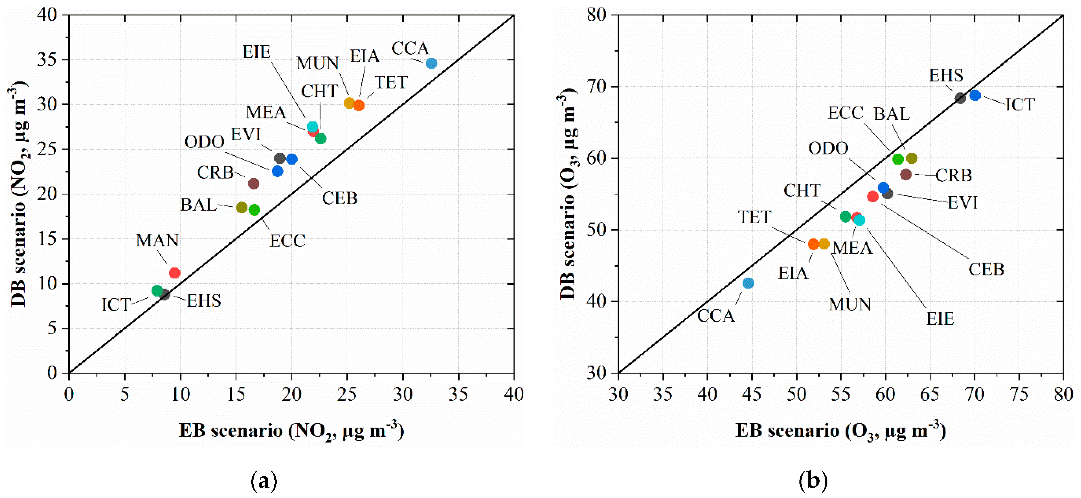
At the passive stations, the results of EB compared to the DB scenario (Figure 5) showed decreases in mean-monthly NO2 (0.2 to 5.6 µg m−3, median 3.8 µg m−3), although increases in mean-monthly O3 (0.0 to 5.7 µg m−3, median 3.9 µg m−3) (Figure 5). The smallest differences, for both NO2 and O3, were computed at Ictocruz (ICT) and Escuela Héctor Sempértegui (EHS), which are passive stations located in the south and north, respectively, in terms of the consolidated urban area of Cuenca (Figure 1), and, therefore, are only influenced by on-road traffic emissions to a small degree.
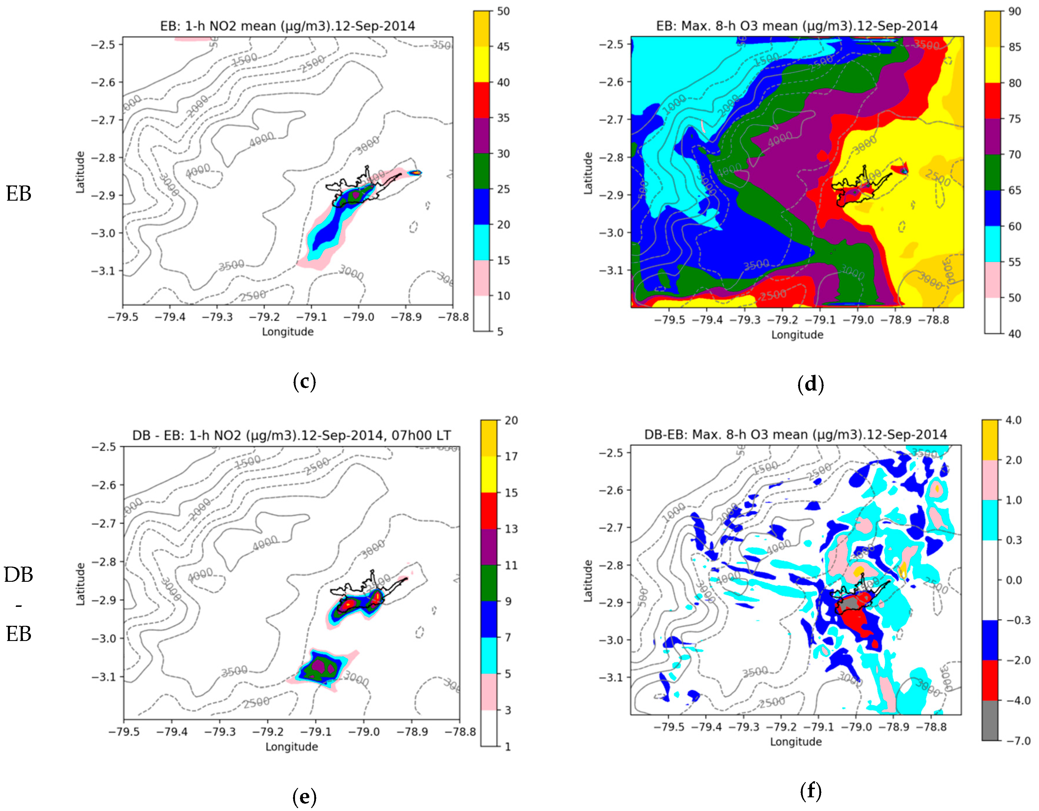
Figure 6 shows the modeled maps of NO2 (1-h mean at 7:00 local time (LT)) and O3 (maximum 8-h mean) concentrations of the DB and EB scenarios, from 12 September 2014. The Supplementary Materials section shows movies of the hourly modeled concentrations of NO2 and O3 from 12 September 2014, for both the DB and EB scenarios.
For the DB scenario, NOx (NO2 concentrations up to 45 µg m−3) in the urban area titrate O3, reducing its concentrations (up to about 75 µg m−3) compared to the levels computed for surrounding zones of the urban area (up about 85 µg m−3). For the EB scenario, NOx (NO2 concentrations up to 35 µg m−3) titrate to a lower degree, allowing higher O3 concentrations (up to about 80 µg m−3) in the urban area of Cuenca. When shifting to the EB scenario, modeled differences showed NO2 decreases between 3 and 15 µg m−3, and O3 increases between 3 and 7 µg m−3.
The modeled results indicate that the primary benefits of shifting from diesel to electric buses, as a mandatory action established in the Ecuadorian efficiency law, are decreases in the maximum 1-h mean NO2 (median 7.1 µg m−3) and the 24-h mean PM2.5 (median 0.9 µg m−3). However, this shift can increase the maximum 8-h mean O3 concentrations (median 3.5 µg m−3).
Apart from decreasing their short-term concentrations, lowering the NO2 and PM2.5 will also reduce their annual mean levels, promoting the attainment of the WHO guidelines and the air quality regulation. We highlight the benefits of reducing air pollution and particulate matter, owing to their carcinogenicity to humans [12,13], and the effects of particulate matter on the brain, which, according to recent literature, is the component of air pollution that appears to be the most concerning [17]. The modeled results and VOC-limited regime for photochemical O3 production suggest that VOC controls should accompany future NOx reduction to avoid an increase in O3 levels in the urban area of Cuenca.
In the future, the RTV should incorporate both NOx and VOC emission controls to verify the proper condition of exhaust catalysts for gasoline cars. Additionally, the RTV should incorporate NOx and PM2.5 controls for diesel vehicles.
The direction of change in pollutants between the DB and EB scenarios was consistent with that observed during the COVID-19 lockdown. Although other sources reduced their activities, the absence of buses allowed, to a high degree, a reduction in NOx and PM2.5 in the urban area of Cuenca. This consistency supports the validity of the approach used in this contribution to assess the effects of the future shift from diesel to electric buses in Cuenca.
The modeled results provide a preliminary estimation of air quality benefits based on the assumption that all diesel buses belonging to public transportation in the future will be replaced by electric buses. An updated emission inventory and the proposal of an appropriate future electric bus fleet (electric and hybrid) configuration will refine these results. Another limitation of our study is the period employed for modeling. Although September was considered representative, it is advisable to model other months or even the entire yearly period.
Another scenario deserving exploration is the control of emissions from heavy diesel vehicles, which contributed the largest percentages of on-road emissions of NOx (36.9%) and PM2.5 (63.4%) in 2014. The effects of NMVOC controls should be explored for gasoline cars, especially for older vehicles. Due to their emissions, other sources deserving dedicated assessments are industrial activities, the power facility, and the handcrafted production of bricks.
The operation of the tram project will produce changes in the public transportation system of Cuenca. The routes of buses need to be appropriately redesigned to define the best way to incorporate them. Emissions from buses will be redistributed, alleviating their magnitude on the historic center, although moving emissions to areas under the influence of new routes.
Table 4 presents a comparison with other assessments on the influence of moving to electric vehicles. Minet et al. (2020) [43] and Soret et al. (2014) [44], although using WRF as the meteorological model, used Polair3D and the Community Multiscale Air Quality Model (CMAQ) as the chemical transport model when studying the effects on the air quality in areas of Canada and Spain, respectively. Minet et al. (2020) reported decreases in NO2 and PM2.5, although they did not focus on O3. In agreement with the tendencies of our modeled results, Soret et al. (2014) reported decreases in NO2 and PM2.5, but increases in O3. One advantage of using WRF-Chem is the possibility to apply an online approach, allowing simultaneous treatment with feedback between meteorological and air quality variables.
Nogueira et al. (2019) [45] and Varga et al. (2019) [46] applied an approach based on changes in emissions when assessing the effects in São Paulo (Brazil) and Cluj-Napoca (Romania), respectively. These assessments, summarized in Table 4, reported decreases in NOx emissions.
Although the replacement of diesel buses by electric buses will reduce the emissions along the routes used by these vehicles, the generation of electricity will produce air pollution in the areas of influence of the fossil fuel power facilities belonging to the Ecuadorian mix. From 2001 to 2018, electricity came from renewable sources (43.5% to 73.6%), fossil fuels (26.2% to 52.2%), and importations (0.1% to 11.5%) [47]. Non-renewable sources include the combustion of fuel oil, diesel, naphtha, natural gas, bunker, oil, and liquid petroleum gas. The impact on air quality due to the electricity produced in Ecuador is a topic deserving of further research.
3.3. Air Quality during the COVID-19 Lockdown
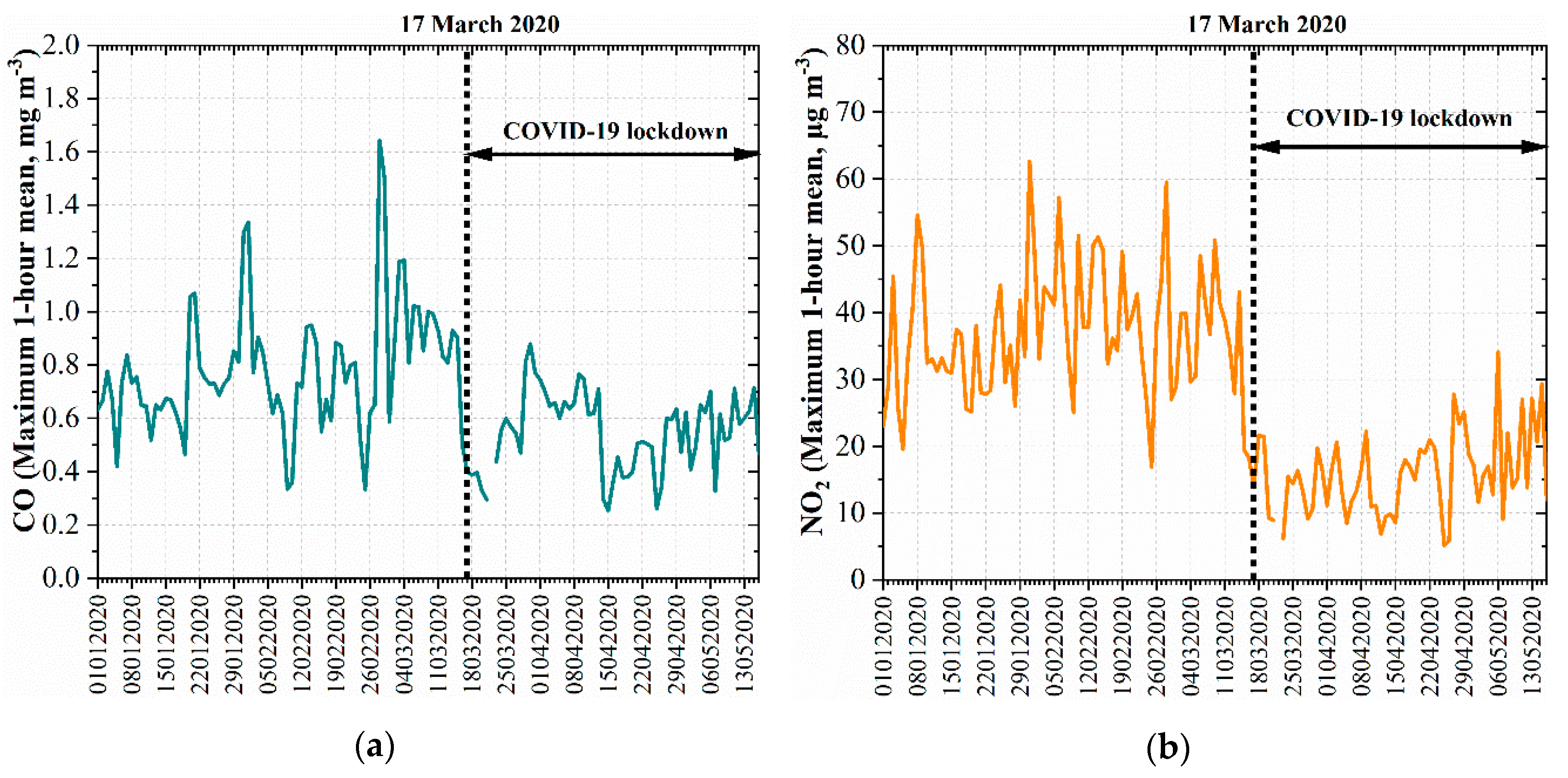
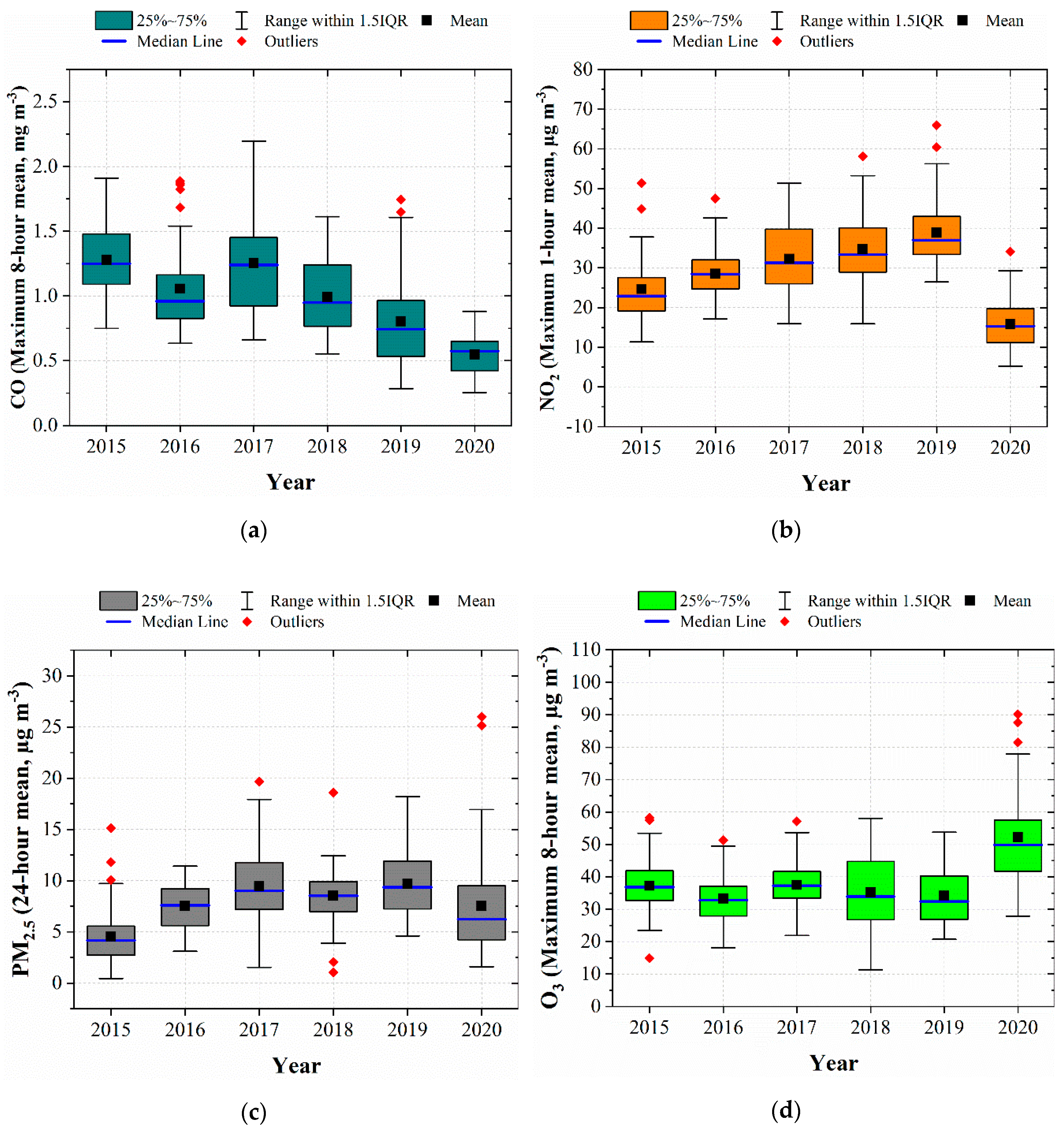
The concentrations of CO and NO2 were lower during the COVID-19 lockdown compared to previous records from 2020 (Figure 7). The maximum 8-h mean CO mean decreased from 0.74 (median) to 0.60 mg m−3. The maximum 1-h mean NO2 decreased from 36.8 (median) to 16.3 µg m−3. The distributions of CO and NO2 during the lockdown period were statistically different, with lower levels compared to distributions from 01 January 2020 to 16 March 2020 (Table 5).
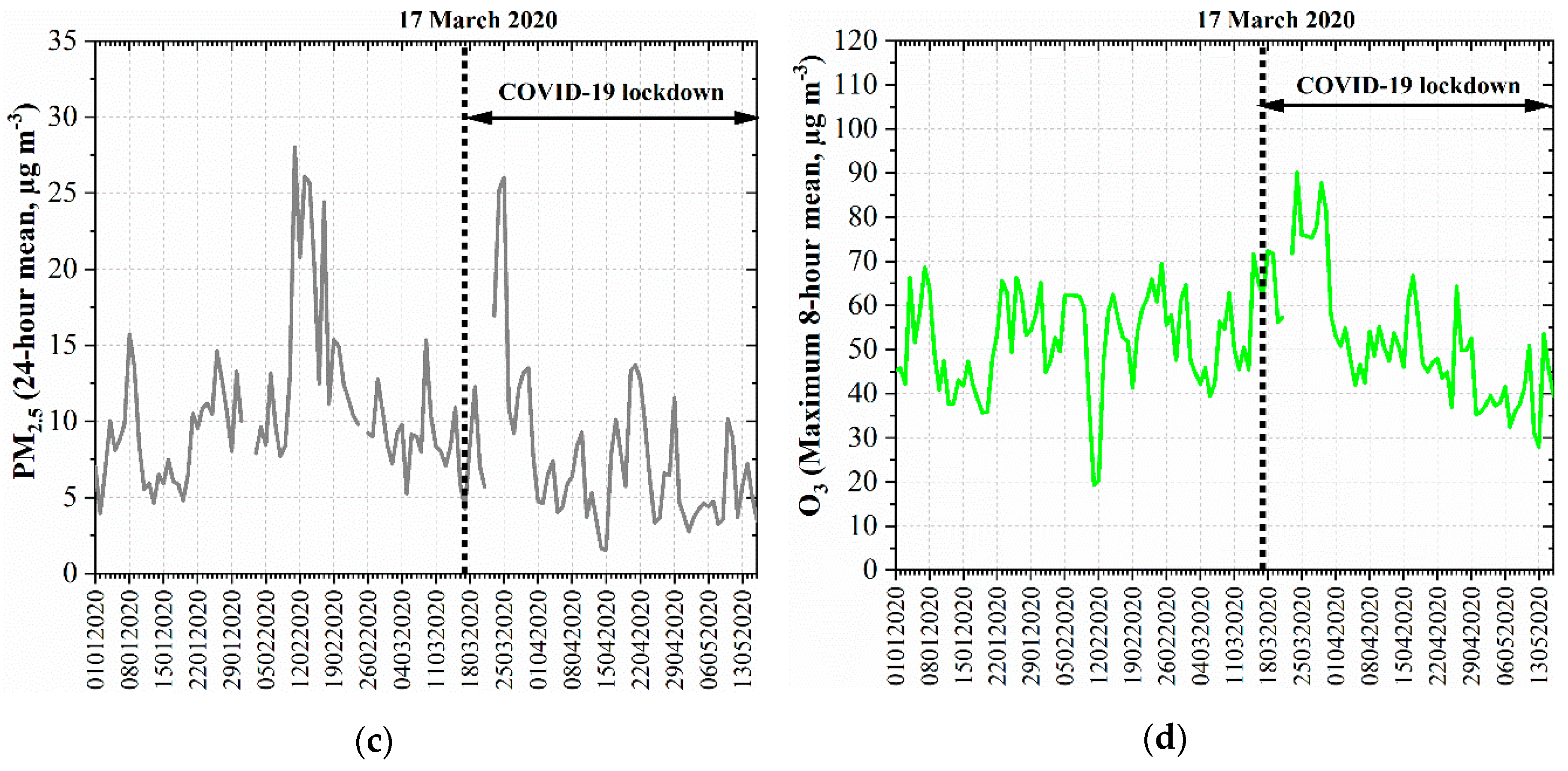
Additionally, the concentrations of PM2.5 were lower during the restriction (Figure 7). The 24-h mean PM2.5 decreased from 9.6 (median) to 5.7 µg m−3. The peak after 17 March 2020 can be associated with the arrival of volcanic ash from the Cayambe—one of the currently active volcanoes in Ecuador [48]—which produced light ash fallout in Cuenca on 24 March 2020 [49]. This peak influenced the PM2.5 records from 17 March to 16 April 2020, which showed a distribution statistically equal to records from 01 January to 16 March 2020.
During the first days of the lockdown, the O3 concentrations increased. The maximum 8-h mean O3 rose from 52.2 to 55.7 µg m−3, with the last value being the median from the first month after 17 March 2020. The median from 17 March 2020 to 16 May 2020 was 47.1 µg m−3. The distribution of O3 from 17 March to 16 April 2020 was statistically different, showing higher values compared to the distribution from 01 January to 16 March 2020 (Table 4). However, the distribution of O3 from 17 March to 16 May 2020 was statistically equal, showing similar levels to the distribution from 01 January to 16 March 2020.
The seasonal behavior of the maximum 8-h mean O3 in Cuenca shows a decrease during April and May, with the lowest concentrations during June and July (Figure 8). After this, O3 increases, typically reaching the highest values during September. Therefore, the O3 decrease during the second month of the lockdown relates to its seasonal variation. Figure 8 shows that the O3 levels during the COVID-19 lockdown were higher than the concentrations from previous years (2015 to 2019).
Figure 8 shows the mean profile (maximum 8-h mean) of O3 concentrations deduced from the records of the period 2015 to 2019 and the concentrations from 2020. The profile from 2020 shows, in general, higher concentrations compared to the mean of the previous years. From 01 January to 16 March, the O3 concentrations from 2020 were 10.0 µg m−3 (median) higher than the mean profile from previous years. During the lockdown (17 March to 16 May 2020), this difference increased to 13.9 µg m−3 (median), indicating a net increase of 3.9 µg m−3, which is consistent with the increase (3.5 µg m−3, median) obtained by modeling when assessing the air quality effects of moving from DB to EB.
Figure 9 compares the records from the lockdown to previous years. The median values of CO, NO2, PM2.5, and O3 from 2015 to 2019 varied between 0.74 and 1.24 mg m−3, 22.9 and 37.0 µg m−3, 4.2 and 9.4 µg m−3, and 32.4 and 37.3 µg m−3, respectively. During the COVID-19 lockdown, the medians of CO and NO2 dropped to 0.57 mg m−3 and 15.3 µg m−3, respectively. The PM2.5 during 2020 was 6.2 µg m−3, so it was higher than the value from 2015. However, O3 during 2020 increased to 49.8 µg m−3.
The distributions of CO and NO2 during the lockdown period from 2020 were statistically different, showing lower concentrations compared to the distributions of the same period from 2015 to 2019 (Table 6). Similarly, the distribution of O3 was statistically different, showing higher levels compared to the previous years. The distribution of PM2.5 during the lockdown period from 2020 was statistically equal, only showing similar concentrations to 2016.
The low PM2.5 median from 2015 (4.2 µg m−3) can be associated with the reduction in traffic—especially buses—in the historic center, due to activities of the construction of the electric tram. This project’s construction activities caused the closing of streets and changes in the routes of buses and limited the use of particular vehicles [28]. The operation of this project will produce changes in the public transportation system of Cuenca. At the time of writing this manuscript, the tram was being tested, and it will officially start working during the upcoming weeks.
The decrease in CO, NO2, and PM2.5 from 17 March to 16 May 2020, compared to previous weeks (01 January to 16 March 2020), was consistent with the decrease of these pollutants compared to previous years (2015 to 2019). Although other activities, such as some industries, probably reduced their activities, these changes can be associated, to a high degree, with reductions in on-road traffic. During the restriction, all types of vehicles reduced their activity. Buses did not work, and, therefore, there were essential reductions in NO2 and PM2.5.
On the other hand, the increase in O3 concentrations is consistent with the hypotheses behind the WE [50]. Among them, the results suggested that the following could have a leading role:
- There is a VOC-limited regime, with a VOC/NOx ratio lower than 8. Under this regime, VOC limits O3 production, and NOx reduction promotes O3 production, and;
- Less O3 is titrated because NOx emissions are lower compared to weekdays.
Other mechanisms, such as the reduction in soot, can contribute to higher O3 concentrations. More studies are required to define the participation of these and other hypotheses behind the WE in Cuenca.
Figure 10 shows the mean profiles of global solar radiation from 2017 to 2020 (MUN station), corresponding to the period 17 March to 16 May. These profiles indicate the mean levels of solar radiation from 9:00 to 16:00, representing the hours when O3 concentrations are typically higher. The profile of 2020 did not show higher values compared to previous years. The corresponding Wilcoxon tests indicated that the distributions of global radiation records from 2020 were statistically equal compared to the previous three years. These results indicate that the increase in O3 concentrations during 2020 is not related to higher solar radiation levels. Apart from changes in the emissions of precursors, another factor potentially involved is the long-range transport of O3. From 1 January to 16 May of 2020, Terra and Aqua satellites [51] identified forest fires, mainly in Colombia and Venezuela, toward the northeast of Ecuador. In addition, forest fires were mostly identified in the north of Peru and the center of Brazil. At the latitude of Cuenca, forest fires were less abundant and mainly at the center and west of South America. Although the influence of forest fires is outside the scope of this study, their occurrence from 1 January to 16 May suggests their emissions were not the leading cause of O3 increases during the COVID-19 lockdown.
The effects of the COVID-19 lockdown and modeled results presented in this contribution provide an early reference for the potential changes in the air quality of Cuenca during the next few years.
4. Conclusions and Summary
Based on records from seven years (2013 to 2019), we confirmed the presence of the WE in the urban area of Cuenca, where on-road traffic is the most relevant air pollutant source. The VOC-limited regime for O3 production explains, at least in part, the mean increase in O3 concentrations during weekends, despite the decreased emissions of NOx and VOC, in comparison to weekdays. This regime is behind a counterintuitive variation of O3 owing to the variation of NOx emissions: The increase in NOx emissions decreases O3 concentrations, and the decrease in NOx emissions increases the O3 levels.
Our preliminary assessment, based on the assumption that all diesel buses will be replaced by electric buses, implies the elimination of 1861.2 t y−1 of NOx and 81.7 t y−1 of PM2.5 exhaust emissions (Table 2). The modeled results indicated decreases in NO2 and PM2.5 but increases in O3 concentrations. The direction of these changes was consistent with the VOC-limited regime presented in Cuenca.
The effects of the limitation of activities during the COVID-19 lockdown also showed consistent variations (NO2 decrease and O3 increase) in comparison to the VOC-limited regime for O3 production.
There was consistency between the WE, the effects on air quality during the COVID-19 lockdown, and the modeled results owing to the future shift in the public transportation system of Cuenca. This consistency supports the modeling approach used in this contribution for assessing future air quality scenarios, owing to changes in the emission inventories. The same approach can be used to assess the effects of reductions in other emission sources, such as old gasoline cars (high NMVOC emissions). Moreover, the modeled results and their consistency with the WE and the effects of the COVID-19 lockdown support the validity of the emission inventory from 2014, which, although not a recent one, is a useful component for modeling purposes. Future emissions inventories should follow the same approach used when building the emission inventory from 2014.
Our findings suggest that VOC emission controls should accompany a future reduction in NOx emissions to avoid an increase in O3 levels in the urban area of Cuenca. In the future, the RTV should incorporate both NOx and VOC emission controls to verify the proper condition of exhaust catalysts for gasoline cars. Furthermore, the RTV should incorporate NOx and PM2.5 controls for diesel vehicles.
The operation of the electric tram system will produce changes in the transportation system of Cuenca. Emissions from buses will be redistributed, alleviating their magnitude in the historic center. The effects of the COVID-19 lockdown and modeled results presented in this contribution provide an early reference for the potential changes in the air quality of Cuenca during the upcoming years, due to the recent operability of the electric tram and the future shift from diesel to electric buses in Cuenca.
Supplementary Materials
The following are available online at https://0-www-mdpi-com.brum.beds.ac.uk/2073-4433/11/9/998/s1, Movies of the hourly modeled maps of NO2 (12-Sep-2014_NO2_DB, 12-Sep-2014_NO2_EB) and O3 (12-Sep-2014_O3_DB, 12-Sep-2014_O3_EB) from 12-Sep-2014.
Author Contributions
Conceptualization, methodology, modeling, validation, formal analysis, and writing—review and editing, R.P.; passive monitoring, laboratory analysis, data processing, and curation, C.E. All authors have read and agreed to the published version of the manuscript.
Acknowledgments
This research is part of the project “Emisiones y Contaminación Atmosférica en el Ecuador 2020-2021”. Simulations were done on the High-Performance Computing system at the USFQ.
Funding
This research received no external funding.
Conflicts of Interest
The authors declare no conflict of interest.
References
- Ministerio del Ambiente. Inventario de Emisiones de contaminantes del aire para los cantones Esmeraldas, Ibarra, Santo Domingo, Manta, Portoviejo, Milagro, Riobamba, Ambato y Latacunga, Año Base 2010; Ministerio del Ambiente: Quito, Ecuador, 2012.
- Ministerio del Ambiente. Inventario de Emisiones de contaminantes del aire para los cantones Loja, Azogues, Babahoyo y Quevedo, Año Base: 2010; Ministerio del Ambiente: Quito, Ecuador, 2013. [Google Scholar]
- Molina, M.; Molina, L. Megacities and Atmospheric Pollution. Critical review. J. Air Waste Manag. Assoc. 2004, 54, 644–680. [Google Scholar] [CrossRef] [PubMed]
- EMOV EP. Inventario de Emisiones Atmosféricas del Cantón Cuenca 2014; Empresa Pública de Movilidad: Tránsito y Transporte, Cuenca, Ecuador, 2016; 86p. [Google Scholar]
- Lloyd, A.C.; Cackette, T.A. Diesel engines: Environmental impact and control. J Air Waste Manag. Assoc. 2001, 51, 809–847. [Google Scholar] [CrossRef] [PubMed] [Green Version]
- Jacobson, M.Z. Atmospheric Pollution History, Science and Regulation; University Press: Cambridge, UK, 2002; p. 399. [Google Scholar]
- Biswas, P.; Wu, C.Y. Nanoparticles and the environment. J Air Waste Manag. Assoc. 2005, 55, 708–746. [Google Scholar] [CrossRef] [PubMed]
- Finlayson, B.J.; Pitts, J., Jr. Tropospheric air pollution: Ozone, airborne toxics, polycyclic aromatic hydrocarbons, and particles. Science 1997, 276, 1046–1051. [Google Scholar] [CrossRef] [PubMed] [Green Version]
- WHO. Air Quality Guidelines for Europe, Second Edition. World Health Organization Regional Publications, European Series; WHO: Geneva, Switzerland, 2000; No. 91. [Google Scholar]
- Phalen, R. Introduction to Air Pollution Science—A Public Health Perspective, Science and Regulation; Jones & Bartlett Learning: Burlington, LA, USA, 2013; p. 331. [Google Scholar]
- WHO. WHO Air Quality Guidelines for Particulate Matter, Ozone, Nitrogen Dioxide and Sulfur Dioxide. Global update 2005. Summary of Risk Assessment; WHO: Geneva, Switzerland, 2006. [Google Scholar]
- IARC. International Agency for Research on Cancer. Available online: https://publications.iarc.fr/538 (accessed on 13 August 2020).
- Loomis, D.; Grosse, Y.; Lauby-Secretan, B.; El Ghissassi, F.; Bouvard, V.; Benbrahim-Tallaa, L.; Guha, N.; Baan, R.; Mattock, H.; Straif, K. The carcinogenicity of outdoor air pollution. Lancet Oncol. 2013, 14, 1262–1263. [Google Scholar] [CrossRef]
- Calderón-Garcidueñas, L.; Gónzalez-Maciel, A.; Reynoso-Robles, R.; Delgado-Chávez, R.; Mukherjee, P.S.; Kulesza, R.J.; Torres-Jardón, R.; Ávila-Ramírez, J.; Villarreal-Ríos, R. Hallmarks of Alzheimer disease are evolving relentlessly in Metropolitan Mexico City infants, children and young adults. APOE4 carriers have higher suicide risk and higher odds of reaching NFT stage V at ≤40 years of age. Environ. Res. 2018, 164, 475–487. [Google Scholar] [CrossRef]
- Cacciottolo, M.; Wang, X.; Driscoll, I.; Woodward, N.; Saffari, A.; Reyes, J.; Serre, M.L.; Vizuete, W.; Sioutas, C.; E Morgan, T.; et al. Particulate air pollutants, APOE alleles and their contributions to cognitive impairment in older women and to amyloidogenesis in experimental models. Transl. Psychiatry 2017, 7, e1022. [Google Scholar] [CrossRef]
- Austin, W.; Heutel, G.; Kreisman, D. School bus emissions, student health and academic performance. Econ. Educ. Rev. 2019, 70, 109–126. [Google Scholar] [CrossRef]
- Peeples, L. News Feature: How air pollution threatens brain health. Proc. Natl. Acad. Sci. USA 2020, 117, 13856–13860. [Google Scholar] [CrossRef]
- Parra, R. Performance studies of planetary boundary layer schemes in wrf-chem for the andean region of southern ecuador. Atmos. Pollut. Res. 2018, 9, 411–528. [Google Scholar] [CrossRef]
- Baklanov, A.; Schlünzen, K.; Suppan, P.; Baldasano, J.; Brunner, D.; Aksoyoglu, S.; Carmichael, G.; Douros, J.; Flemming, J.; Forkel, R.; et al. Online coupled regional meteorology chemistry models in Europe: Current status and prospects. Atmos. Chem. Phys. 2014, 14, 317–398. [Google Scholar] [CrossRef] [Green Version]
- EMOV EP. Informe de calidad del aire Cuenca 2019. Alcaldía de Cuenca. Red de Monitoreo EMOV EP. Cuenca-Ecuador; EMOV EP: Cuenca, Ecuador, 2020; 114p. [Google Scholar]
- EMOV EP. Informe de calidad del aire Cuenca 2013. Alcaldía de Cuenca. Red de Monitoreo EMOV EP. Cuenca-Ecuador; EMOV EP: Cuenca, Ecuador, 2014; 100p. [Google Scholar]
- EMOV EP. Informe de calidad del aire Cuenca 2014. Alcaldía de Cuenca. Red de Monitoreo EMOV EP. Cuenca-Ecuador; EMOV EP: Cuenca, Ecuador, 2015; 97p. [Google Scholar]
- EMOV EP. Informe de calidad del aire Cuenca 2015. Alcaldía de Cuenca. Red de Monitoreo EMOV EP. Cuenca-Ecuador; EMOV EP: Cuenca, Ecuador, 2016; 120p. [Google Scholar]
- EMOV EP. Informe de calidad del aire Cuenca 2016. Alcaldía de Cuenca. Red de Monitoreo EMOV EP. Cuenca-Ecuador; EMOV EP: Cuenca, Ecuador, 2017; 103p. [Google Scholar]
- EMOV EP. Informe de calidad del aire Cuenca 2017. Alcaldía de Cuenca. Red de Monitoreo EMOV EP. Cuenca-Ecuador; EMOV EP: Cuenca, Ecuador, 2018; 121p. [Google Scholar]
- EMOV EP. Informe de calidad del aire Cuenca 2018. Alcaldía de Cuenca. Red de Monitoreo EMOV EP. Cuenca-Ecuador; EMOV EP: Cuenca, Ecuador, 2019; 107p. [Google Scholar]
- Parra, R. Efecto Fin de Semana en la Calidad del Aire de la Ciudad de Cuenca, Ecuador. ACI Av. Cienc. Ing. 2017, 9, 104–111. [Google Scholar] [CrossRef] [Green Version]
- Rumé, S. Reflexiones antropológicas sobre la difícil ejecución del proyecto tranvía en Cuenca. Revista Interuniversitaria de Estudios Urbanos de Ecuador 2018, 4, 25–34. [Google Scholar]
- Ministerio de Energía y Recursos Naturales No Renovables. Available online: https://www.recursosyenergia.gob.ec/wp-content/uploads/downloads/2019/03/Ley-Eficiencia-Energe%CC%81tica.pdf (accessed on 13 June 2020).
- Nakada, L.Y.; Urban, R.C. COVID-19 pandemic: Impacts on the air quality during the partial. Sci. Total Environ. 2020, 730, 1–5. [Google Scholar] [CrossRef] [PubMed]
- Jia, C.; Fu, X.; Bartelli, D.; Smith, L. Insignificant impact of the “Stay-At-Home” order on ambient air quality in the memphis metropolitan area, U.S.A. Atmosphere 2020, 11, 630. [Google Scholar] [CrossRef]
- Sicard, P.; De Marco, A.; Agathokleous, E.; Feng, Z.; Xu, X.; Paolettie, E.; Diéguez, J.J.; Calatayud, V. Amplified ozone pollution in cities during the COVID-19 lockdown. Sci. Total Environ. 2020, 735, 1–10. [Google Scholar] [CrossRef]
- Otmani, A.; Benchrif, A.; Tahri, M.; Bounakhla, M.; Chakir, E.M.; Bouch, M.E.; Krombi, M. Impact of Covid-19 lockdown on PM10, SO2 and NO2 concentrations in Salé City (Morocco). Sci. Total Environ. 2020, 735, 1–5. [Google Scholar] [CrossRef]
- Presidencia de la República del Ecuador. Consultas de Decretos. 2020. Available online: https://minka.presidencia.gob.ec/portal/usuarios_externos.jsf (accessed on 13 June 2020).
- El Mercurio. Hay Nuevas Reglas Para Circulación en Cuenca. Available online: https://ww2.elmercurio.com.ec/2020/05/31/hay-nuevas-reglas-para-circulacion-en-cuenca/ (accessed on 13 June 2020).
- Seguel, R.; Morales, S.; Leiva, M. Ozone weekend effect in Santiago, Chile. Environ. Pollut. 2012, 162, 72–79. [Google Scholar] [CrossRef]
- Parra, R.; Franco, E. Identifying the Ozone Weekend Effect in the air quality of the northern Andean region of Ecuador. Wit Trans. Ecol. Environ. 2016, 207, 169–180. [Google Scholar]
- WRF. Weather Research and Forecasting Model. Available online: https://www.mmm.ucar.edu/weather-research-and-forecasting-model (accessed on 13 June 2020).
- NCEP. NCEP FNL Operational Model Global Tropospheric Analyses, Continuing from July 1999. Available online: https://rda.ucar.edu/datasets/ds083.2/ (accessed on 13 June 2020).
- Zaveri, R.; Peters, L. A new lumped structure photochemical mechanism for large-scale applications. J. Geophys. Res. 1999, 104, 387–415. [Google Scholar] [CrossRef]
- Zaveri, R.; Easter, R.; Fast, J.; Peters, L. Model for simulating aerosol interactions and chemistry (MOSAIC). J. Geophys. Res. 2008, 113, 1–29. [Google Scholar] [CrossRef]
- Skamarock, W.; Klemp, J.; Dudhia, J.; Barker, D.; Duda, M.; Huang, X.; Wang, W.; Powers, J. A Description of the Advanced Research WRF Version 3. NCAR/TN-475+STR. NCAR Technical Note. Mesoscale and Microscale Meteorology Division; National Center for Atmospheric Research: Boulder, CO, USA, 2008. [Google Scholar]
- Minet, L.; Chowdhury, T.; Wang, A.; Gai, Y.; Daniel Posen, I.; Roorda, M.; Hatzopoulou, M. Quantifying the air quality and health benefits of greening freight movements. Environ. Res. 2020, 183, 109193. [Google Scholar] [CrossRef]
- Soret, A.; Guevara, M.; Baldasano, J.M. The potential impacts of electric vehicles on air quality in the urban areas of Barcelona and Madrid (Spain). Atmos. Environ. 2014, 99, 51–63. [Google Scholar] [CrossRef]
- Nogueira, T.; Dominutti, P.A.; Vieira-Filho, M.; Fornaro, A.; Andrade, M.F. Evaluating Atmospheric Pollutants from Urban Buses under Real-World Conditions: Implications of the Main Public Transport Mode in São Paulo, Brazil. Atmosphere 2019, 10, 108. [Google Scholar] [CrossRef] [Green Version]
- Varga, B.O.; Mariasiu, F.; Miclea, C.D.; Szabo, I.; Sirca, A.A.; Nicolae, V. Direct and Indirect Environmental Aspects of an Electric Bus Fleet Under Service. Energies 2020, 13, 336. [Google Scholar] [CrossRef] [Green Version]
- Parra, R. Contribution of Non-renewable Sources for Limiting the Electrical CO2 emission factor in Ecuador. WIT Trans. Ecol. Environ. 2020, 244, 65–77. [Google Scholar]
- Bernard, B.; Battaglia, J.; Proaño, A.; Hidalgo, S.; Vásconez, F.; Hernandez, S.; Ruiz, M. Relationship between volcanic ash fallouts and seismic tremor: Quantitative assessment of the 2015 eruptive period at Cotopaxi volcano, Ecuador. Bull. Volcanol. 2016, 78, 80. [Google Scholar] [CrossRef]
- El Mercurio. Cenizas del Volcán Sangay Cayeron Sobre Cuenca de Forma Leve. Available online: https://ww2.elmercurio.com.ec/2020/03/25/cenizas-del-volcan-sangay-caen-sobre-cuenca-de-forma-leve/ (accessed on 17 June 2020).
- CARB. The ozone weekend effect in California. In Staff Report, the Planning and Technical Support Division, the Research Division, Air Resources Board, California Environmental Protection Agency; CARB: Sacramento, CA, USA, 2003. [Google Scholar]
- Worldview. Available online: https://worldview.earthdata.nasa.gov/ (accessed on 9 September 2020).
Figure 1.
Location of: (a) Ecuador and (b) Cuenca. (c) PM2.5 emissions (t y−1). (d) Urban area of Cuenca and the air quality stations (red dots). MUN station (2500 m. a.s.l.) provides short-term air quality levels and meteorology. The others are passive stations for monitoring monthly-mean air quality concentrations. Nomenclature of stations: MUN, Municipio; EHS, Escuela Héctor Sempértegui; ECC, Escuela Carlos Crespi; CCA, Colegio Carlos Arízaga; MAN, Machángara; CEB, Cebollar; BAL, Balzay; VEG, Vega Muñoz; TET, Terminal Terrestre; EIA, Escuela Ignacio Andrade; MEA, Mercado El Arenal; BCB, Bomberos; CHT, Colegio Herlinda Toral; LAR, Calle Larga; MIS, Misicata; CRB, Colegio Rafael Borja; EIE, Escuela Ignacio Escandón; EVI, Escuela Velasco Ibarra; ODO; Facultad de Odontología; ICT, Ictocruz.

Figure 2.
Mean-daily profiles from 2018: (a) CO, (b) NO2, (c) PM2.5, and (d) ozone (O3).

Figure 3.
Increase in the maximum 8-h mean O3 concentrations from Saturdays and Sundays compared to weekdays. Period of 2013 to 2019.
Figure 3.
Increase in the maximum 8-h mean O3 concentrations from Saturdays and Sundays compared to weekdays. Period of 2013 to 2019.

Figure 4.
Modeled concentrations from September 2014 for the scenarios DB (diesel buses) and EB (electric buses). (a) Maximum 8-h mean CO, (b) maximum 1-h mean NO2, (c) 24 h mean PM2.5, and (d) maximum 8-h O3 mean.
Figure 4.
Modeled concentrations from September 2014 for the scenarios DB (diesel buses) and EB (electric buses). (a) Maximum 8-h mean CO, (b) maximum 1-h mean NO2, (c) 24 h mean PM2.5, and (d) maximum 8-h O3 mean.


Figure 5.
Comparison of modeled mean-monthly concentrations of September 2014. Horizontal axis: EB (electric buses) scenario. Vertical axis: DB (diesel buses) scenario. (a) NO2 and (b) O3. Nomenclature corresponds to the passive stations.
Figure 5.
Comparison of modeled mean-monthly concentrations of September 2014. Horizontal axis: EB (electric buses) scenario. Vertical axis: DB (diesel buses) scenario. (a) NO2 and (b) O3. Nomenclature corresponds to the passive stations.

Figure 6.
Modeled NO2 (1-h mean at 7:00 LT): (a) DB, (c) EB, and (e) DB − EB. Modeled O3 (maximum 8-h mean): (b) DB, (d) EB, and (f) DB-EB. 12 September 2014.
Figure 6.
Modeled NO2 (1-h mean at 7:00 LT): (a) DB, (c) EB, and (e) DB − EB. Modeled O3 (maximum 8-h mean): (b) DB, (d) EB, and (f) DB-EB. 12 September 2014.


Figure 7.
Air quality in Cuenca from 01 January to 16 May 2020. (a) Maximum 8-h mean CO. (b) Maximum 1-h mean NO2. (c) 24-h mean PM2.5. (d) Maximum 8-h mean O3.
Figure 7.
Air quality in Cuenca from 01 January to 16 May 2020. (a) Maximum 8-h mean CO. (b) Maximum 1-h mean NO2. (c) 24-h mean PM2.5. (d) Maximum 8-h mean O3.


Figure 8.
(a) Maximum 8-h mean O3 from 2015 to 2020. (b) Mean maximum 8-h O3 from 2015 to 2019 and maximum 8-h O3 from 2020. Urban area (MUN station) of Cuenca.
Figure 8.
(a) Maximum 8-h mean O3 from 2015 to 2020. (b) Mean maximum 8-h O3 from 2015 to 2019 and maximum 8-h O3 from 2020. Urban area (MUN station) of Cuenca.

Figure 9.
Air quality in Cuenca (MUN station) from 17 March to 16 May from 2015 to 2020. (a) Maximum 8-h mean CO. (b) Maximum 1-h mean NO2. (c) 24-h mean PM2.5. (d) Maximum 8-h mean O3.
Figure 9.
Air quality in Cuenca (MUN station) from 17 March to 16 May from 2015 to 2020. (a) Maximum 8-h mean CO. (b) Maximum 1-h mean NO2. (c) 24-h mean PM2.5. (d) Maximum 8-h mean O3.

Figure 10.
Mean profiles of global solar radiation from 2017 to 2020 in the urban area (MUN station) of Cuenca. Period 17 March to 16 May.
Figure 10.
Mean profiles of global solar radiation from 2017 to 2020 in the urban area (MUN station) of Cuenca. Period 17 March to 16 May.


Table 1.
Summary of air pollutant emissions from Cuenca (Ecuador). Year 2014 [4].
Table 1.
Summary of air pollutant emissions from Cuenca (Ecuador). Year 2014 [4].
| Source | NOx | CO | NMVOC | SO2 | PM10 | PM2.5 | ||||||
|---|---|---|---|---|---|---|---|---|---|---|---|---|
| t y−1 | % | t y−1 | % | t y−1 | % | t y−1 | % | t y−1 | % | t y−1 | % | |
| On-road traffic | 5981.0 | 71.2 | 58,283.4 | 94.9 | 6065.4 | 39.6 | 67.9 | 4.0 | 800.2 | 55.6 | 384.0 | 42.4 |
| Vegetation | - | - | - | - | 2982.0 | 19.5 | - | - | - | - | - | - |
| Industries | 654.4 | 7.8 | 257.7 | 0.4 | 156.2 | 1.0 | 1025.9 | 60.4 | 73.1 | 5.1 | 52.1 | 5.7 |
| Power facility | 1553.8 | 18.5 | 334.4 | 0.5 | 126.8 | 0.8 | 595.0 | 35.1 | 102.1 | 7.1 | 102.1 | 11.3 |
| Use of solvents | - | - | - | - | 4551.7 | 29.7 | - | - | - | - | - | - |
| Service stations | - | - | - | - | 851.1 | 5.6 | - | - | - | - | - | - |
| Domestic GLP consumption | 137.9 | 1.6 | 21.5 | 0.0 | 4.6 | 0.0 | 0.0 | 0.0 | 9.1 | 0.6 | 9.1 | 1.0 |
| Air traffic | 24.2 | 0.3 | 36.0 | 0.1 | 5.4 | 0.0 | 4.3 | 0.3 | 0.3 | 0.0 | 0.3 | 0.0 |
| Landfills | - | - | - | - | 32.4 | 0.2 | - | - | - | - | - | - |
| Handcrafted production of bricks | 51.0 | 0.6 | 2465.4 | 4.0 | 534.2 | 3.5 | 4.1 | 0.2 | 353.4 | 24.6 | 349.3 | 38.5 |
| Dust erosion | - | - | - | - | - | - | - | - | 96.8 | 6.7 | 9.7 | 1.1 |
| Mining | - | - | - | - | - | - | - | - | 4.4 | 0.3 | 0.0 | 0.0 |
| Total | 8402 | 100 | 61,398 | 100 | 15,310 | 100 | 1697 | 100 | 1439 | 100 | 907 | 100 |
NOx: nitrogen oxides. CO: carbon monoxide. NMVOC: non-methane volatile organic compounds. SO2: sulfur dioxide. PM10: particulate matter with diameter ≤ 10 µm. PM2.5: particulate matter with diameter ≤ 2.5 µm.
Table 2.
Summary of air pollutant emissions from on-road traffic of Cuenca (Ecuador). Year 2014. Disaggregated emissions from diesel vehicles.
Table 2.
Summary of air pollutant emissions from on-road traffic of Cuenca (Ecuador). Year 2014. Disaggregated emissions from diesel vehicles.
| Pollutant | Unit | Gasoline Vehicles | Diesel Vehicles | Total | |||
|---|---|---|---|---|---|---|---|
| Automobile | Pick-Up | Bus | Heavy | ||||
| NOx | t y−1 | 1810.1 | 4.8 | 97.6 | 1861.2 | 2207.3 | 5981.0 |
| % | 30.3 | 0.1 | 1.6 | 31.1 | 36.9 | 100.0 | |
| CO | t y−1 | 52,429.8 | 12.0 | 340.5 | 2520.3 | 2980.8 | 58,283.4 |
| % | 90.0 | 0.0 | 0.6 | 4.3 | 5.1 | 100.0 | |
| NMVOC | t y−1 | 4417.2 | 3.9 | 97.5 | 693.4 | 853.6 | 6065.4 |
| % | 72.8 | 0.1 | 1.6 | 11.4 | 14.1 | 100.0 | |
| SO2 | t y−1 | 30.7 | 0.3 | 6.1 | 8.2 | 22.7 | 67.9 |
| % | 45.2 | 0.4 | 8.9 | 12.1 | 33.4 | 100.0 | |
| PM10 exhaust | t y−1 | 32.9 | 1.5 | 28.5 | 108.4 | 302.3 | 473.6 |
| % | 6.9 | 0.3 | 6.0 | 22.9 | 63.8 | 100.0 | |
| PM2.5 exhaust | t y−1 | 15.6 | 1.2 | 23.8 | 81.7 | 227.8 | 350.0 |
| % | 4.4 | 0.3 | 6.8 | 23.3 | 65.1 | 100.0 | |
| PM10 tire wear | t y−1 | 6.5 | 0.0 | 1.0 | 3.2 | 8.9 | 19.6 |
| % | 33.4 | 0.2 | 4.9 | 16.2 | 45.4 | 100.0 | |
| PM2.5 brake wear | t y−1 | 11.4 | 0.1 | 1.6 | 5.5 | 15.4 | 34.0 |
| % | 33.5 | 0.2 | 4.7 | 16.2 | 45.4 | 100.0 | |
| PM10 pavement | t y−1 | 13.7 | 0.1 | 2.0 | 4.6 | 12.9 | 33.3 |
| % | 41.2 | 0.2 | 6.0 | 13.8 | 38.7 | 100.0 | |
| PM10 resuspension | t y−1 | 189.1 | 1.0 | 20.5 | 16.6 | 46.5 | 273.7 |
| % | 69.1 | 0.4 | 7.5 | 6.1 | 17.0 | 100.0 | |
| PM10 Total | t y−1 | 242.3 | 2.6 | 52.0 | 132.8 | 370.6 | 800.2 |
| % | 30.3 | 0.3 | 6.5 | 16.6 | 46.3 | 100.0 | |
| PM2.5 Total | t y−1 | 26.9 | 1.2 | 25.4 | 87.2 | 243.3 | 384.0 |
| % | 7.0 | 0.3 | 6.6 | 22.7 | 63.4 | 100.0 | |
NOx: nitrogen oxides. CO: carbon monoxide. NMVOC: non-methane volatile organic compounds. SO2: sulfur dioxide. PM10: particulate matter with diameter ≤ 10 µm. PM2.5: particulate matter with diameter ≤2.5 µm. PM10 Total corresponds to the summation of PM10 exhaust, PM10 tire wear, PM10 pavement, and PM10 resuspension. PM2.5 Total corresponds to the summation of PM2.5 exhaust and PM2.5 brake wear. Gray background indicates the total values per pollutant.
Table 3.
Weather Research and Forecasting with Chemistry (WRF-Chem V3.2) physics parameterization for modeling the air quality in Cuenca [42].
Table 3.
Weather Research and Forecasting with Chemistry (WRF-Chem V3.2) physics parameterization for modeling the air quality in Cuenca [42].
| Component | Option | Scheme/Model |
|---|---|---|
| Microphysics | 4 | WRF Single–moment 5–class |
| Planetary Boundary Layer | 1 | Yonsei University (YSU) |
| Cumulus Parameterization | 5 | Grell 3D Ensemble |
| Shortwave | 2 | Goddard |
| Longwave | 1 | RRTM |
| Land Surface | 2 | Unified Noah Land Surface |
| Surface Layer | 1 | MM5 Similarity |
Table 4.
Comparison with other assessments on the influence of electric vehicles on air quality.
| Component | Case or Reference | ||||
|---|---|---|---|---|---|
| This Assessment | Minet et al. (2020) [43] | Soret et al. (2014) [44] | Nogueira et al. (2019) [45] | Varga et al. (2019) [46] | |
| Region | Cuenca, Ecuador | Toronto and Hamilton area, Canada | Barcelona and Madrid, Spain | São Paulo, Brazil | Cluj-Napoca, Romania |
| Period | September 2014 | 20 to 26 March and 14 to 20 August 2016 | 3 to 5 October 2011 | ||
| Approach | Emission changes and air quality modeling | Emission changes and air quality modeling | Emission changes and air quality modeling | Emission changes | Emission changes |
| Models | WRF-Chem | WRF, Polair3D | WRF, CMAQ | ||
| Spatial resolution | 1 km2 | 1 km2 | 1 km2 | ||
| Approach | Online | Offline | Offline | ||
| Main results reported | Decrease in NO2 (7.1 µg m−3) and PM2.5 (0.9 µg m−3) Increase in O3 (3.5 µg m−3) | Mean exposure decrease to NO2 (6% to 11%) and PM2.5 (9% to 13%) | Decrease in NO2 (35 µg m−3) and PM10 (8 µg m−3) Increase in O3 (4 µg m−3) | Decrease in NO emissions by a factor of four to five | Decrease in 6.4 t y−1 of NOx emissions |
| Observation | Median values of short-term air quality changes. Based on the shift of 2304 diesel buses to electric buses | Mainly focused on NO2, PM2.5, and BC. Based on the elimination of the emissions of 250 to 1000 diesel trucks at the corridor level. | Based on three fleet electrification scenarios (13%, 26%, and 40%) by replacing conventional with electric vehicles | Renovation buses to Euro 5 and the incorporation of electric buses | Based on the shift of 41 Euro 3 diesel buses to electric buses |
Table 5.
Wilcoxon tests of short-term air quality records from 2020. Distributions of records were statistically equal if p > 0.05 (green background). Distributions of records were statistically different if p < 0.05 (gray background).
Table 5.
Wilcoxon tests of short-term air quality records from 2020. Distributions of records were statistically equal if p > 0.05 (green background). Distributions of records were statistically different if p < 0.05 (gray background).
| Compared Periods | Maximum 8-h Mean CO | Maximum 1-h Mean NO2 | 24-h Mean PM2.5 | Maximum 8-h Mean O3 | |
|---|---|---|---|---|---|
| Probability p | |||||
| 01 January to 16 March | 17 March to 16 April | 0.004 | 1.9 × 10⁻⁹ | 0.516 | 0.004 |
| 01 January to 16 March | 17 March to 16 May | 7.1 × 10⁻⁴ | 3.5 × 10⁻¹⁸ | 8.7 × 10⁻⁴ | 0.824 |
Table 6.
Wilcoxon tests of short-term air quality and global solar radiation records from 17 March to 16 May. Distributions of records were statistically equal if p> 0.05 (green background). Distributions of records were statistically different if p < 0.05 (gray background).
Table 6.
Wilcoxon tests of short-term air quality and global solar radiation records from 17 March to 16 May. Distributions of records were statistically equal if p> 0.05 (green background). Distributions of records were statistically different if p < 0.05 (gray background).
| Compared Periods | Maximum 8-h Mean CO | Maximum 1-h Mean NO2 | 24-h Mean PM2.5 | Maximum 8-h Mean O3 | Global Solar Radiation | |
|---|---|---|---|---|---|---|
| Probability P | ||||||
| 2019 | 2020 | 6.1 × 10⁻¹⁵ | 1.7 × 10⁻¹⁸ | 2.2 × 10⁻⁴ | 1.2 × 10⁻⁷ | 0.108 |
| 2018 | 2020 | 7.2 × 10⁻¹⁶ | 1.1 × 10⁻¹⁵ | 0.04 | 2.1 × 10⁻¹⁵ | 0.181 |
| 2017 | 2020 | 8.7 × 10⁻¹⁸ | 5.6 × 10⁻¹⁵ | 0.007 | 1.8 × 10⁻¹⁰ | 0.660 |
| 2016 | 2020 | 1.7 × 10⁻⁸ | 2.0 × 10⁻¹⁴ | 0.503 | 7.5 × 10⁻¹⁵ | |
| 2015 | 2020 | 8.7 × 10⁻¹⁸ | 2.7 × 10⁻⁹ | 3.1 × 10⁻⁵ | 8.6 × 10⁻¹⁵ | |
© 2020 by the authors. Licensee MDPI, Basel, Switzerland. This article is an open access article distributed under the terms and conditions of the Creative Commons Attribution (CC BY) license (http://creativecommons.org/licenses/by/4.0/).
Share and Cite
MDPI and ACS Style
Parra, R.; Espinoza, C. Insights for Air Quality Management from Modeling and Record Studies in Cuenca, Ecuador. Atmosphere 2020, 11, 998. https://0-doi-org.brum.beds.ac.uk/10.3390/atmos11090998
AMA Style
Parra R, Espinoza C. Insights for Air Quality Management from Modeling and Record Studies in Cuenca, Ecuador. Atmosphere. 2020; 11(9):998. https://0-doi-org.brum.beds.ac.uk/10.3390/atmos11090998
Chicago/Turabian StyleParra, René, and Claudia Espinoza. 2020. "Insights for Air Quality Management from Modeling and Record Studies in Cuenca, Ecuador" Atmosphere 11, no. 9: 998. https://0-doi-org.brum.beds.ac.uk/10.3390/atmos11090998
Note that from the first issue of 2016, this journal uses article numbers instead of page numbers. See further details here.