1. Introduction
The Cloud–Aerosol Lidar and Infrared Pathfinder Satellite Observations (CALIPSO) mission, launched in April 2006, is a collaboration between the National Aeronautics and Space Administration (NASA) and the Centre National D’Etudes Spatial (CNES) [
1]. The primary instrument onboard CALIPSO is the Cloud–Aerosol Lidar with Orthogonal Polarization (CALIOP), which has now collected more than 14 years of altitude-resolved backscatter measurements (total backscatter information at 1064 nm, and at 532 nm backscatter information measured in separate polarization planes oriented parallel and perpendicular to the polarization plane of the outgoing laser pulse). The calibrated lidar signals are analyzed to detect atmospheric layer boundaries, classify layers by type (i.e., cloud vs. aerosol) and subtype, and retrieve their optical properties [
2]. This unprecedented global record of the vertical distributions of clouds and aerosols in the Earth’s atmosphere is continually released for public use through NASA’s Atmospheric Sciences Data Center (ASDC) at the Langley Research Center.
At present, the CALIOP operational scene classification algorithms (COSCAs) rely on geospatial information and spectrally resolved layer integrated properties [
3,
4,
5]. Because the layer detection scheme averages data both horizontally and vertically, detailed intra-layer spatial information is not exploited, leading to uncertainties in the type and subtype assignments. Uncertainties can also arise from errors in estimating the attenuation corrections that are required for secondary layers lying beneath other layers (e.g., boundary layer aerosols beneath cirrus clouds). Many of the shortcomings in the current scheme can potentially be resolved by jointly considering both spectral and textural information [
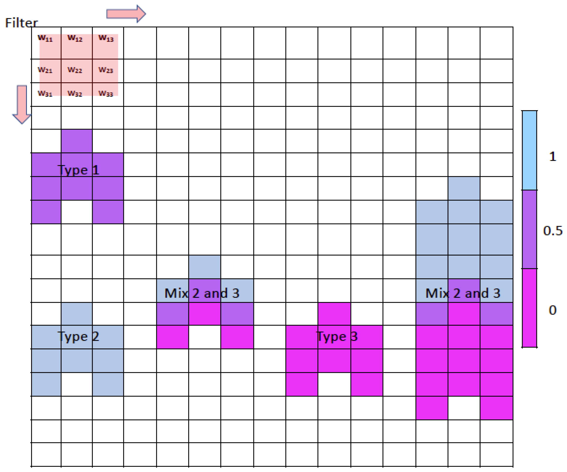
6]. For any sensor, the scope of the spectral information available depends on the instrument’s optical design (e.g., the number of spectral channels, polarization sensitivity, etc.). Spectral differences in scattering behaviors provide clues to layer type. Unlike spectral information, textural information depends on the instrument’s spatial resolution and signal-to-noise ratio (SNR). Additional classification clues can be gleaned from the differing spatial structures exhibited by the scattering from different feature types. An example illustrating the importance of texture information is given below in
Figure 1, which shows the schematic of a 2D image consisting of an array of pixels. A set of filters measuring 3 × 3 (weights: w
i,j; biases: b
i,j) move across the image. Depending on the type of filter applied, convolutions of the filter with the image pixels can retrieve the mean value of any feature within the 3 × 3 “super pixel” (i.e., w
i,j = 1 and b
i,j = 0), the horizontal (or vertical) gradient of these features (i.e., w
1,j = 1, w
2,j = 0, w
3,j = −1 and b
i,j = 0), or the boundaries of the features within the super pixel (i.e., w
i,j = 1 except w
2,2 = 0 and b
i,j = 0). The fine structural details provided by this texture information can distinguish between different feature types that are classified as the same type according to the layer integrated values used by the COSCAs. For example, the COSCA layers shown in the far right of
Figure 1 comprise multiple feature types. The COSCAs identify these layers as being a single type, based on integrated values calculated over the layer vertical extent. However, when CNN texture information is considered, the vertical transitions between different types can be identified within a single COSCA layer. This texture information, therefore, allows us to better exploit lidar profile measurements for clustering and classification. By simultaneously evaluating multiple information sources, convolutional neural networks can identify complex spatial relationships that convey significantly more information than can be derived from simple statistical measurements such as means, standard deviations, and covariances [
7].
While the COSCAs currently use coarsely resolved spatial and spectral information, these algorithms would undoubtedly benefit from the inclusion of additional signal characterizations already available in the data. Optically thick smoke layers provide a striking example. The differential absorption of smoke particles at 532 and 1064 nm results in a constant increase in the attenuated backscatter intensity ratio (i.e., color ratio) with increasing layer penetration depth [
3]. However, the current generation of COSCAs does not use this intra-layer vertical texture information; instead, the cloud-aerosol discrimination (CAD) algorithm uses the layer mean color ratio, which effectively obscures the characteristic structure of the internal changes within smoke layers. Fortunately, deep machine learning (DML) can help exploit intra-layer vertical texture information, and as this paper will demonstrate, can help improve CALIOP aerosol subtyping.
During the recent rapid evolution of deep machine learning (DML) methods, the 2014 development of fully convolutional neural networks (CNNs) has allowed semantic segmentation algorithms to achieve operational maturity [
8]. Since then, CNNs have been widely applied to different domains, including in the field of satellite remote sensing [
9,
10,
11]. When applied to the sematic segmentation tasks, CNNs can take full advantage of combined spectral and texture information for object recognition and classification. Several different semantic segmentation CNN architectures are available, including fully convolutional networks (FCNs) [
8], U-Net [
12], and SegNet, a deep encoder–decoder architecture for multi-class semantic segmentation developed by the Computer Vision and Robotics Group at Cambridge University, UK [
13,
14]. All of these neural network architectures include entangled encoder and decoder processes. The encoder typically uses some well-known building blocks, such as convolutional layers, down pooling, and rectified linear units (ReLU), to ignore fine textures within a feature while extracting coarser descriptive information. The decoder process semantically projects the discriminative features at a lower resolution (e.g., see
Figure 2). The learning that results from the encoder process is then transferred back onto the pixel space at the original (higher) resolution, with each pixel being assigned to a class membership through the decoder. The decoder also uses some of the same building blocks used in the encoding process. Down pooling is used to increase the field of view (i.e., the number of pixels considered) and at the same time reduce the feature map resolution. This works best for classification, where the end goal is to find the presence of a particular class irrespective of the spatial location of the object. Thus, pooling is introduced after each convolution layer to enable the succeeding block to extract more abstract, class-salient features from the pooled features. The 3-dimensional convolutional layers convolve multiple 2-dimensional filters with the original image to derive different aspects of the neighborhood texture information within super-pixels, which are perceptually more meaningful. The convolutional process captures and retains low-level geometric information.
Because semantic segmentation neural networks incorporate neighborhood texture information, they offer new opportunities for improving atmospheric feature classification using 2-D lidar imagery. In this work, we have created a SegNet-like architecture using the routines provided in the MATLAB computer vision and deep learning toolboxes [
15,
16]. We subsequently used the trained CNN to demonstrate the ability of semantic segmentation to improve the classifications currently being delivered by the COSCAs. This study, thus, provides an initial investigation of feature classification within a 2-D framework that explicitly includes spatial texture information, and investigates the role of spatial texture information in the classification of features present in lidar backscatter signals. In
Section 2, we briefly review the architecture of the MATLAB-SegNet model and describe the CALIPSO aerosol subtyping scheme incorporated in the COSCAs.
Section 3 describes the preparation of data sampling and training.
Section 4 compares test results derived from our trained network with the corresponding COSCA results. In the last section, conclusions and perspectives are given.
4. Test and Validation
Validating the CALIOP aerosol typing results is a challenging task, which to date has been attempted by relatively few researchers [
22,
23,
24,
25,
26,
27,
28]. Previous studies have approached this task by determining how well certain combinations of the CALIOP extrinsic data, together with relevant ancillary information, can be mapped into separate, sometimes different families of aerosol types, defined by other researchers and based on other measurements and class definition criteria. Because the aerosol class definitions, instrument capabilities (e.g., CALIOP vs. AERONET), and spatial and temporal coverages are often quite different, these studies can fail to reach satisfactory, dispositive conclusions. Consequently, in this paper we have chosen not to reproduce previous validation studies by substituting our CNN algorithm for the COSCAs. We focus instead on documenting the improvements made in the spatial coherence and contiguousness seen within individual layers and quantifying the increased spatial resolution at which the current CALIOP aerosol types are identified. Future comparisons to altitude-resolved aerosol typing datasets (e.g., derived from Raman or high spectral resolution lidars) should shed additional light on the performance gains that can be realized by adopting machine learning algorithms for CALIOP aerosol typing.
4.1. Case Studies
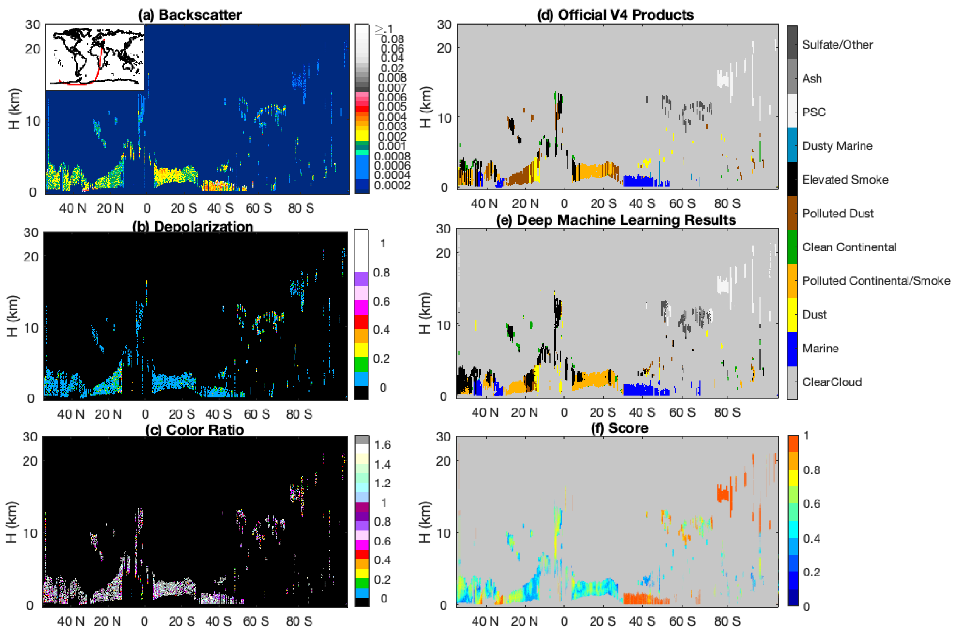
For an initial demonstration of the performance of our trained CNN, we use the nighttime portion of an orbit from 17 August 2010, beginning at 05:56:13 UTC.
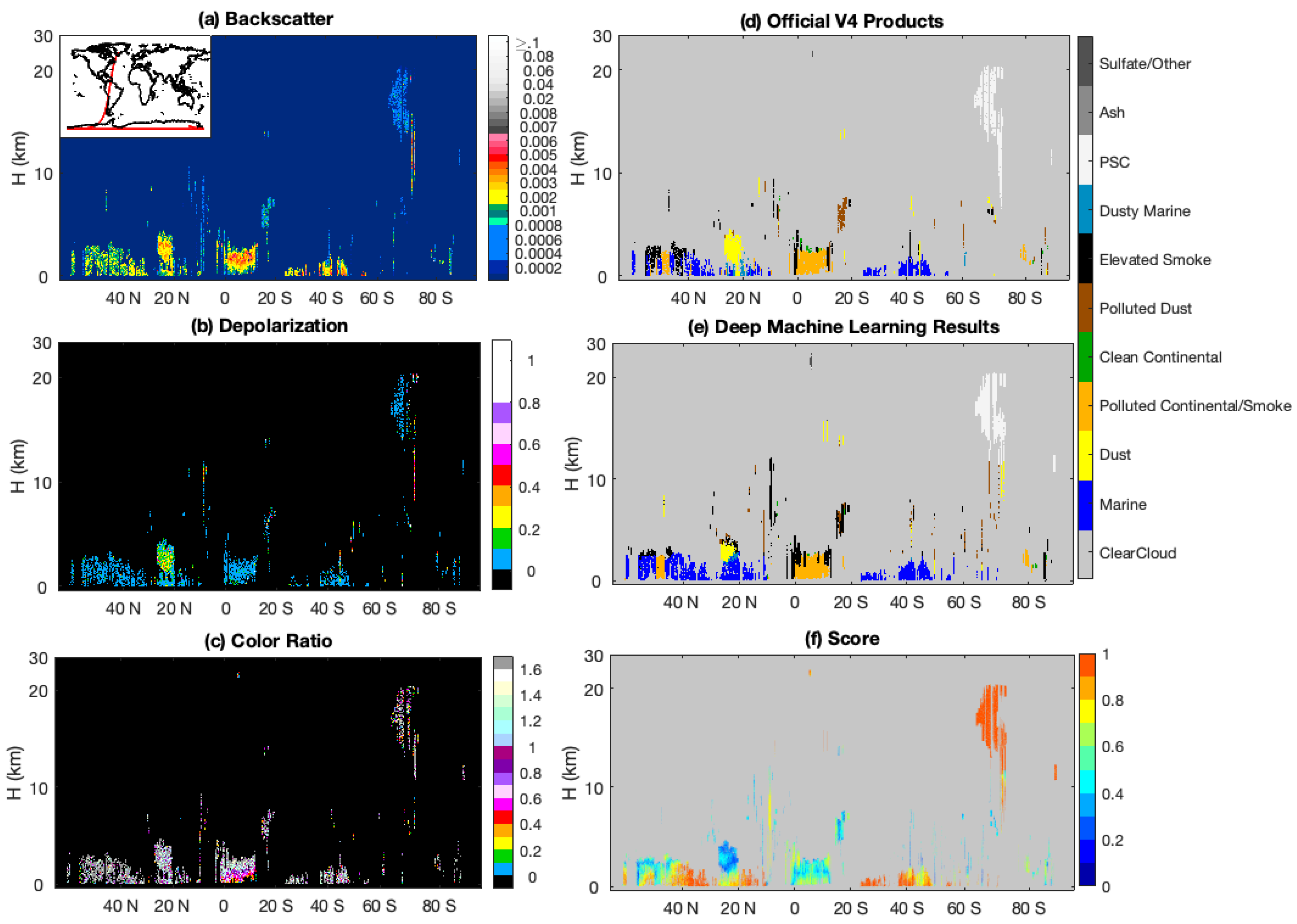
Figure 3a–c shows, respectively, the
β′
532,
δv, and
χ′ measurements that comprise the algorithm inputs.
Figure 3d shows the aerosol subtypes assigned in the CALIOP V4 data products, while
Figure 3e shows the subtypes assigned by our DML method. The results derived by the two methods are seen to be quite similar. The agreement between the V4 data products and the CNN in clouds and clear skies is ~98%, while the agreement within aerosols layers falls to 73%. This disparity in aerosol subtyping is expected. While the V4 COSCAs assign only a single subtype to all pixels within a layer, the CNN is not similarly constrained—the CNN can make multiple subtype assignments within a layer. The added flexibility of the CNN is especially noticeable below ~5 km at ~20° N, where the COSCAs identify a Saharan dust layer transported over the Caribbean Sea that extends from ~4 km to the surface. The CNN classifications in this region show a more physically plausible transition from pure dust in the upper portion of the layer to an intermediate dusty marine mix and finally to a surface-attached marine aerosol in the marine boundary layer. This transitional typing is possible because the textural information encoded in the lower altitudes of the aerosol layer helps sway the subtyping decision. Other obvious differences between the two methods are cross-classifications between polluted continental/smoke and elevated smoke classes and between elevated smoke and polluted dust classes. Both of these are reasonable because these subtypes are frequently found in close proximity to one another and because mixtures of smoke and dust can frequently be misclassified as one of the dominate aerosol class. We also notice that the COSCA products can exhibit abrupt classification discontinuities, where an otherwise unexpected aerosol class is identified within an extended horizontal plume of another class. An example of this behavior occurs around 42° N in
Figure 3, where a column of smoke is embedded in a large area of marine aerosols. While this abrupt change may indicate aerosol mixing, a more likely explanation is intermittent misclassification. In contrast, the CNN’s use of texture information tends to remove these discontinuous classes, thus enabling the CNN to predict a plume of aerosol of the same species (marine) in this same region.
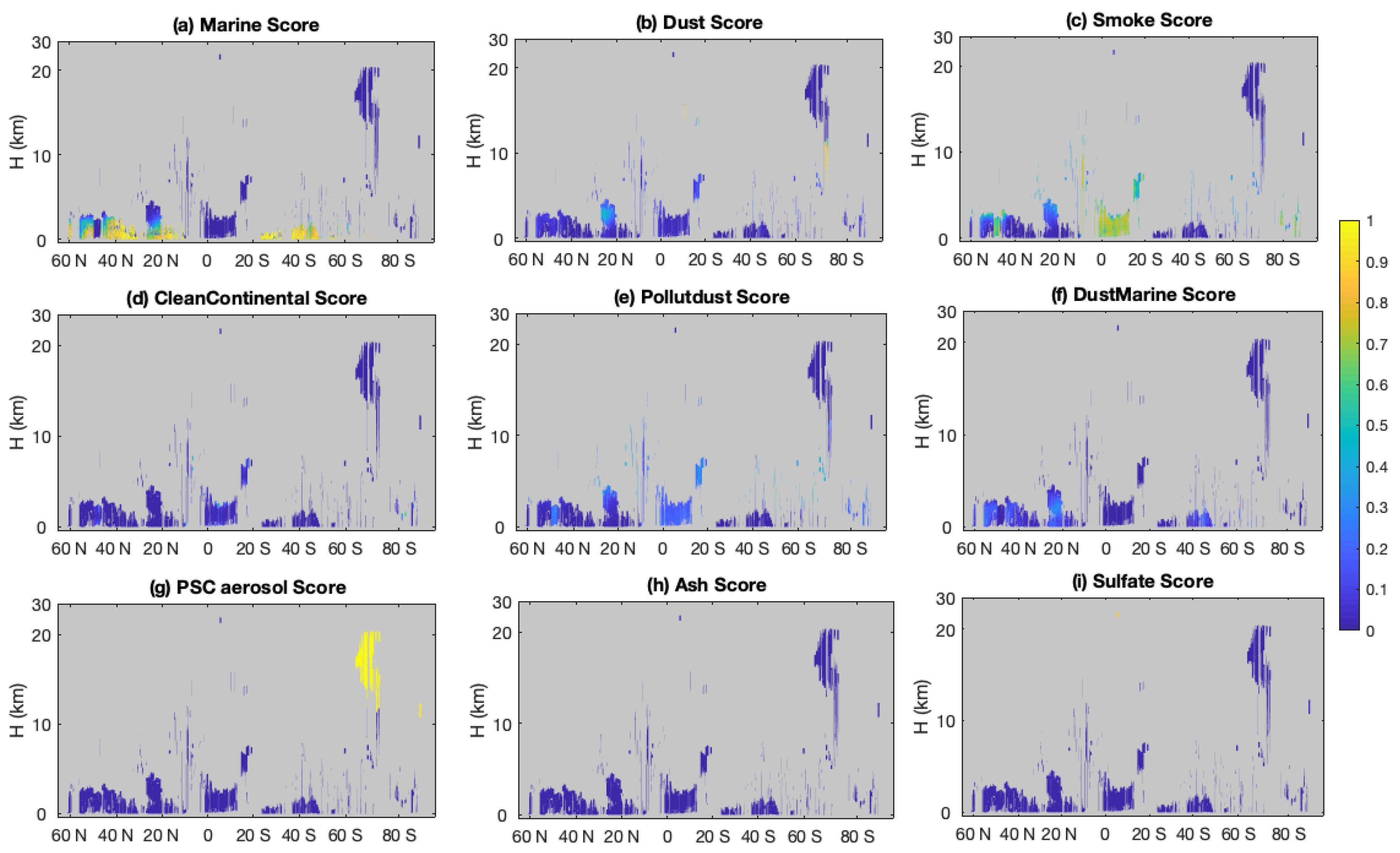
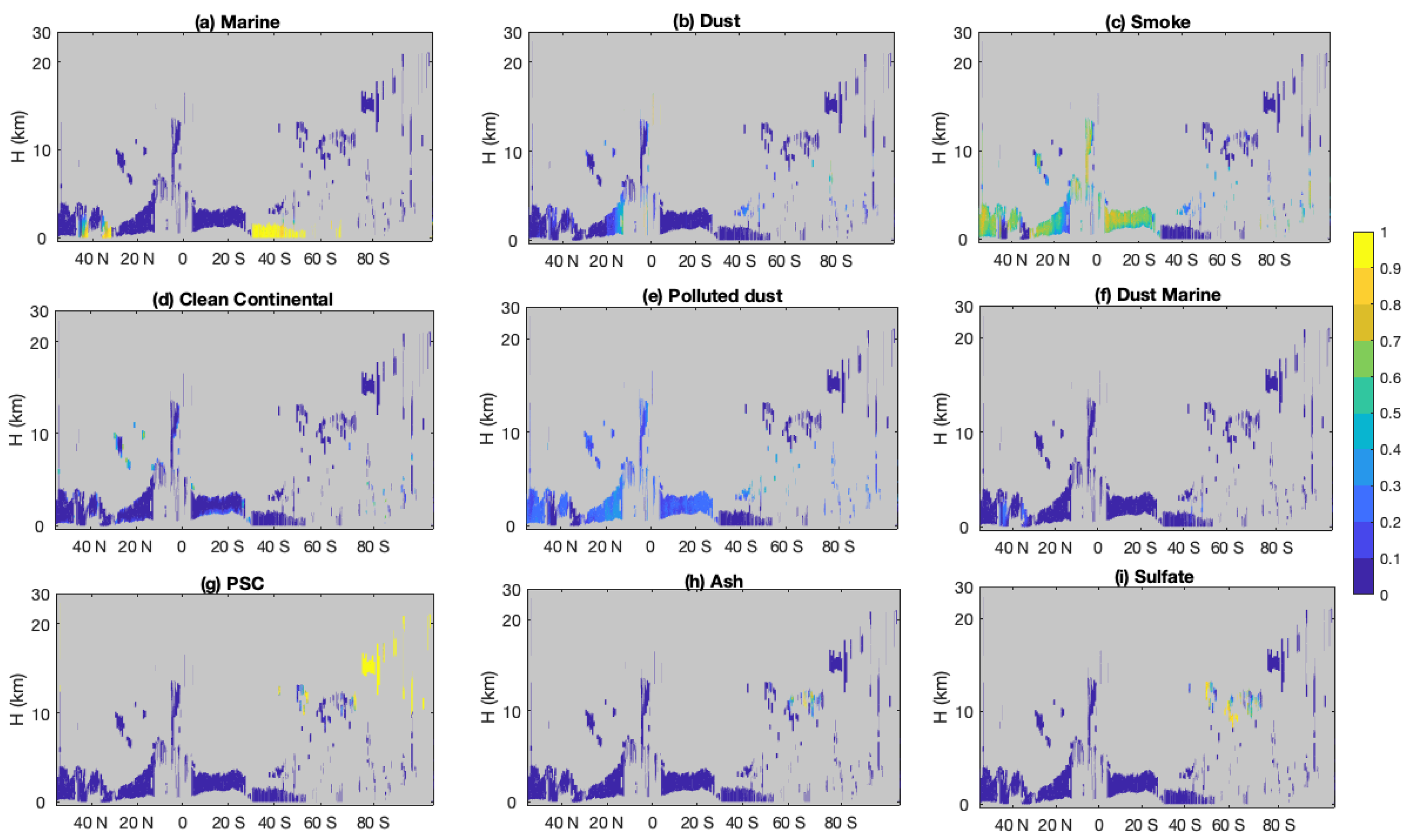
The COSCAs provide only a binary assessment of aerosol classification confidence; any classification is judged as either “confident” or “not confident”. In contrast, the CNN algorithm returns floating point classification scores between 0 and 1 associated with the final categorical label (i.e., the assigned aerosol type; see
Figure 3f), as well as the classification scores (probabilities) associated with belonging to each of the other aerosol subtypes (
Figure 4). As shown in
Figure 3f and
Figure 4a,g, the polar stratospheric aerosols and marine aerosols are identified with high confidence scores, while other aerosol types have low confidence scores, possibly related to mixtures of aerosol types being present or to unintended overlap in the class definitions. The smoke occurring between 10° S to 20° S should be confidently classified based on the increase in color ratio with increasing penetration depth into the layer. However, low confidence scores appear here due to classification confusion between elevated smoke and smoke regimes. If we combine the possibilities of these two regimes, as shown in
Figure 4c, the scores increase, indicating higher confidence that smoke is the correct classification. Low classification scores also appear for dust around 20° N. In the upper part of this plume, dust is confused between smoke and polluted dust (
Figure 4b,c,e), while in the lower part, dust is confused with dusty marine and marine types (
Figure 4a,b,f). According to these scores, the CNN method suggests that there is a possibility of mixing of aerosols away from local sources in the area—Sahara dust could transfer across the Atlantic Ocean, mixing with the smoke transferred from the Amazon basis to the south and marine aerosols lofted from underlying layers.
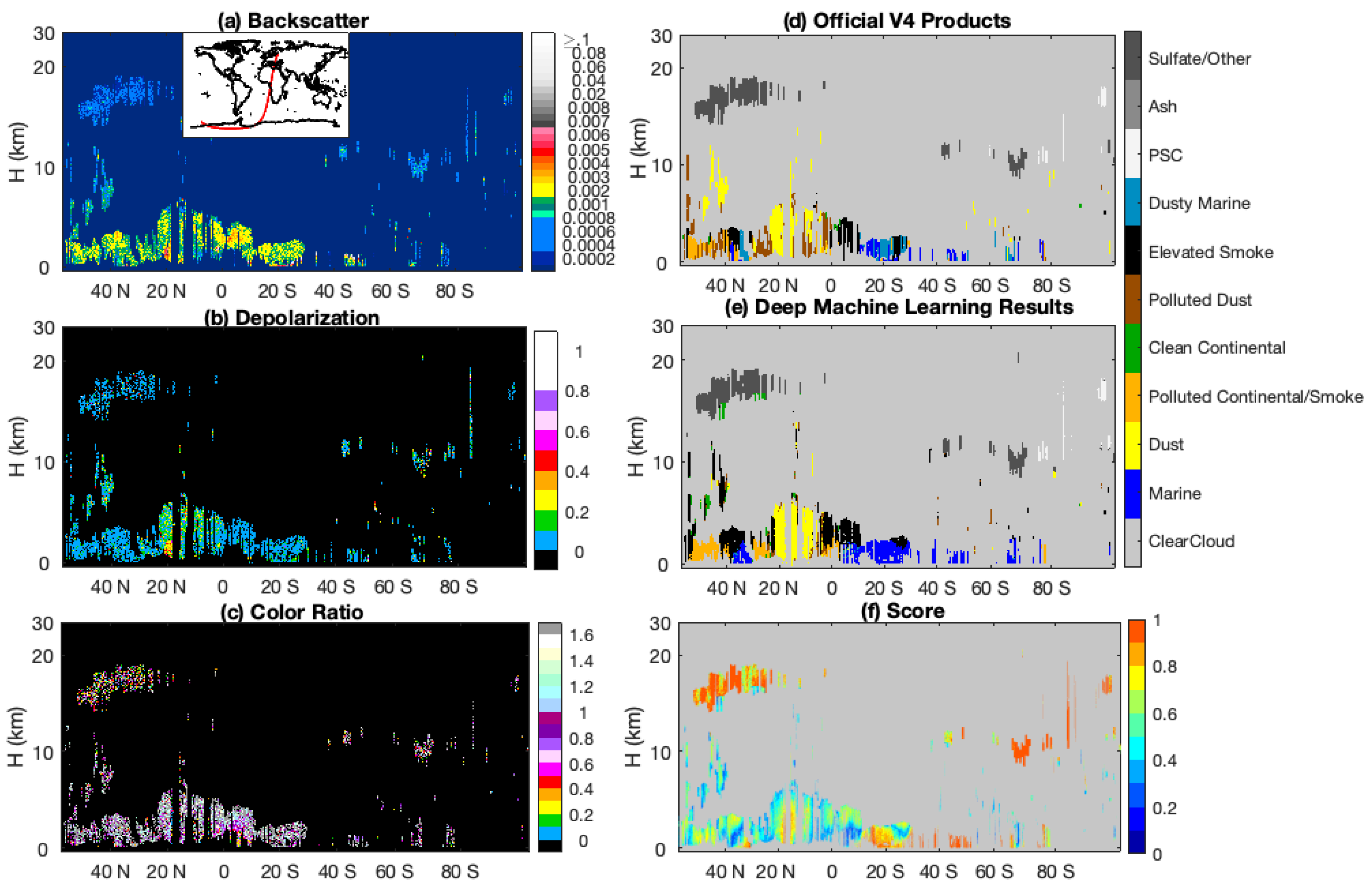
Another case for the nighttime portion of an orbit from 19 June 2011, starting at 23:53:12 UTC, is shown in
Figure 5 and
Figure 6. The agreement between the V4 COSCAs and the CNN in clouds and clear skies is ~96%, while the agreement within aerosols layers falls to 60%—slightly lower percentages compared to
Figure 3. The disagreement is mainly due to different classifications of dust, polluted dust, and polluted continental/smoke class in the troposphere. Between 0 and 20° S, over central Africa where fires frequently occur during this season, the COSCAs and the CNN agree for most of the layers classified as polluted continental/smoke class. There is slight disagreement beyond 20° S near the Namib Desert, where the COSCAs show a mixture of dust and smoke. The CNN classifies these aerosols as smoke, perhaps because the training dataset contains relatively few samples of mixtures of dust and smoke in this region. The fact that smoke can have elevated depolarization ratios also presents challenges for both algorithms in separately identifying dust, smoke, and mixtures of the two.
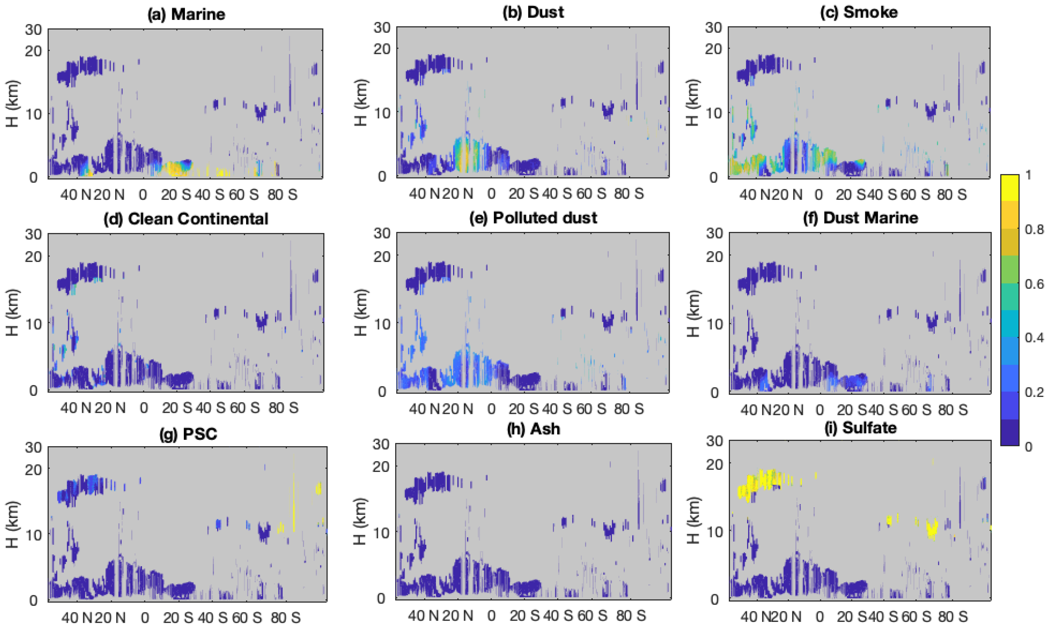
Over the northern hemisphere, smoke is detected beyond 40° N by both algorithms, although the color ratios do not show the typical transition pattern of smoke. Between 20° N and 40° N, the COSCAs classify the plume as a mixture of smoke and dust. The CNN classifies it as polluted continental/smoke class, but assigns low classification scores to the features (
Figure 5f). These low scores (
Figure 6b,c,e) may indicate a possible mixing of smoke and dust. Again, this is a complicated case due to the varying mixture of smoke and dust. The lack of well-defined boundaries separating dust, smoke, and mixtures of the two types, combined with noise in the lidar backscatter signals, can lead the CNN to seemingly erratic and erroneous classifications. Additional in situ measurements in these regions could provide the ground truth information needed to better define the class boundaries for these three subtypes, and hence improve CNN future training.
For marine aerosol, both algorithms agree in the classification. An exception occurs beyond 60° S where the COSCAs classify the features as dusty marine class, while the CNN assigns them marine aerosols. The CNN identifies this region as marine aerosols, most likely due to the use of texture information and less samples of dust marine origin in the training dataset in this region. In the stratosphere, volcanic ash layers from the June 2011 Puyehue-Cordón Caulle eruption [
29] are detected above 10 km from 40° S–70° S. The COSCAs and the CNN agree on the ash classification for much of the plume. They also agree on PSC and sulfate/other classifications over the southern hemisphere.
A third case for the nighttime portion of an orbit from 14 July 2011, starting at 00:42:02 UTC, is shown in
Figure 7 and
Figure 8. The agreement between the V4 COSCAs and the CNN in clouds and clear skies is ~96%, while the agreement within aerosols layers is 81%. The disagreement is mainly due to confusion in classifying dusty marine and marine+smoke mixtures in the troposphere. Around 40° N and 20° S, the aerosols near the ocean seem to be a mix of smoke and marine classes. The COSCAs classify these layers as dusty marine class, while the CNN classifies them as pure marine class. Because we did not define a marine + smoke class in either algorithm, neither method can correctly identify the aerosol type in this case. Again, it is worth noting that accurate identification of arbitrary mixtures of aerosol types remains an exceedingly difficult problem, irrespective of the algorithm(s) applied to the task.
4.2. Statistical Comparisons
Independent characterization of the CNN was conducted using unexamined data from the months of July, August, and September 2010. Aerosol subtypes assigned by our CNN are compared to the assignments reported in the V4 data products in the confusion matrix shown in
Table 1. Each cell reports an occurrence frequency (as a percentage), which maps aerosol subtypes from the CNN (columns) to the COSCAs (rows). These frequencies are normalized so that the sum of each row is 100%. As shown in
Table 1, we again see that the agreement between the two methods in aerosol-free conditions is ~98%, while the overall agreement within aerosol layers is ~62%. For stratospheric aerosols, the two methods agree in ~87% of all cases. In the troposphere, agreements are higher over oceans (~62%) than over land (~57%). This difference is expected. Over land, numerous sources of natural and anthropogenic aerosols are frequently mixed during transport, resulting in stratified layers containing different subtypes. While these subtypes can be correctly identified by the CNN, the COSCAs are constrained to classify each layer as homogeneous. Globally, marine and dust are the most frequently occurring aerosol subtypes [
4], and the agreement between the two methods for these subtypes is reasonably high at ~78% and ~64%, respectively. Relatively good agreement is also seen for clean continental (~67%), polluted continental/smoke (~75%), and all the stratospheric aerosol types.
Subtyping mismatches between the two methods may simply indicate the lack of crisp separation between the CALIOP aerosol classes. Alternatively, mismatches may be highlighting those areas where either the COSCAs or the CNN (or both) have wrongly classified the aerosol. For example, while the agreement for marine aerosols is high (~78%), a substantial portion (~20%) of the COSCA-identified marine aerosols are classified as dusty marine by the CNN. In other words, ~97% of the marine class identified by the V4 COSCAs is classified as marine or dusty marine by the CNN. Similarly, while the agreement for dusty marine class is low (~37%), ~43% of the COSCA dusty marine samples were identified as marine by the CNN and another ~9% as pure dust. Together, these cases account for ~90% of the COSCA-identified dusty marine aerosols. We attribute these subtyping differences to the incorporation of textural information by the CNN algorithm. More importantly, the CNN has the ability to identify multiple subtypes within a single layer.
While the agreement for dust cases is relatively high (~64%), we were initially surprised that it was not a good deal higher, as dust layers are readily identified by their high values of
δp. However, upon reflection, it becomes clear that this less than expected agreement arises from fundamental differences in depolarization ratios used by the two methods. While
δp is an intrinsic aerosol property,
δv is an extrinsic property that depends on the aerosol concentration within a scattering volume. For low concentrations of dust,
δv will be uniformly lower than
δp. Because the COSCAs use layer-integrated properties, they can derive reliable estimates of
δp from
δv using an estimate of the overlying attenuation due to clouds and aerosols [
4]. The disparity in dust classifications arises because unlike the COSCAs, the current CNN architecture does not incorporate an in-line extinction solver that operates on a pixel-by-pixel basis to propagate attenuation corrections into underlying but unclassified pixels or signals. Devising such an intricate companion algorithm is a highly worthy goal. However, it is not immediately clear how it can be accomplished and integrated into the existing CNN framework. (One complication is that adding in-line attenuation corrections will introduce potentially large changes into the texture of the underlying image from one CNN iteration to the next.) This task, thus, lies in the realm of future research that is well beyond the scope of our current investigation.
Approximately 9% of the V4 COSCA dust layers are classified as polluted dust by the CNN and 10% are classified as smoke. This confusion of classifications is likely due to adjacent source locations that may lead mixing of different aerosol types during transport, as explained in
Section 4.3. Because the COSCAs cannot identify mixed types within a single layer, the algorithms are forced to choose between different discrete options. This suboptimal partitioning could bias the characterization of the truth dataset.
For the polluted continental/smoke class, agreement between the V4 COSCAs and the CNN is 74.7%. An additional 9.9% of the COSCA-classified polluted continental/smoke aerosols are classified as elevated smoke by the CNN, bringing the overlap for the two smoke classes to ~85%. However, when classifying layers as elevated smoke, the two methods agree only 54.6% of the time. The agreement for the clean continental subtype is 67%. The poorest agreement is found for the polluted dust class at only 12.4%. This class is defined as a mixture of smoke and dust, with characteristic properties derived from a cluster analysis of AERONET data [
30]. Particularly over Africa, where dust and smoke sources are geographically close, local meteorology can generate arbitrary mixtures of the two types that are not well-represented by the idealized model properties. This lack of specificity in the class definition makes it difficult to identify reliable exemplars for use in the training dataset. Consequently, as seen in
Table 1, the CNN has difficulty distinguishing CALIOP’s polluted dust class from the dust, clean continental, and smoke classes. In addition to the difficulties introduced by an overly broad CALIOP class definition, some fraction of this classification confusion could be due to the CNN’s reliance on
δv rather than
δp as a discriminator for non-spherical particles.
In the stratosphere, 97% of polar stratospheric aerosols are correctly identified by the CNN when compared to the COSCA classifications. While volcanic ash is correctly identified more than 56% of the time, this type is also frequently misclassified as sulfate (28.8%) or high-altitude smoke (8.7%). This is not entirely unexpected, as stratospheric sulfate and ash layers frequently originate from the same sources (i.e., volcanic eruptions), with differences in layer subtyping likely being related to the age of the volcanic plumes. When classifying sulfates, the COSCAs and the CNN agree 78% of the time, with most of the differences being classified as smoke by the CNN. The differences in the sulfate/other subtype could also arise from the COSCA class definition, which defines all stratospheric features for which the 532 nm integrated attenuated backscatter as less than 0.001 sr−1 as sulfate/other. The CNN on the other hand utilizes texture information even when classifying these very weakly stratospheric layers. The overall agreement between the two methods in the stratosphere is ~87%.
4.3. Geographical Comparisons
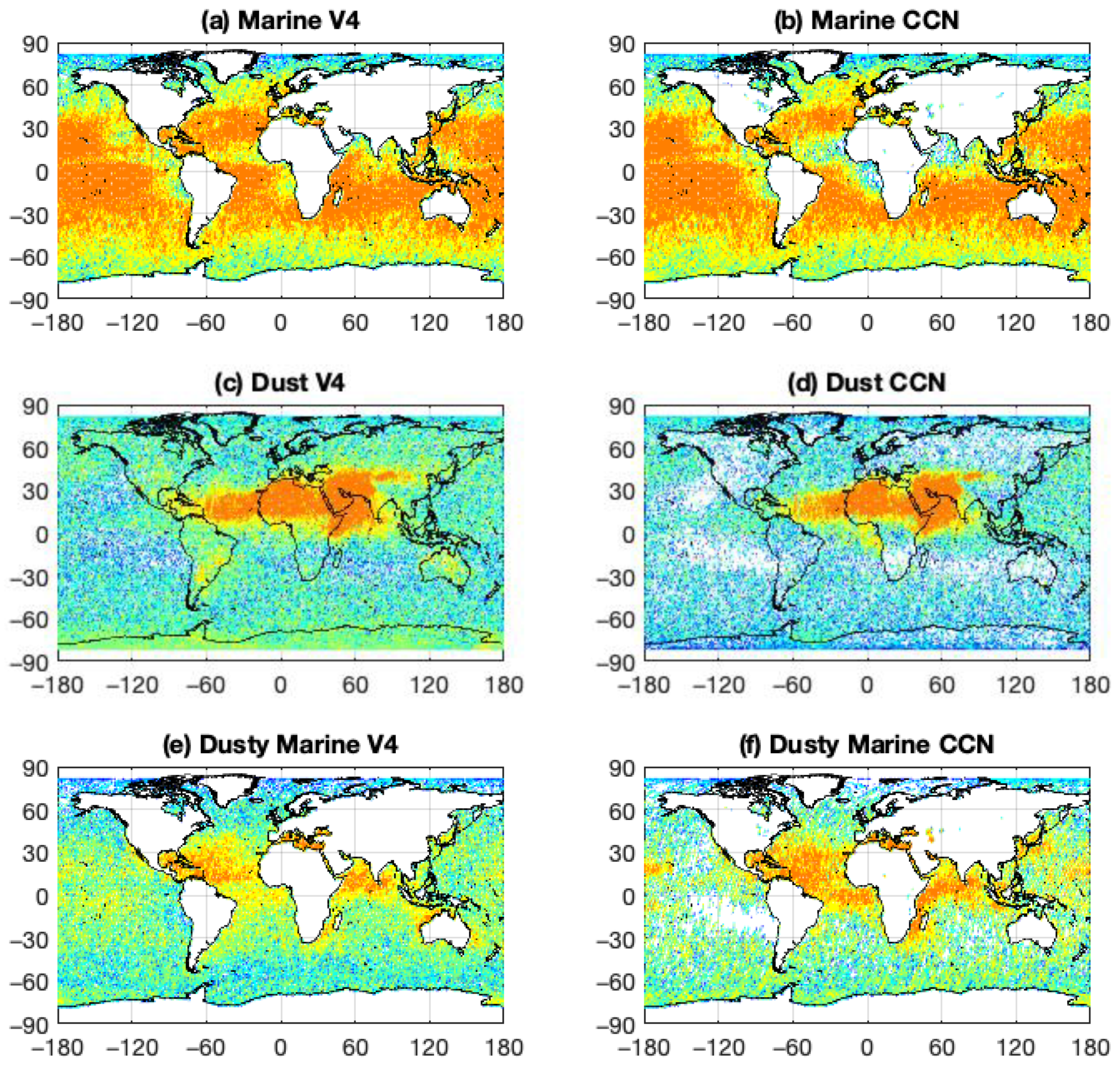
Geographical distributions of aerosol subtypes identified by the V4 COSCAs (left column) and the CNN (right column) for July, August, and September 2010, plus stratospheric volcanic eruption and smoke cases, are compared in
Figure 9. In general, the different tropospheric aerosol types identified by the V4 COSCAs and the CNN are located in similar geographic regions, which are reasonable according to their source locations. As expected, marine aerosols are found in high concentrations over the oceans (
Figure 9a,b). Dust is identified predominantly over the Saharan and Taklamakan Deserts and surrounding areas (
Figure 9c,d), with the CNN results showing relatively lower occurrence frequencies in regions far from natural dust sources (e.g., over the Southern Oceans and Antarctic). Dusty marine aerosols are located over oceans adjacent to various dust sources (e.g., in the Gulf of Mexico, around Africa, over the Mediterranean, etc.; see
Figure 9e,f). While the geographical distribution patterns for dusty marine are generally similar for both methods, the occurrence frequency is typically higher in the CNN results. The higher frequency could come from the bias of ground truth information for dusty marine type in the training dataset, which may also include a small fraction of polluted continental/smoke and marine mixture classes. Polluted dust is pervasive over continental land masses everywhere (
Figure 9g,h) in the COSCA results but is largely confined to African and Asian desert regions in the CNN results. As with the dusty marine class, the geographic distribution patterns identified by the COSCAs and the CNN are similar for the polluted continental/smoke class (
Figure 9i,j), but the CNN occurrence frequencies are substantially higher because the polluted continental/smoke truth information used in the training may contain a mixture of smoke and polluted dust classes. This is especially noticeable in biomass burning regions (e.g., southern Africa and the Amazon regions of South America) and regions with high human population densities (e.g., Europe, East Asia, and the United States). The elevated smoke (
Figure 9k,l) and clean continental classes (
Figure 9m,n) show the same behaviors evidenced by the dusty marine continental pollution/smoke classes; that is, the geographic distributions identified by the two classification algorithms are similar, but in both cases the CNN identifies larger occurrence frequencies. As seen in
Table 1, the more extensive identification of elevated smoke by the CNN frequently comes at the expense of aerosols identified as polluted dust by the COSCAs.
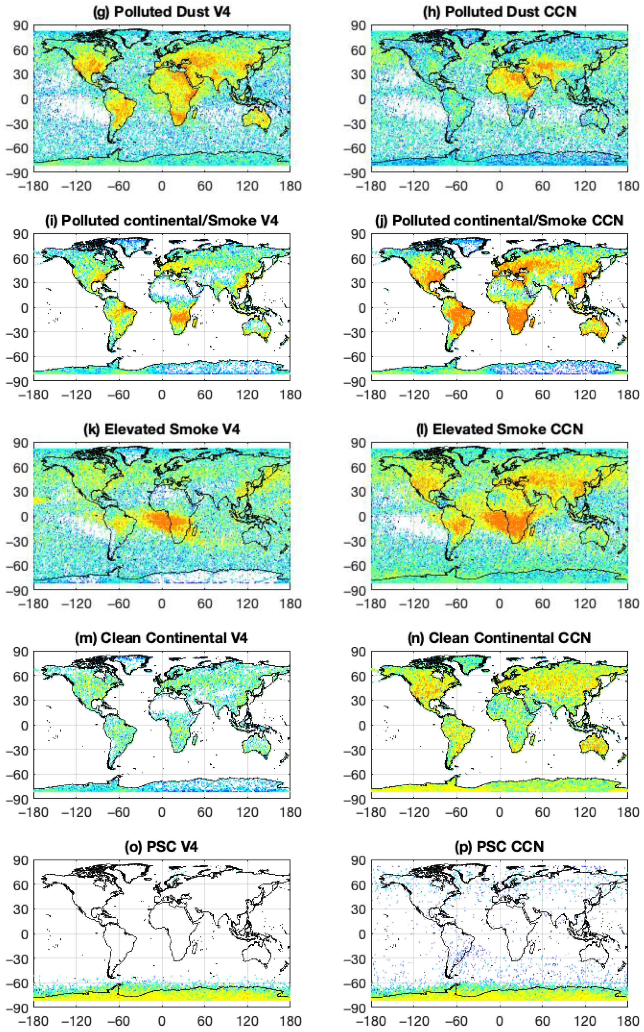
With the exception of polar stratospheric aerosols (
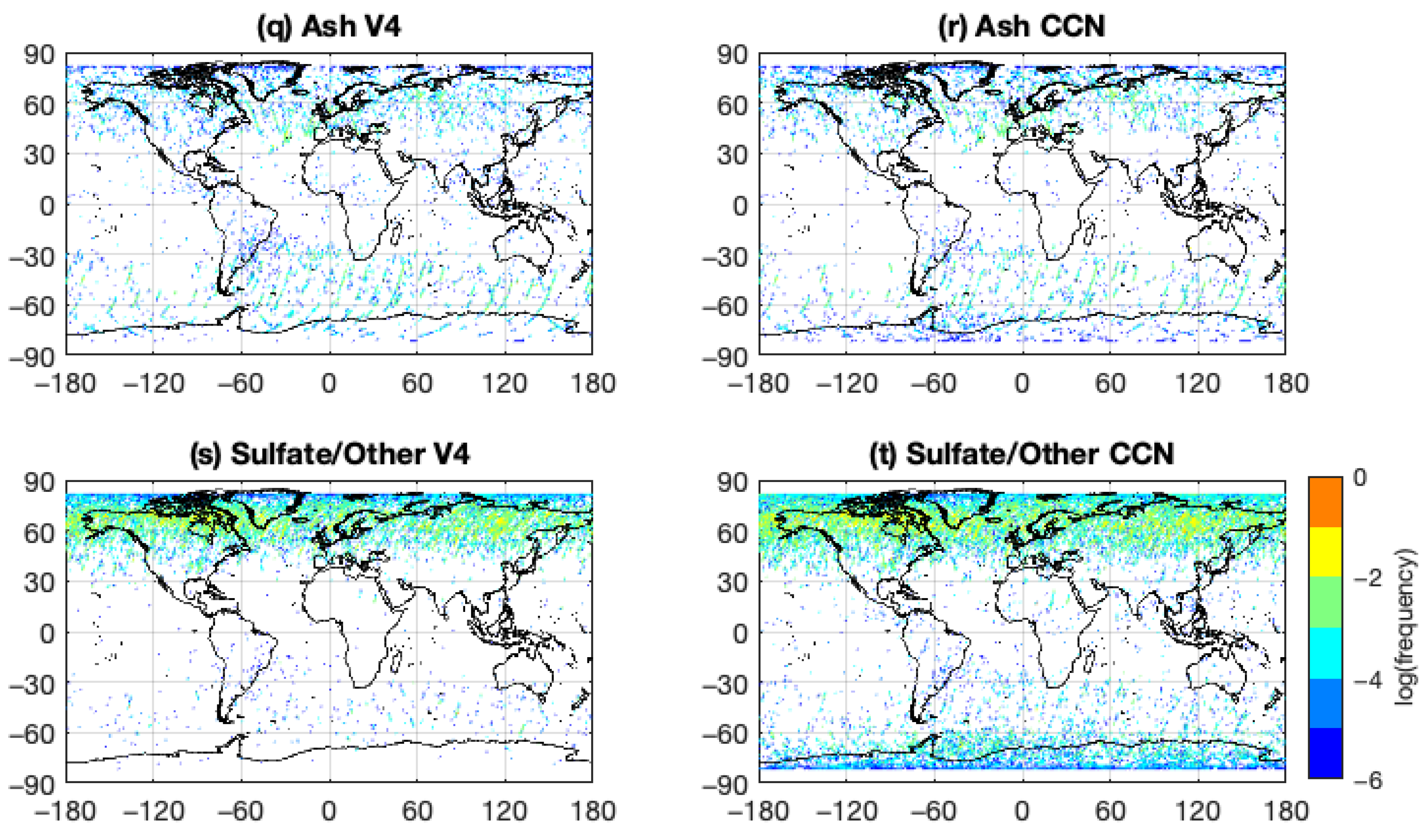
Figure 9o,p), the COSCAs and the CNN largely agree on the spatial distributions and occurrence frequencies for the stratospheric aerosol classes. In the COSCAs, the possible identification of polar stratospheric aerosols is restricted according to season and latitude. Because the CNN is not similarly restricted, it occasionally identifies “polar” aerosols as occurring in the mid-latitudes. Volcanic ash (
Figure 9q,r) is identified only rarely by both classifiers. Sulfates (
Figure 9s,t) are found predominantly in high northern latitudes, consistent with the locations of volcanic eruptions occurring during the study period chosen. The CNN shows a mild propensity for misclassifying some polar stratospheric aerosols as sulfate/other class.
5. Conclusions
Using SegNet, a convolutional neural network (CNN) architecture that implements deep machine learning (DML) methods, we have used the vertical and horizontal texture information intrinsic to space-based lidar observations to classify aerosol subtypes. The CNN method takes advantage of additional independent information that is available in the lidar profiles but not currently being used by the CALIOP operational scene classification algorithms (COSCAs). Our study shows that when using a 1435 orbit training set (i.e., three full months of measurements), the CNN classifier will identify the same aerosol subtypes as the COSCAs in ~62% of the tropospheric cases and ~87% of the stratospheric cases. Given that the CALIOP aerosol class definitions are not discrete, but instead specify mixture continuums (e.g., marine to dusty marine to dust classes) and contain altitude-dependent types (e.g., polluted continental/smoke vs. elevated smoke classes), we find this to be a reasonably good level of agreement. In fact, one might argue that the COSCA classifications, which are taken as truth in this experiment, are sometimes erroneous, simply because the COSCAs are constrained to identify each layer as wholly homogeneous. Because the pixel-by-pixel CNN classifications can identify multiple aerosol subtypes occurring within the predetermined layer boundaries, in these cases the CNN aerosol subtypes may be more accurate. We note, however, that for this iteration of our CNN classifier, we did not attempt to estimate particulate depolarization ratios, but instead used the directly measured volume depolarization ratio, which can cause underestimates in the CNN classifications for dusts and other irregularly shaped, depolarizing aerosol types.
In this paper, we have shown the application of a DML method for aerosol subtype classifications from lidar profile data. The CNN algorithm we have implemented exploits the texture information already embedded in the space-based lidar measurements. Because aerosols can exist in elaborate mixtures of many different types, the goal of this new approach is to deliver a more realistic accounting of the different aerosol types within individual layers. In the future, CNN training sets could be augmented at single-shot resolution with more accurate in situ and remotely sensed field measurements to improve classification skill. These additional training resources should prove particularly beneficial when assessing space-based lidar measurements of aerosol plumes detected in transition zones between major aerosol source regions, where mixing currently poses significant challenges to the methods now being used. A three-dimensional sematic segmentation CNN model with a single profile convolutional kernel that includes geographic and altitudinal information (instead of training over land and ocean and in the stratosphere) should further enhance the classification accuracy.

 ,
, 


