Solar Photovoltaic Forecasting of Power Output Using LSTM Networks


Department of Chemical Engineering, Cyprus University of Technology, Corner of Athinon and Anexartisias, 57, Lemesos 3603, Cyprus
*
Author to whom correspondence should be addressed.
Atmosphere 2021, 12(1), 124; https://0-doi-org.brum.beds.ac.uk/10.3390/atmos12010124
Submission received: 4 January 2021
/
Revised: 7 January 2021
/
Accepted: 13 January 2021
/
Published: 18 January 2021
(This article belongs to the Special Issue Machine Learning for Solar Radiation Estimation)
Abstract
:The penetration of renewable energies has increased during the last decades since it has become an effective solution to the world’s energy challenges. Among all renewable energy sources, photovoltaic (PV) technology is the most immediate way to convert solar radiation into electricity. Nevertheless, PV power output is affected by several factors, such as location, clouds, etc. As PV plants proliferate and represent significant contributors to grid electricity production, it becomes increasingly important to manage their inherent alterability. Therefore, solar PV forecasting is a pivotal factor to support reliable and cost-effective grid operation and control. In this paper, a stacked long short-term memory network, which is a significant component of the deep recurrent neural network, is considered for the prediction of PV power output for 1.5 h ahead. Historical data of PV power output from a PV plant in Nicosia, Cyprus, were used as input to the forecasting model. Once the model was defined and trained, the model performance was assessed qualitative (by graphical tools) and quantitative (by calculating the Root Mean Square Error (RMSE) and by applying the k-fold cross-validation method). The results showed that our model can predict well, since the RMSE gives a value of 0.11368, whereas when applying the k-fold cross-validation, the mean of the resulting RMSE values is 0.09394 with a standard deviation 0.01616.
1. Introduction
In the last century, fossil fuels were the most widely used sources for electrical energy generation, and at present, electrical energy still depends on them significantly. Nevertheless, the constant draw of the fossil fuel reserves, which are already of limited supply, directly affects global climate change (global warming or greenhouse effect) with consequentially various human activities all over the planet [1,2]. According to the World Health Organization (WHO), climate change is one of the greatest health threats of the 21st century [3].
More recently, in 2015, during the United Nations Climate Conference (COP21), 195 countries came together to work on the limitation of global warming. This milestone, also known as the Paris Agreement, stresses the necessity to generate energy through renewable sources so as to provide a better world for the next generation [4]. In this direction, the European Union (EU) is pursuing a set of distinct climate and energy targets. Specifically, the EU has set the goal of the total energy generated from renewable energy sources (RES) to be 30% by 2030 and 100% by 2050.
Among RES, the exploitation of solar energy, along with wind energy, are both the most acceptable and promising. These two sources have the highest chances of getting into the energy market due to their increased potential and availability [1]. Solar energy is the most abundant one since the amount of energy received from the sun is more than the world’s energy consumption requirement. Therefore, solar energy has gathered wide interest and over recent years, remarkable progress has been made in the use of solar technologies for the production of electricity [5].
The utilization of photovoltaic (PV) systems is the most immediate and technologically attractive way to convert solar radiation into electricity [6] and PV systems are mostly preferred due to their numerous advantages; the ability to store the surplus of generated energy in batteries, being environmentally friendly, and having uncomplicated structures and easy applications. Furthermore, the industrial generation of electric power using PV systems requires less labor and machines and has lower carbon emission [6,7]. Hence, the global PV market has experienced enormous growth during the past decade, whereas in some countries, it has emerged to noticeably contribute to the national electricity portfolio as an essential part. In fact, PV solar power represents 7.8% of the annual share in Italy, close to 6.5% in Germany, and more than 1% in 22 other countries [1].
Nevertheless, the power output of the PV power plant exhibits variability at all timescales (from seconds to years) as it is a function of the location, the time, the PV technology used, the cover area of the panels, and their orientation [8,9]. Moreover, power output relies on unpredictable and ungovernable environmental parameters such as solar irradiance, atmospheric temperature, cloud cover, module temperature, wind pressure and direction, and humidity. For instance, PV output escalates in the morning, reaches maximum generation during mid-day, and falls off at dusk due to the sun’s movement. Therefore, the total power generation of a PV dynamically changes in a specified future time period [10,11].
As noted by Rettger et al. [12], even if the terrain is completely flat, as in some plains districts, broken or moving cloud patterns may have a possible impact on the power outputs, whereas in the case of very cloudy sky, the power output may decrease by 10% compared with clear-sky power production. Additionally, changes in ambient temperature can cause differing power outputs from solar panels at any given time, even if the irradiance does not change. More specifically, when the temperature of the solar panel, which is determined by the ambient temperature, the intensity of the sunlight hitting the solar panel, and the amount of cooling of the solar panel by wind, is increased, the output of the solar panels is reduced [12].
The nature of such variables leads to an unstable power generation of a PV system which may lead to control and operation issues for users and administrators of the electricity grid, as a result of sudden surpluses or drops in power output [13]. This intermittent character of the PV power output could create substantial problems in balancing between power production and load demand [14]. Thus, any grid-connected PV system has to be considered as an unpredictable power generator in the utility network, whose production yield variation will adversely affect the power systems’ stability and reliability [15].
Ideally, the independency of PV systems from weather conditions, along with the electrical power supply to the grid based on demand, would be the best option. To achieve that, the power system should be associated with an energy storage, where part of the electricity production will be stored during off-peak hours and will be used when weather conditions are unfavorable. However, this solution leads to a higher construction cost [16].
An alternative solution to this energy loss at power plants and to the dependency on weather conditions is a forecasting scheme of the solar electricity generation from PVs, which would contribute to the reduction of any uncertainties that arise due to the variability of weather conditions. This solution for a more efficient and secure management of electricity grids, leads solar energy trading to a more stable system and also enables a better design of the systems. Therefore, the ability to forecast accurately the energy produced by PV systems is of great importance, especially for power systems in which solar power represents a significant share of the electricity generation mix [17,18,19].
In our work, we aim to establish the optimal management and flexibility of the electricity grid, enabling thus the development of flexible green-powered electricity grids across cities. This can be achieved through the development of a dynamic flow map of the power output of the PVs, not only over the PVs under investigation but over whole regions. More specifically, all PVs will connect on a grid, since a dense network of PVs providing continuous data will enable very high temporal and spatial resolution of forecasts. The database inputs will derive from real-time electricity data of the dense multipoint network of grid-connected PVs. All input data will be stored in the database for current and/or future needs. Moreover, the input data will be processed to extract the normalized power output of each PV, without the need for other equipment, the technical characteristics of the PV or other energy or meteorological related equipment/models for a given area. Additionally, the future PV electricity production will be computed using PV power output prediction models. The database will provide information regarding solar electricity generation from the PVs, failures, daily and annual yield, and statistical analysis of the data. Therefore, the database could be utilized as a service to large scale or aggregated PV managers to provide the system operators for capacity management and scheduling. Figure 1 shows the conceptual framework of the idea behind our work.
As a first step to this objective, in this paper, we demonstrate the necessity to design an intelligent and adaptive prediction model for solar PV power forecasting. In particular, the present paper focuses on developing an accurate model to predict the PV power output for 1.5 h ahead. According to Stylianou et al. [20], PV power output data can provide interesting meteorological information and, more specifically, cloud cover over an area can be estimated in real time. Motivated by this, the model in this work is depended only on historical power output time-series using data from a PV plant in Nicosia, Cyprus. There is no need for any exogenous inputs from sophisticated and expensive data sources such as sky or/and satellite images since the exogenous data may not be always available, expensive to obtain, or unreliable. For instance, weather information may be unavailable to the location where PVs are installed, sky images require special equipment to be processed and recorder and frequent maintenance, and the sensors may be damaged.
The rest of the paper is structured as follows: Section 2 makes a brief review of the importance of PV power generation forecasting and also discusses the classification of forecasting techniques based on input data and time-scale horizon. The preprocessing steps of the input data as well as the forecasting method used are elaborated in Section 3. In Section 4, results are discussed in detail and Section 5 concludes the work.
2. PV Power Generation Forecasting
The technical progress and the fast decline in PV module prices have helped solar energy trading to grow rapidly nowadays. Therefore, solar power forecasting is an important element of energy balancing, especially in countries where the grid is connected to multiple power sources. A reliable PV power output forecasting is a crucial aspect to guarantee grid stability and to enable optimum planning and modeling of solar PV plants. In addition to this, accurate forecasting can provide significant information about how to design an optimal solar PV plant as well as managing the power of demand and supply [4,14].
Furthermore, PV power forecasting is decisive for system and grid operators and managers, as well as for all customers of the grid, since a proper PV power output can provide them with a plethora of benefits. A reliable forecast can assist grid operators to foresee a case of shortage or plentifulness of solar power and can help them to make alternate arrangements for trustworthy dispatching plans. Moreover, it helps with the monitoring of the system, as it can detect anomalies and faults. Accurate solar forecasting also contributes to choosing the most appropriate timing for off-grid maintenance and eliminates the number of units in hot standby. Consequently, the operation cost and the uncertainties on the grid are diminishing. Following this, solar forecasting enhances the stability of the system and increases the penetration level of the PV system [13,14].
In this background, a lot of research has been devoted to the development of appropriate forecasting PV power generation models with the main purpose to achieve higher accuracy and minimum complexity and computational cost [1,4]. Haque et al. [21] proposed a novel hybrid intelligent algorithm for short-term forecasting of PV generated power. Wang et al. [22] suggested a partial functional linear regression model (PFLRM) for forecasting the daily power output of PV systems. Additionally, a one-day-ahead PV power output forecasting model for a single station based upon weather classification, actual historical power output data, and the principle of support vector machines (SVM) was presented by Shi et al. [23]. Li et al. [24] suggested a generalized model, the AutoRegressive Moving Average with eXogenous inputs (ARMAX) model, to forecast the one-day-ahead power output of PV systems for better planning and trading in the electricity market.
Therefore, several techniques have been proposed and developed for an accurate forecasting PV power output method by numerous researchers. Nevertheless, no well-defined criteria exist for each classification as no one method is classified as the “best” in every situation, given the wide range of forecasting problems that exists and each one needs different handling [25]. Generally, the forecasting tools fall into two main categories, indirect and direct approaches.
The indirect approach includes a two-step procedure for forecasting PV power output. The solar irradiance on different time scales based on various approaches is firstly predicted. In the second step of the indirect approach, the forecasted solar irradiance and other associated data such as atmospheric temperature, humidity, wind speed, etc. are often used as inputs to the PV performance model of the plant and thus, the PV power production is forecasted. In the direct forecasting model (second approach), PV power generation is forecasted directly based on some prior information such as PV power output or readily accessed data [22].
Kudo et al. [26] developed both indirect and direct methods in order to forecast the next-day power generation in a PV system. According to their results, the direct method was found to be better, achieving a mean error of 25.6% compared with 28.1% for the indirect method. This information, along with the nature of the data we are provided with (historical data on PV power output) are part of our motivation for adopting the direct forecasting approach in this work.
Besides this classification of indirect and direct approaches, the prediction methods of the PV power generation have been further categorized. Currently, a plethora of solar PV power forecasting techniques exist that are segregated into four main categories named persistence method, physical approach, time-series forecasting methods, and hybrid systems [27].
The persistence forecast model is a fundamental forecasting tool that is commonly used to consider the performance of other prediction models as a reference model. Due to its simplicity, this method may lead to errors in some cases. The physical model comprises a set of detailed mathematical equations, which represent the physical state and dynamic motion of the atmosphere and also use knowledge about the technical characteristics of the power plant. The forecast accuracy of this model is mainly affected by the abrupt changes in meteorological variables [27,28].
One of the oldest known predictive techniques is the time-series forecasting which has deep statistical foundations. Time-series forecasting is a data-driven approach that does not need any internal information from the system. Instead, it is based on past observations, each one recorder at constant successive time intervals. A further distinction of the time-series forecasting method can be made into four broad categories: decomposition approach, smoothing techniques, regression methods, and machine learning based techniques [29].
The combination of two or more approaches, which is known as a hybrid model, can be used in order to ensure the maximum prediction accuracy. These models take advantage of each technique and thus, hybrid approaches show better results than the stand-alone technique for forecasting problems [27]. Nevertheless, the utilization of two or more techniques leads to an increase in computational complexity. Additionally, the selection of a single technique that may perform poorly can influence the accuracy of the hybrid model [1].
Among all forecasting methods, machine learning techniques have drawn attention and are becoming more and more popular nowadays. Machine learning can be used in various domains such as pattern recognition, classification problems, spam filtering, data mining, as well as forecasting problems. The advantage of this method is that the model can find connections among inputs and outputs and also, it can figure out problems that are impossible to be represented by explicit algorithms [30,31].
Thus, many such forecasting models have been developed with high accuracy. One of the most effective techniques is ANN, which is used extensively in the prediction of PV power production. More specifically, ANN is an appropriate method in the case where a non-linearity or/and complicated bonding exists among the data [1]. Moreover, Deep Neural Networks (DNN), which are classes of neural networks with many hidden layers, have made their appearance in the machine learning community with prodigious success during the past years [28].
Most of the researchers [1,27,32] further classify the PV power forecasting techniques based on the origin of the input data and the length of the forecasting horizon to fulfill the requirements of the decision-making process. A brief review of PV power generation forecasting classifications based on input parameters and time horizon is presented in the following subsections.
2.1. Forecast Model Inputs
Forecast inputs have an essential role in enhancing the prediction accuracy and model performance in terms of computational complexity and cost. Therefore, an unsuitable selection of forecast model inputs entails an increase in the prediction error of forecast [27]. Some of the models only require one input, whereas others require more inputs. Nevertheless, the choice of a model is depended on the availability and quality of input data, which is the main limiting factor. To this extend, two main approaches can be found according to the origin of inputs for forecasts: models that use endogenous data and models that use exogenous data.
In the first approach, models use endogenous data that is current and/or past time-series of records of the power production of a PV plant. In the second approach, models use exogenous data, which may derived from local measurements (solar irradiance and weather variables such as temperature, cloud cover, relative humidity, wind speed and direction etc.), information from total sky imagers, satellite images, Numerical Weather Predictions (NWP) (i.e., predictions of temperature, relative humidity, solar irradiance, cloud cover, wind speed and direction, pressure etc.), values from other meteorological databases, and/or information from nearby PV plants.
Based on the above, models using endogenous data benefit from the simplicity in data collection since no other data is necessary. It is worth noting that some studies fall into both groups since some are comparative studies that examine inputs from a different set [4].
2.2. Forecast Horizon
PV power forecasting models can also be categorized based on the forecast horizons. Diverse time horizons are important to make predictions for different aspects of grid operation, such as maintenance of grid stability, scheduling of spinning reserves, or unit commitment [4]. However, there are no specified criteria to classify the forecasting based οn the forecast horizon. Most of the researchers have divided forecasting into three categories [33] based on time horizon, whereas some of them divided it into four categories [14]. Broadly, forecasting can be separated into four major categories as presented below [1,27,33]:
- I.
- Long-term forecast (1 year to 10 years ahead): used for long-term power system planning, since this forecasting category can help with the planning of the energy production, transmission, and distribution organization, according to the future energy demand.
- I.
- II. Medium-term forecast (1 month to 1 year ahead): used for the efficient operation and maintenance of the power system by forecasting the future availability of the electric power.
- I.
- III. Short-term forecast (1 h or several hours ahead to 1 day or 1 week ahead): has a crucial part in optimum unit commitment, control of spinning reserve, evaluation of sales/purchase contracts among several companies. Therefore, short-term forecasting enhances the security of grid operation and is helpful in designing a PV integrated energy management system.
- I.
- IV. Very short-term forecast (1 min to several minutes ahead): also denoted as intra-hour or nowcasting, is used for power smoothing, real-time electricity dispatch, and optimal reserves to assure grid quality and stability.
Nevertheless, several studies indicate that none of the existed PV forecasting models have the same accuracy in terms of the horizon used. Pedro and Coimbra [9], have applied several forecasting models for 1 and 2 h ahead averaged power output. The best performing method was the ANNs optimized by GA (GAs/ANN), where the nRMSE (Normalized Root Mean Square Error) was 13.07% for 1 h and 18.71% for 2 h ahead. Moreover, Lipperheide et al. [32], analyzed the performance of the PV output forecast model over different forecast horizon time. The proposed forecast model produce prediction error (rRMSE) in the range of 3.2–15.5% for forecast horizon from 20, 40, 60 ... up to 120 s. Therefore, it can be observed that the prediction accuracy of a PV power output forecast model diversifies by alternating the forecast horizon even with identical forecast model parameters.
3. Methodology
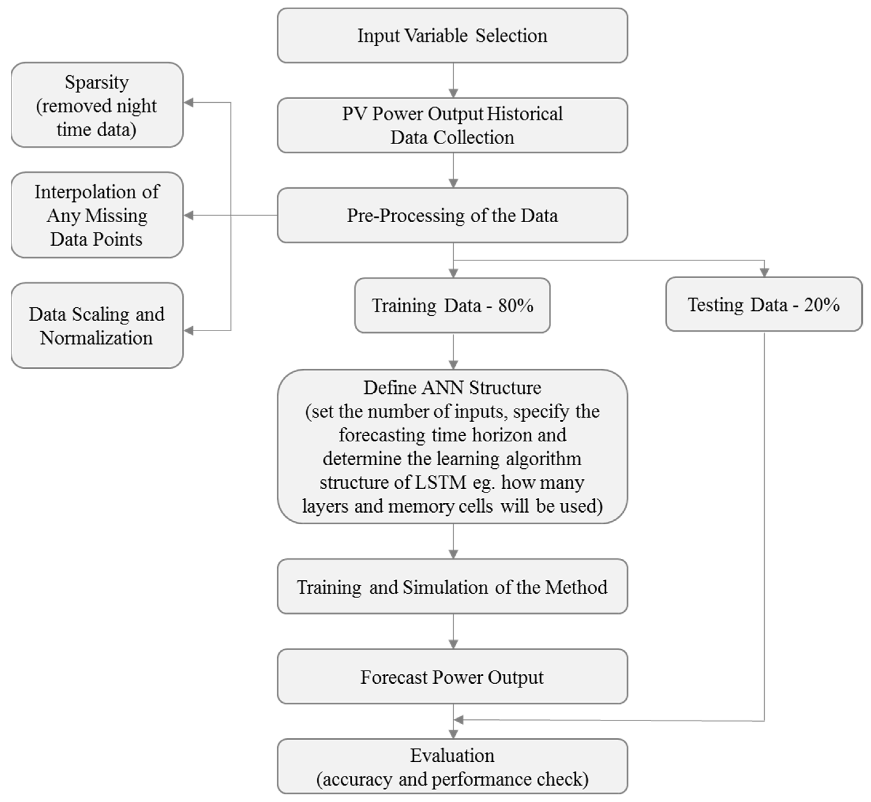
The proposed forecasting method is presented in Figure 2. Firstly, the dataset of PV power output was collected from the database. Then, a data pre-processing, which aims to confirm the input form of the dataset to the Long Short-Term Memory (LSTM) model, was carried out. The pre-processing corresponds to data sparsity, interpolation of any missing values, and data scaling and normalization. 80% of the time series data were used as inputs for the generation of the PV power prediction model, whereas the rest of the data was used to verify that the model could predict the PV power output. This section gives the details of the dataset used, describes the issues that were tackled with during the pre-processing phase, and also presents the forecasting method applied in this work.
3.1. Data Set
Currently, large amounts of PV power output data are available to the public through various websites or can also be provided by a central authority, e.g., an electric utility upon request [34]. For this study, the data were collected through the Aurora Vision, which is a web-based platform enabling customers to remotely manage their PV plants.
The collected data are observations of solar power output (in Watts) from a PV system located in Nicosia, Cyprus. These data points correspond to the value of solar power output over 15 min and are used to form the time-series. Data covers the period from 1 September 2016 to 31 January 2019 (total 84,768 observations). For this study, additional data regarding solar irradiance and other meteorological variables such as GHI, cloud cover, and wind speed and direction were not considered since the objective is to utilize only endogenous data.
3.2. Data Pre-Processing
Any spikes and non-stationary components to the input data of the forecasting models mean that the PV power production model is inappropriate trained and this will drive to high prediction error. Such issues always exist since most of the models utilize meteorological data and historical PV power output data as inputs, that are variable and unpredictable due to weather conditions. Therefore, pre-processing of the input data can decline the inappropriate training problem and computational cost, improving the accuracy of the model considerably [1]. In the following subsections, the data preprocessing techniques employed for sparsity, missing values, and feature scaling, as well as the training and testing technique, are presented.
3.2.1. Sparsity
The collected data of PV power output include night-time values, where there is a presence of many zeros to the PV power output. The data sparsity problem occurs since too many zero values lead to a poorly trained model affecting the performance of the model. Therefore, data sparsity in the input data is an important factor that can affect high prediction accuracy.
To avoid this issue, most of the night-time values were removed by excluding the PV power output values of each date for the time period 20:15–05:00, keeping thus only the time series for the time period of 05:15–20:00 (sixty 15-min intervals for each day). This time interval was selected in order to have at least one zero value for any given day including the summer months. Consequently, the full trained dataset included 52,980 observations.
3.2.2. Missing Data
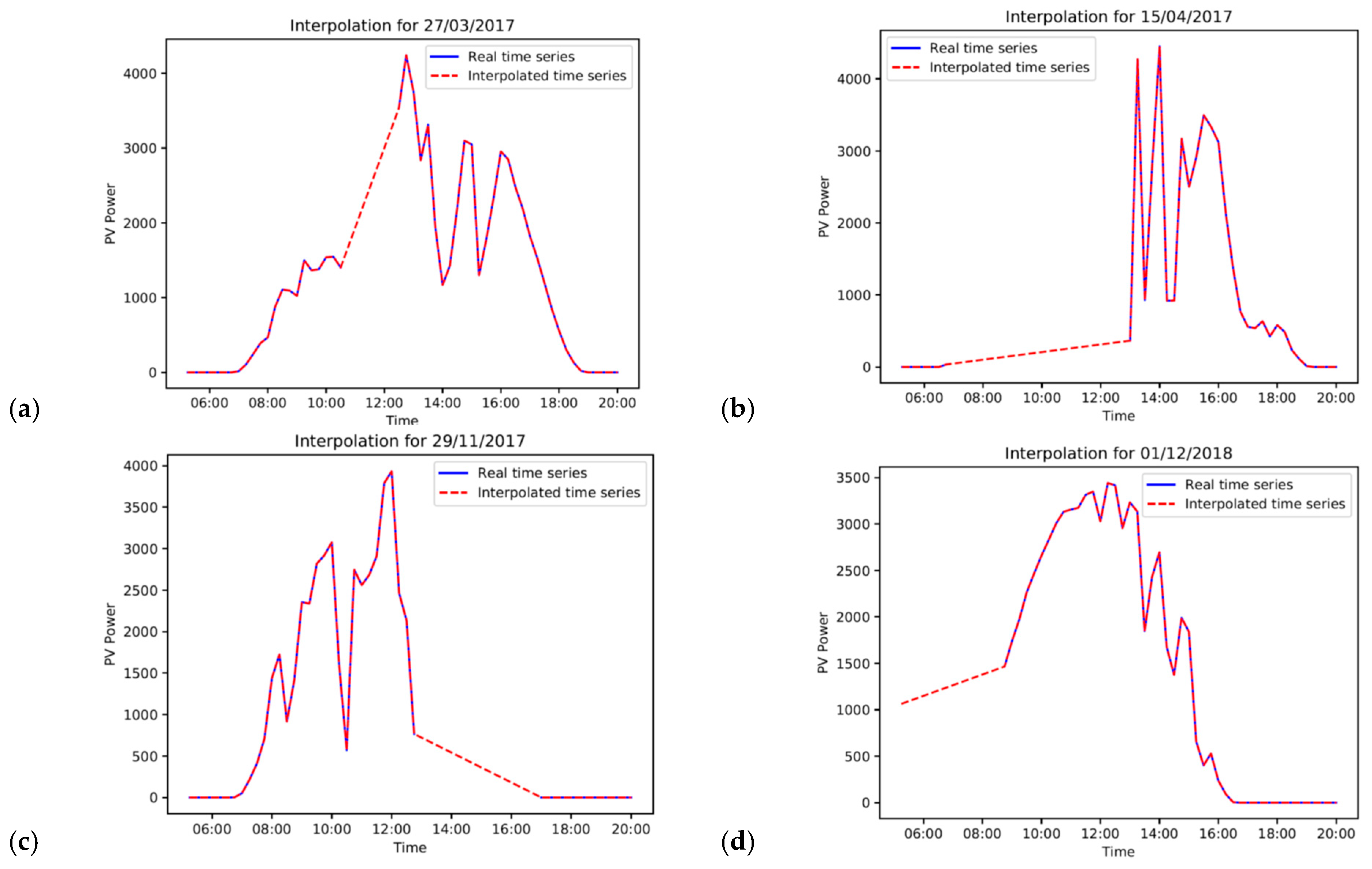
Missing data are usually a result of a failure of the data collection procedure which may be produced by a faulty sensor [35]. Such failures lead to incomplete space time-series and as a result, make precise forecasting difficult. In this work, data examined include a total of 61 observations that are missing on the following dates 27 March 2017, 15 April 2017, 29 November 2017, and 12 January 2018. Missing values represent a small percentage of the total number of observations (61 out of 52,980 observations). However, since our model needs a continuous time-series, we calculate estimates of the missing values of the dataset. The “time” interpolation method was selected as the most appropriate to interpolate the missing values for time-series. Figure 3 depicts the original and interpolated PV power output for the four days on which missing values existed.
3.2.3. Feature Scaling
The dataset used includes variables that are different in scale. Such cases, where different variables might have completely different scales, can lead to a false prioritization in the model of some of the variables. Hence, feature scaling of the dataset is carried out in order to help in accelerating the calculation in the algorithm and also to improve the convergence rates. Once the dataset is trained, it requires less testing time [36].
Normalization, which was applied here, is a common pre-processing method which reduces the dispersion of the collected data. Basically, all the data is rescaled within a particular range from 0 to 1. The dataset was normalized by computing:
where x is the observed value and x’ is the normalized value.
Literature revealed that normalization has a substantial impact on the output of any model since the main objective of data normalization is to ensure the quality of the data before it is fed to any model [37].
3.2.4. Training and Testing Groups
Machine learning has the ability to obtain knowledge on its own, without assuming a specific model relationship, and make accurate predictions. Therefore, in order to evaluate the performance of our model and verify how well our model performs on unseen data, the original time-series was split into two groups: a training and a testing group. The first one was used to train the model, whereas the testing set used to test the model. The testing set is independent of the training dataset but follows the same algorithm as the training group. The error metrics are calculated only on the testing set [38].
In most cases, the split into these two groups would have been random. However, a random subset for time-series would not be representative. Therefore, in this work, the model was trained on a given percentage of the first data and tested on the supplementary of the last data. In particular, the first 80% of the observations (42,384 observations) were used in the training set and the rest of the observations (10,596 observations) in the testing set.
3.3. Model Generation
In this paper, we consider the construction of a Recurrent Neural Network (RNN), which is a class of ANN and is commonly used for time-series analysis. The internal memory state of that network allows the processing of arbitrary sequences of inputs by considering the input from many previous time steps. For that reason, RNN exhibits dynamic temporal behavior. More particularly, RNN behaves like short-term memory since it “remembers” information from previous observations and applies that knowledge moving forward in time [39].
In our study, the number of inputs for the training set was selected to be a vector of 192 timesteps which correspond to 3.2 days of the PV system’s energy production data (a day corresponds to the time period from 05:15 to 20:00: that is, 60 observations per day). The large number of 192 observations can exploit the ability of LSTM cells in order to remember longer-term trends in the data. Therefore, the short-term memory of our RNN model is constituted by 192 timesteps, where each timestep is a 15-min interval. This time interval allows a greater temporal resolution to our model which could be more useful for grid operators than an hourly forecast.
The output values of our model will be the next six power production timesteps into the future since the purpose of our work is to accurately predict the power output for the next 1.5 h. Each input set will slide by 6 observations from the previous set so that the 1st value in the second input set will be the same as the 7th value in the first input set.
In particular, if the first input training set will be X1, X2, ..., X192, the corresponding first output will be X193, X194, ..., X198. Then, the second input training set would be X7, X8, ..., X198, and the second output values will be X199, X200, ..., X204. This gives a total of 7032 sets, each one containing 192 observations. Thus, the outputs do not overlap and are continuous in time.
The training output consists of the real power values, that the RNN will then use to compare with its predictions in order to learn. Therefore, it consists of sets of 6 observations starting from the 193rd observation (since the previous 192 observations used in order to have the first set of predictions). Again, this gives a total of 7032 sets but now each one contains 6 observations.
Among RNNs, Long Short-Term Memory (LSTM) networks have shown the best performance and over the past years, the interest in PV power prediction using LSTM networks is increasing [40]. Lee and Kim [41] have developed two types of ANN methods, a DNN method and two LSTM based methods for the prediction of PV power output using a dataset from a PV operator located in Gumi City in South Korea. The first LSTM model considered four meteorological factors (temperature, humidity, cloudiness, and radiation) and two seasonal factors (month of the year and day of the month), while the second LSTM model (LSTM2) used only the four meteorological factors. Both methods had three hidden layers and an output layer for the hourly PV power output. The results showed that the proposed LSTM model yields the best performance compared to the proposed ANN, ANN2, DNN, LSTM2, and also to the conventional methods Arima and S-Arima.
Abdel-Nasser and Mahmoud [42] have proposed the use of LSTM to accurately forecast the power output for 1 h ahead of PV systems. They used two PV datasets from two different locations in Aswan and Cairo, Egypt. Authors trained and tested 5 LSTM models using different architectures: LSTM network for regression (model 1), LSTM for regression using the window technique (model 2), LSTM for regression with time steps (model 3), LSTM with memory between batches (model 4), and stacked LSTM with memory between batches (model 5). All the models used purely endogenous, historical PV data as input. The proposed model 3 significantly outperformed the other models, and thus was then compared with three forecasting models: multiple linear regression (MLR), bagged regression trees (BRT), and neural networks (NN). Again, the proposed method had the lowest error in terms of RMSE for both datasets.
Jung et al. [43] presented a stacked LSTM–RNN model in their work for the prediction of the monthly power output of PV plants at new sites. The proposed method utilized historical data from 164 distributed PV facilities for approximately 5 years. Eight variables including the month of operation, the estimated solar irradiance, the mean monthly temperature, the relative humidity, the wind speed, the precipitation, the cloud amount, and the duration of sunshine as inputs. The predicted values of power output were compared with the actual values of power output of the test plants through cross-validation. The results showed that the proposed method successfully captures the temporal patterns in monthly data and also estimates the potential of power production at any new site.
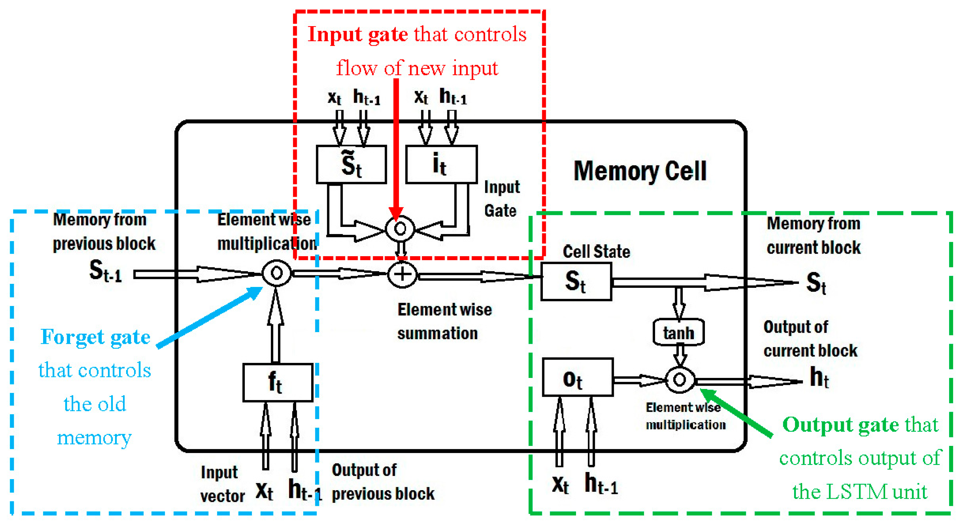
In this work, the LSTM network, which is a significant part of the RNN, was also considered. LSTM neural networks can solve long-term dependency problems. Unlike RNN networks that use temporal information of the input data, LSTM has a special neuron structure called memory cell which can store information over an arbitrary time. A common architecture of LSTM unit is composed of the memory cell which is connected through successive gates. The forget gate sets what information to throw away safely from the memory cell. The input gate decides which values from the input to update the memory state, and finally, the output gate generates the output for the current time-step based on input and the memory cell. A diagram of an LSTM unit can be seen in Figure 4.
An extension of the LSTM model is the stacked LSTM model which has multiple stacking hidden layers, and thus, it has the advantage of enabling the model to acquire information about the raw temporal signal at each time step. Additionally, the stacked LSTM model can expedite convergence and improve the non-linear procedures of raw data since the parameters of such models are spread throughout the space [28,42,44].
Figure 4.
Diagram of a Long Short-Term Memory (LSTM) unit [45].
Figure 4.
Diagram of a Long Short-Term Memory (LSTM) unit [45].

Therefore, we built a stacked LSTM with multiple hidden layers where each layer contains multiple memory cells. This stacking of several LSTM layers for a deep LSTM-based neural network is meaningful since many non-linear mapping layers between inputs and outputs are utilized for hierarchically feature learning. Each layer processes some part of the task we wish to solve and passes it on to the next until, finally, the last layer provides the output. According to Abdel-Nasser and Mahmoud [42], higher LSTM layers can capture abstract concepts in the sequences, which can improve the PV power forecasting results. Thus, for this work, 4 layers of 50 memory cells/neurons each were used to have a model with high dimensionality that can capture complicated patterns. Furthermore, dropout regularization of value 0.2 was used to avoid overfitting.
4. Results
As mentioned above, the forecasting model was defined and trained, respectively, in order to obtain the best forecasting result. In this section, the collected PV power output data was used to evaluate the performance of our model. Firstly, it was examined whether the model can accurately predict the PV power output values in the test set, which correspond to the period from 8 August 2018 to 31 January 2019. The model was not trained on these test set values and, therefore, they constitute unseen data for our model.
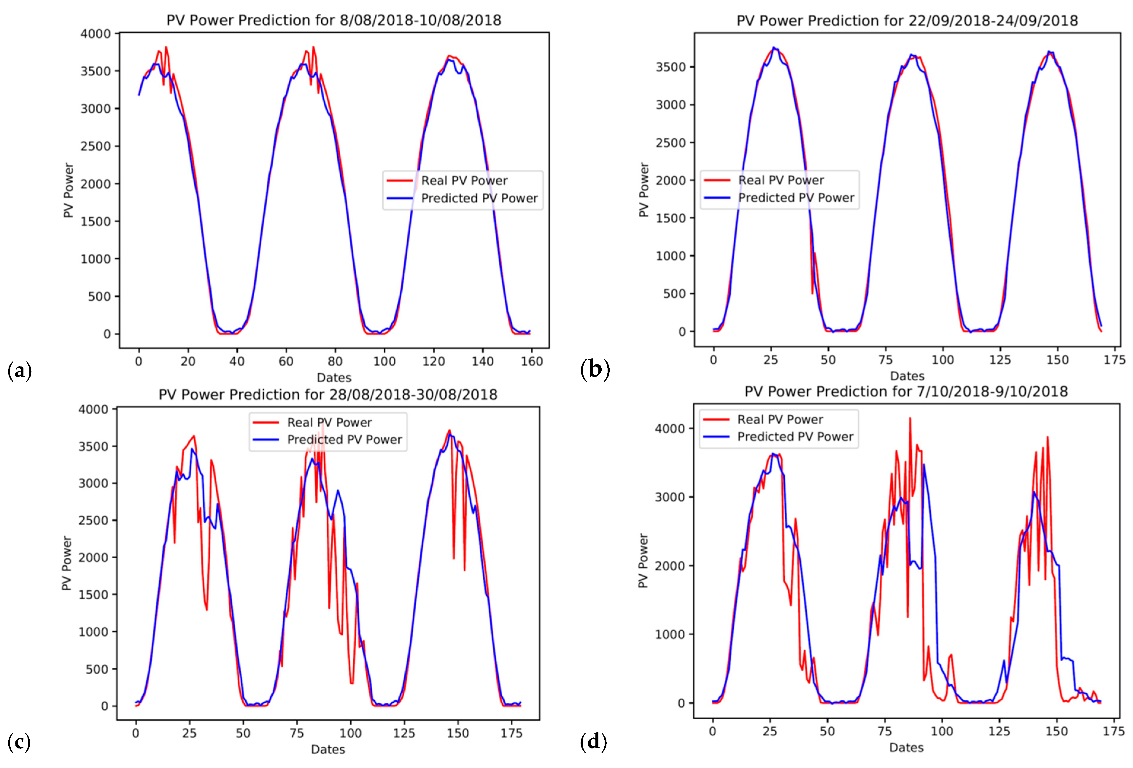
A useful starting point for assessing the model applied is by using graphical tools, which can provide a qualitative assessment. As Tukey said: “There is no excuse for failing to plot and look”. Figure 5 shows the actual (red line) and the predicted (blue line) PV power output time-series for some selected days of the test set. A visual examination of the patterns of power output indicates that our model can predict quite well, especially when the actual PV power output signal is smoother (a & b). It is worth noting that the test set only includes data from the autumn and winter months. Therefore, it is anticipated that our model will behave in a similar or even better manner for most of the days during spring and summer months, since Cyprus has abundant sunshine over these periods.
Moreover, it can be observed from Figure 5c,d that during days with a lot of sharp fluctuations in the actual PV power output, the predicted PV power output is not far off. Most importantly, the predicted power output signal seems to react to each fluctuation and to follow its trend, thus capturing the overall behaviour of the real power output time series.
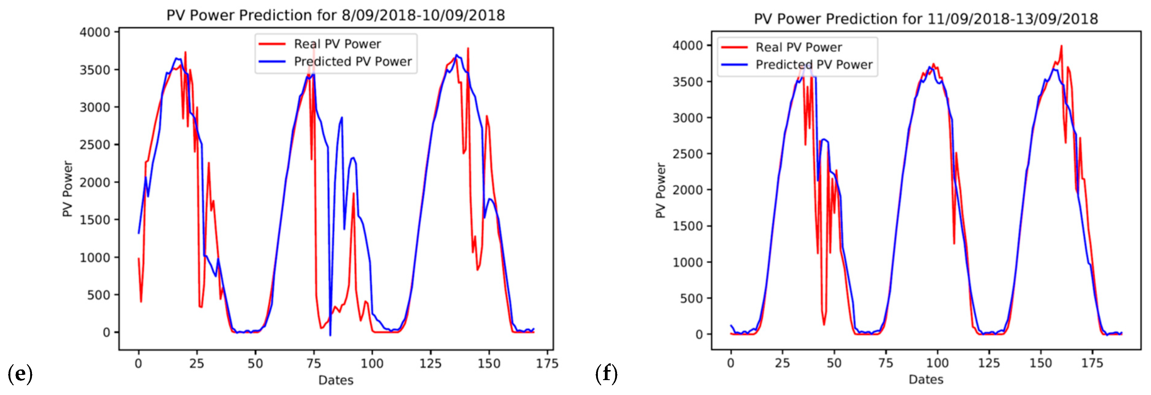
Furthermore, Figure 5e,f further display the variational patterns of the actual and predicted PV power output of six consecutive days from 8 September 2018 to 13 September 2018. As can be seen, the actual PV power output signal has erratic fluctuations with sudden decreases. However, there are some time periods during the same days where the power output time-series signal is smooth. These two graphs indicate that the actual power output of at least the previous day affects the trend of the predicted power for any given day. Nevertheless, our model can still make good predictions moving forward from a day with a fluctuating power output to a smoother one and vice versa.
Although the graphical examination is essential, it does not permit quantitative assessment. Therefore, to further validate our model a prediction performance metric applied to the testing data set in terms of Root Mean Square Error (RMSE). This is calculated as the square root of the mean of the squared differences between the predictions of our model and the real PV power values of the test set. Then, the RMSE value was divided by the range of the PV power values in the test set to get a relative error as opposed to an absolute error. This gives a value of 0.11368 which indicates a good prediction accuracy for our model.
Nevertheless, a different value of the performance metric can be calculated every time we run our model and evaluate its performance on new data. Therefore, judging our model’s performance only on one test gives us a single test metric and does not give the best indication of how the model will perform over a wide variety of test data. For that reason, k-fold cross-validation addresses this problem. In this technique, the original sample is divided randomly into k sub-samples. These k sub-samples are further divided into two groups for testing and training. In the first group, a single sub-sample is considered as the validation data, whereas the rest of the k sub-samples are classified in the second group. This procedure is repeated k times until each k sub-sample is to be used exactly one time as the validation data. Thus, the results are independent of the set of the training data since using only one data set (with its statistical particularities) can limit the robustness of the conclusions [38,46].
Note that the original test set is held out from this procedure. Cross-validation aims to evaluate the stability of the model performance: that is, how generalisable the model is. Due to this, cross-validation creates multiple models on subsets of the training data and applies them to the remaining data from that subset.
For our problem, we performed 10-fold cross-validation where the training set is split into ten groups. Nine of these groups were used as the training set and the remaining group as the test set. This way, there are 10 combinations of training and test folds and for each one, the RMSE was obtained. The mean of the resulting RMSE values is 0.09394 with a standard deviation 0.01616. Since this value is very close to the one we found to the test set, we can safely conclude that our model is not overfitting. In a different scenario, the difference between the two RMSE values would be large.
As previously stated, LSTM networks are designed to model the dynamics of the data as well as to avoid long-term dependency problems. For that reason, several researchers have proposed various LSTM based models for the prediction of PV power generation, as shown in Table 1. Yongsheng et al. [47] state that RMSE of short-term PV output forecasting should be less than 20%. Although most of the studies presented in the table seem promising regarding the error performance, they utilize meteorological-related variables such as solar intensity, humidity, air temperature, cloudiness, and wind speed and direction as inputs. Such exogenous inputs make the prediction of power output significantly challenging since data/information like these, may be unavailable for the location of PV sites examined.
Nevertheless, the LSTM model proposed in the work of Abdel-Nasser and Mahmoud [42] and our study have a significant difference from the other studies since both attempt to estimate the PV power output using only endogenous data. More specifically, both studies receive time series of PV power production data in order to produce the output. Among these two studies, there exist two main differences. The first one concerns the number of timesteps that are used as inputs and the second is related to the number of cells per layer. Ahmed-Nasser and Mahmoud used 1 or 2 inputs with one-hour timesteps and one or two layers with 4 LSTM cells per layer. On the contrary, our work uses 192 timesteps with 15-min intervals for inputs and 4 layers of 50 memory cells each. The larger number of timesteps is useful for LSTM cells to remember longer-term trends in the data. In addition, our slightly larger network of 4 layers would perform better than the smaller ones as presented in Ahmed-Nasser and Mahmoud’s work.
5. Conclusions
Solar PV energy generation forecasting is one of the most challenging tasks mainly due to the intermittency of weather regimes. Forecasting models of PV power output can be deployed to improve the planning, operation, and stability of those systems as well as to increase their penetration level. Building effective predictors that depend only on historical data requires statistical methods for inferring dependencies among past and short-term values of observed values. This paper discussed the utilization of a deep RNN model to deal with PV forecasting problems. More specifically, a stacked LSTM network was considered in order to forecast the PV power output from a PV station over 1.5 h ahead in time. According to the results, our forecasting model can predict well, since a visual examination of the results indicates that the predicted power output signal reacts to each fluctuation and follows the trend of the actual power output signal. Furthermore, the RMSE of our model when applied to the test data gives a value of 0.11368, whereas when applying the k-fold cross-validation, the mean of the resulting RMSE values is 0.09394 with a standard deviation 0.01616.
Nevertheless, fine-tuning of our predictive model will enhance the accuracy of the forecasts. This consists of finding the best values of the so-called hyperparameters which are the parameters that are fixed during training, and therefore, are not learned by the model. The most basic hyperparameter tuning method is a grid search, which gives a space of possible hyperparameter values. As a first step, a model for each combination of hyperparameter values is constructed, then each model is evaluated via K-Fold cross-validation, and finally, the model which produces the best results in terms of K-Fold cross-validation is selected. Future research includes the tuning of the following hyperparameters: (a) the batch-size, (b) the number of epochs, and c) the optimizer.
Moreover, future work will focus on further improvement in the performance of the given forecasting model. Therefore, the model will be explored in greater detail by utilizing larger datasets and will be tested independently in as many locations as possible. Furthermore, since the forecasting error increases with the increase of the time-scale of the forecast, shorter time horizons such as intra-hour or nowcasting will be applied to our estimation technique. Different RNN architectures of LSTM models will also be utilized in order to compare our forecasting results with the results of other methods.
Author Contributions
For this article, M.K. designed and performed the training and testing of the LSTM model, evaluated the results, and contributed to the writing of the manuscript. S.P. carried out the data collection and contributed to the writing of the manuscript. A.G.C. conceived the original idea of the project and was in charge of the overall direction and planning. All authors have read and agreed to the published version of the manuscript.
Funding
This research received funding under SOLAR-ERA.NET Cofund Joint Call and the Cyprus Research Promotion Foundation (KOINA/SOLAR-ERA.NET/1216/0014).
Institutional Review Board Statement
Not applicable.
Informed Consent Statement
Not applicable.
Data Availability Statement
The data presented in this study are available on request from the corresponding author and the consent of the PV company that provided the data.
Conflicts of Interest
The authors declare no conflict of interest.
References
- Das, U.K.; Tey, K.S.; Seyedmahmoudian, M.; Mekhilef, S.; Idris, M.Y.I.; Van Deventer, W.; Horan, B.; Stojcevski, A. Forecasting of photovoltaic power generation and model optimization: A review. Renew. Sustain. Energy Rev. 2018, 81, 912–928. [Google Scholar] [CrossRef]
- Dincer, I. Energy and Environmental Impacts: Present and Future Perspectives. Energy Sources 1998, 20, 427–453. [Google Scholar] [CrossRef]
- Campbell-Lendrum, D.; Prüss-Ustün, A. Climate change, air pollution and noncommunicable diseases. Bull. World Health Organ. 2019, 97, 160–161. [Google Scholar] [CrossRef] [PubMed]
- Antonanzas, J.; Osorio, N.; Escobar, R.; Urraca, R.; Martinez-De-Pison, F.J.; Antonanzas-Torres, F. Review of photovoltaic power forecasting. Sol. Energy 2016, 136, 78–111. [Google Scholar] [CrossRef]
- Thirugnanasambandam, M.; Iniyan, S.; Goic, R. A review of solar thermal technologies. Renew. Sustain. Energy Rev. 2010, 14, 312–322. [Google Scholar] [CrossRef]
- Goetzberger, A.; Hoffmann, V.U. Photovoltaic Solar Energy Generation; Freiburg Springer: Berlin/Heidelberg, Germany, 2005. [Google Scholar]
- Ayvazoğluyüksel, Ö.; Filik, Ü.B. Estimation methods of global solar radiation, cell temperature and solar power forecasting: A review and case study in Eskişehir. Renew. Sustain. Energy Rev. 2018, 91, 639–653. [Google Scholar] [CrossRef]
- Pelland, S.; Remund, J.; Kleissl, J.; Oozeki, T.; De Brabandere, K. Photovoltaic and Solar Forecasting: State of the Art; IEA PVPS: Paris, France, 2013; Volume 14. [Google Scholar]
- Pedro, H.T.C.; Coimbra, C.F.M. Assessment of forecasting techniques for solar power production with no exogenous inputs. Sol. Energy 2012, 86, 2017–2028. [Google Scholar] [CrossRef]
- Ahmed, R.; Sreeram, V.; Mishra, Y.; Arif, M. A review and evaluation of the state-of-the-art in PV solar power forecasting: Techniques and optimization. Renew. Sustain. Energy Rev. 2020, 124, 109792. [Google Scholar] [CrossRef]
- Parida, B.; Iniyan, S.; Goic, R. A review of solar photovoltaic technologies. Renew. Sustain. Energy Rev. 2011, 15, 1625–1636. [Google Scholar] [CrossRef]
- Rettger, P.; Keshner, M.; Pligavko, K.A.; Moore, J.; Littmann, W.B. Dynamic Management of Power Production in a Power System Subject to Weather-Related Factors. U.S. Patent 2010/0198420 A, 5 August 2010. [Google Scholar]
- Fonseca, J.G.D.S.; Oozeki, T.; Takashima, T.; Koshimizu, G.; Uchida, Y.; Ogimoto, K. Use of support vector regression and numerically predicted cloudiness to forecast power output of a photovoltaic power plant in Kitakyushu, Japan. Prog. Photovolt. Res. Appl. 2011, 20, 874–882. [Google Scholar] [CrossRef]
- Sobri, S.; Koohi-Kamali, S.; Rahim, N.A. Solar photovoltaic generation forecasting methods: A review. Energy Convers. Manag. 2018, 156, 459–497. [Google Scholar] [CrossRef]
- Cai, T.; Duan, S.; Chen, C. Forecasting Power Output for Grid-Connected Photovoltaic Power System without Using Solar Radiation Measurement. In Proceedings of the 2nd International Symposium on Power Electronics Distributed Generation Systems, Hefei, China, 16–18 June 2010; pp. 773–777. [Google Scholar]
- Wittmann, M.; Breitkreuz, H.; Homscheidt, M.S.; Eck, M. Case Studies on the Use of Solar Irradiance Forecast for Optimized Operation Strategies of Solar Thermal Power Plants. IEEE J. Sel. Top. Appl. Earth Obs. Remote Sens. 2008, 1, 18–27. [Google Scholar] [CrossRef]
- EPIA. Connecting the Sun. Solar Photovoltaics on the Road to Large-Scale Grid Integration; Full Report; European Photovoltaic Industry Association: Brussels, Belgium, 2012. [Google Scholar]
- Porter, K.; Rogers, J. Survey of Variable Generation Forecasting in the West: August 2011–June 2012; National Renewable Energy Lab. (NREL): Golden, CO, USA, 2012. [Google Scholar] [CrossRef] [Green Version]
- Tapakis, R.; Charalambides, A. Equipment and methodologies for cloud detection and classification: A review. Sol. Energy 2013, 95, 392–430. [Google Scholar] [CrossRef]
- Stylianou, S.; Tapakis, R.; Charalambides, A.G. Can photovoltaics be used to estimate cloud cover? Int. J. Sustain. Energy 2020, 39, 880–895. [Google Scholar] [CrossRef]
- Haque, A.U.; Nehrir, M.H.; Mandal, P. Solar PV power generation forecast using a hybrid intelligent approach. In Proceedings of the 2013 IEEE Power & Energy Society General Meeting, Vancouver, BC, Canada, 21–25 July 2013; pp. 1–5. [Google Scholar] [CrossRef]
- Wang, G.; Su, Y.; Shu, L. One-day-ahead daily power forecasting of photovoltaic systems based on partial functional linear regression models. Renew. Energy 2016, 96, 469–478. [Google Scholar] [CrossRef] [Green Version]
- Shi, J.; Lee, W.J.; Liu, J.; Yang, Y.; Wang, P. Forecasting power output of photovoltaic systems based on weather classification and support vector machines. IEEE Trans. Ind. Appl. 2012, 48, 1064–1069. [Google Scholar] [CrossRef]
- Li, Y.; Su, Y.; Shu, L. An ARMAX model for forecasting the power output of a grid connected photovoltaic system. Renew. Energy 2014, 66, 78–89. [Google Scholar] [CrossRef]
- Chatfield, C. What is the “best” method of forecasting? J. Appl. Stat. 1988, 15, 19–38. [Google Scholar] [CrossRef]
- Kudo, M.; Takeuchi, A.; Nozaki, Y.; Endo, H.; Sumita, J. Forecasting electric power generation in a photovoltaic power system for an energy network. Electr. Eng. Jpn. 2009, 167, 16–23. [Google Scholar] [CrossRef]
- Raza, M.Q.; Mithulananthan, N.; Ekanayake, C. On recent advances in PV output power forecast. Sol. Energy 2016, 136, 125–144. [Google Scholar] [CrossRef]
- Gensler, A.; Henze, J.; Sick, B.; Raabe, N. Deep Learning for solar power forecasting—An approach using AutoEncoder and LSTM Neural Networks. In Proceedings of the 2016 IEEE International Conference on Systems, Man, and Cybernetics (SMC), Budapest, Hungary, 9–12 October 2016; Institute of Electrical and Electronics Engineers (IEEE): Piscataway, NJ, USA, 2016; pp. 002858–002865. [Google Scholar]
- Kotu, V.; Deshpande, B. Time Series Forecasting. In Data Science; Elsevier BV: Amsterdam, The Netherlands, 2019; pp. 395–445. [Google Scholar]
- Bontempi, G.; Ben Taieb, S.; Le Borgne, Y.-A. Machine Learning Strategies for Time Series Forecasting. Web Inf. Syst. Technol. 2013, 62–77. [Google Scholar] [CrossRef]
- Voyant, C.; Notton, G.; Kalogirou, S.; Nivet, M.-L.; Paoli, C.; Motte, F.; Fouilloy, A. Machine learning methods for solar radiation forecasting: A review. Renew. Energy 2017, 105, 569–582. [Google Scholar] [CrossRef]
- Lipperheide, M.; Bosch, J.; Kleissl, J. Embedded nowcasting method using cloud speed persistence for a photovoltaic power plant. Sol. Energy 2015, 112, 232–238. [Google Scholar] [CrossRef]
- Raza, M.Q.; Khosravi, A. A review on artificial intelligence based load demand forecasting techniques for smart grid and buildings. Renew. Sustain. Energy Rev. 2015, 50, 1352–1372. [Google Scholar] [CrossRef]
- Engerer, N.A.; Mills, F. KPV: A clear-sky index for photovoltaics. Sol. Energy 2014, 105, 679–693. [Google Scholar] [CrossRef]
- Haworth, J.; Cheng, T. Non-parametric regression for space–time forecasting under missing data. Comput. Environ. Urban Syst. 2012, 36, 538–550. [Google Scholar] [CrossRef] [Green Version]
- Thara, T.D.K.; Prema, P.S.; Xiong, F. Auto-detection of epileptic seizure events using deep neural network with different feature scaling techniques. Pattern Recognit. Lett. 2019, 128, 544–550. [Google Scholar]
- Panigrahi, S.; Behera, H.S. Effect of Normalization Techniques on Univariate Time Series Forecasting using Evolutionary Higher Order Neural Network. Int. J. Eng. Adv. Technol. 2013, 3, 280–285. [Google Scholar]
- Fouilloy, A.; Shuai, Y.; Notton, G.; Motte, F.; Paoli, C.; Nivet, M.-L.; Guillot, E.; Duchaud, J.-L. Solar irradiation prediction with machine learning: Forecasting models selection method depending on weather variability. Energy 2018, 165, 620–629. [Google Scholar] [CrossRef]
- Sims, R.E. Bioenergy to mitigate for climate change and meet the needs of society, the economy and the environment. Mitig. Adapt. Strat. Glob. Chang. 2003, 8, 349–370. [Google Scholar] [CrossRef]
- Lee, W.; Kim, K.; Park, J.; Kim, J.; Kim, Y. Forecasting Solar Power Using Long-Short Term Memory and Convolutional Neural Networks. IEEE Access 2018, 6, 73068–73080. [Google Scholar] [CrossRef]
- Lee, D.; Kim, K. Recurrent Neural Network-Based Hourly Prediction of Photovoltaic Power Output Using Meteorological Information. Energies 2019, 12, 215. [Google Scholar] [CrossRef] [Green Version]
- Abdel-Nasser, M.; Mahmoud, K. Accurate photovoltaic power forecasting models using deep LSTM-RNN. Neural Comput. Appl. 2019, 31, 2727–2740. [Google Scholar] [CrossRef]
- Jung, Y.; Jung, J.; Kim, B.; Han, S. Long short-term memory recurrent neural network for modeling temporal patterns in long-term power forecasting for solar PV facilities: Case study of South Korea. J. Clean. Prod. 2020, 250, 119476. [Google Scholar] [CrossRef]
- Cros, S.; Liandrat, O.; Schmutz, N. Advantages and drawbacks of a statistical clear-sky model: A case study with photovoltaic power production data. In Proceedings of the European Meteorology Society Annual Meetings, Prague, Czech Republic, 6–10 October 2014; p. 11. [Google Scholar]
- Laddad, A. Basic Understanding of LSTM 2019. Available online: https://blog.goodaudience.com/basic-understanding-of-lstm-539f3b013f1e (accessed on 20 December 2020).
- Rohani, A.; Taki, M.; Abdollahpour, M. A novel soft computing model (Gaussian process regression with K-fold cross validation) for daily and monthly solar radiation forecasting (Part: I). Renew. Energy 2018, 115, 411–422. [Google Scholar] [CrossRef]
- Yongsheng, D.; Fengshun, J.; Jie, Z.; Zhikeng, L. A Short-Term Power Output Forecasting Model Based on Correlation Analysis and ELM-LSTM for Distributed PV System. J. Electr. Comput. Eng. 2020, 2020, 1–10. [Google Scholar] [CrossRef]
- Gao, M.; Li, J.; Hong, F.; Long, D. Day-ahead power forecasting in a large-scale photovoltaic plant based on weather classification using LSTM. Energy 2019, 187, 115838. [Google Scholar] [CrossRef]
- Gao, M.; Li, J.; Hong, F.; Long, D. Short-Term Forecasting of Power Production in a Large-Scale Photovoltaic Plant Based on LSTM. Appl. Sci. 2019, 9, 3192. [Google Scholar] [CrossRef] [Green Version]
- Mei, F.; Gu, J.; Lu, J.; Lu, J.; Zhang, J.; Jiang, Y.; Shi, T.; Zheng, J. Day-Ahead Nonparametric Probabilistic Forecasting of Photovoltaic Power Generation Based on the LSTM-QRA Ensemble Model. IEEE Access 2020, 8, 166138–166149. [Google Scholar] [CrossRef]
- Wang, K.; Qi, X.; Liu, H. Photovoltaic power forecasting based LSTM-Convolutional Network. Energy 2019, 189, 116225. [Google Scholar] [CrossRef]
- Wang, F.; Xuan, Z.; Zhen, Z.; Li, K.; Wang, T.; Shi, M. A day-ahead PV power forecasting method based on LSTM-RNN model and time correlation modification under partial daily pattern prediction framework. Energy Convers. Manag. 2020, 212, 112766. [Google Scholar] [CrossRef]
- Chen, B.; Lin, P.; Yunfeng, L.; Cheng, S.; Chen, Z.; Wu, L. Very-Short-Term Power Prediction for PV Power Plants Using a Simple and Effective RCC-LSTM Model Based on Short Term Multivariate Historical Datasets. Electronics 2020, 9, 289. [Google Scholar] [CrossRef] [Green Version]
Figure 1.
Conceptual framework of our work.

Figure 2.
Flowchart of the proposed photovoltaic (PV) power forecasting method.

Figure 3.
Original and interpolated PV power output time-series for the dates (a) 27 March 2017, (b) 15 April 2017, (c) 29 November 2017, and (d) 12 January 2018, for which missing values existed.
Figure 3.
Original and interpolated PV power output time-series for the dates (a) 27 March 2017, (b) 15 April 2017, (c) 29 November 2017, and (d) 12 January 2018, for which missing values existed.

Figure 5.
Actual PV power output signal (red line) and predicted PV power output signal (blue line) for some selected days of the test set (a) 8 August 2018–10 August 2018, (b) 22 September 2018–24 September 2018, (c) 28 August 2018–30 August 2018, (d) 7 October 2018–9 October 2018, (e) 8 September 2018–10 September 2018, and (f) 11 September 2018–13 September 2018.


Table 1.
A summary of previous studies on photovoltaic (PV) power output prediction using Long Short-Term Memory (LSTM) networks.
Table 1.
A summary of previous studies on photovoltaic (PV) power output prediction using Long Short-Term Memory (LSTM) networks.
| Study | Year | Reference | Forecasting Variable | Forecasting Method | Forecasting Horizon | Inputs for PV Power Prediction | Forecasting Error |
|---|---|---|---|---|---|---|---|
| Gensler et al. | 2016 | [28] | PV Power | AutoEncoder (AE) & LSTM | 1 day | Temperature from numerical weather predictions (NWP), clear-sky filter, direct and diffuse solar radiation from NWP. | RMSE (Auto-LSTM): 0.0713 |
| Lee et al. | 2018 | [40] | PV Power | LSTM - Convolutional Neural Networks (CNN) | Next day | Temperature, solar irradiation, wind speed, humidity, precipitation. | RMSE: 0.0987–0.2520 |
| Lee & Kim | 2019 | [41] | PV Power | LSTM | 1 h | Temperature, humidity, cloudiness, radiation, month of year, day of month. | RMSE: 0.563–0.874 |
| Abdel-Nasser & Mahmoud | 2019 | [42] | PV Power | 5 different LSTM architectures | 1 h | Past hourly PV power. | RMSE: 82.15–136.87 |
| Jung et al. | 2020 | [43] | PV Power | LSTM | Monthly | Month of operation, estimated solar irradiation, mean monthly temperature, relative humidity, wind speed, precipitation, cloud amount, duration of sunshine. | nRMSE: 7.416% |
| Yongsheng et al. | 2020 | [47] | PV Power | Extreme Learning Machine (ELM) - LSTM | 1 day | Historical PV power output, temperature, solar radiation, wind speed and direction, atmospheric pressure and humidity. | RMSE: 3.678–5.817 |
| Gao et al. | 2019 | [48] | PV Power | LSTM | Day ahead | Daily mean values of solar irradiance, air temperature, relative humidity and the values of highest and lowest temperature. | RMSE: 4.62–17.3% |
| Gao et al. | 2019 | [49] | PV Power | LSTM | 1 h | Solar irradiance, air temperature, relative humidity, wind speed and direction, cloud amounts, air pressure from NWP. | RMSE: 5.34–13.86% |
| Mei et al. | 2020 | [50] | PV Power | LSTM - Quantile Regression Averaging (QRA) | Day ahead | Historical PV output power, GHI, temperature. | RMSE (pu): 58.9834–71.1089 |
| Wang, Qi & Liu | 2019 | [51] | PV Power | LSTM - CNN | - | Phase average, active power, wind speed and direction, temperature, relative humidity, global and diffuse horizontal radiation. | RMSE: 0.621 |
| Wang et al. | 2020 | [52] | PV Power | Modification of LSTM based on Time Correlation Modification (TCM) | Day ahead | Direct normal irradiance, temperature. | RMSE: 6.29–8.83% |
| Chen et al. | 2020 | [53] | PV Power | Radiation Classification Coordinate (RCC) - LSTM | 5 min | Historical PV power data, air temperature, relative humidity, global and diffuse horizontal radiation. | Average enhancement of RMSE: 30.01% |
Publisher’s Note: MDPI stays neutral with regard to jurisdictional claims in published maps and institutional affiliations. |
© 2021 by the authors. Licensee MDPI, Basel, Switzerland. This article is an open access article distributed under the terms and conditions of the Creative Commons Attribution (CC BY) license (http://creativecommons.org/licenses/by/4.0/).
Share and Cite
MDPI and ACS Style
Konstantinou, M.; Peratikou, S.; Charalambides, A.G. Solar Photovoltaic Forecasting of Power Output Using LSTM Networks. Atmosphere 2021, 12, 124. https://0-doi-org.brum.beds.ac.uk/10.3390/atmos12010124
AMA Style
Konstantinou M, Peratikou S, Charalambides AG. Solar Photovoltaic Forecasting of Power Output Using LSTM Networks. Atmosphere. 2021; 12(1):124. https://0-doi-org.brum.beds.ac.uk/10.3390/atmos12010124
Chicago/Turabian StyleKonstantinou, Maria, Stefani Peratikou, and Alexandros G. Charalambides. 2021. "Solar Photovoltaic Forecasting of Power Output Using LSTM Networks" Atmosphere 12, no. 1: 124. https://0-doi-org.brum.beds.ac.uk/10.3390/atmos12010124
Note that from the first issue of 2016, this journal uses article numbers instead of page numbers. See further details here.