
Comparing Four Types Methods for Karst NDVI Prediction Based on Machine Learning


1
College of Engineering, Ocean University of China, Qingdao 266100, China
2
Key Laboratory of Land Surface Pattern and Simulation, Institute of Geographic Sciences and Natural Resources Research, Chinese Academy of Sciences, Beijing 100101, China
3
University of Chinese Academy of Sciences, Beijing 100049, China
*
Author to whom correspondence should be addressed.
Atmosphere 2021, 12(10), 1341; https://0-doi-org.brum.beds.ac.uk/10.3390/atmos12101341
Submission received: 9 September 2021
/
Revised: 4 October 2021
/
Accepted: 10 October 2021
/
Published: 13 October 2021
(This article belongs to the Special Issue Application of Remote Sensing Cloud Computing in Land Surface Change)
Abstract
:As a link for energy transfer between the land and atmosphere in the terrestrial ecosystem, karst vegetation plays an important role. Karst vegetation is not only affected by environmental factors but also by intense human activities. The nonlinear characteristics of vegetation growth are induced by the interaction mechanism of these factors. Previous studies of this relationship were not comprehensive, and it is necessary to further explore it using a suitable method. In this study, we selected climate, human activities, topography, and soil texture as the response factors; a nonlinear relationship model between the karst normalized difference vegetation index (NDVI) and these factors was established by applying a back propagation neural network (BPNN), a radial basis function neural network (RBFNN), the random forest (RF) algorithm, and support vector regression (SVR); and then, the karst NDVI was predicted. The coefficient of determination (R2), mean square error (MSE), root mean square error (RMSE), and mean absolute percentage error (MAPE) of the obtained results were calculated, and the mean R2 values of the BPNN, RBFNN, RF, and SVR models were determined to be 0.77, 0.86, 0.89, and 0.91, respectively. Compared with the BPNN, RBFNN, and RF models, the SVR model had the lowest errors, with mean MSE, RMSE, and MAPE values of 0.001, 0.02, and 2.77, respectively. The results show that the BPNN, RBFNN, RF, and SVR models are within acceptable ranges for karst NDVI prediction, but the overall performance of the SVR model is the best, and it is more suitable for karst vegetation prediction.
Keywords:
karst NDVI; natural and anthropogenic factors; BPNN; RBFNN; RF; SVR; prediction comparison1. Introduction
The karst landscape in southwestern China developed on soluble carbonate bedrock, and it is one of the largest contiguous karst regions in the world [1,2,3]. The vegetation cover is relatively low because of the slow formation rate and shallow depth of the soil in the karst region [4]. However, karst vegetation is the most fundamental component of the terrestrial ecosystem, and it provides a great carbon sink function and a series of ecological services [5,6,7]. Therefore, it is necessary to monitor and predict the dynamic changes in karst vegetation.
Karst vegetation is not only affected by environmental factors (climate, soil, topography) but also by human activities. In particular, karst vegetation is highly sensitive to human activities and climate change [8]. The effects of human activities on karst vegetation have positive and negative impacts. With the rapid development of the economy, most farmers have reduced their dependence on cropland and reduced the impact of unreasonable human activities on the ecological environment; in addition, the government implements ecological environment treatment projects such as grain for green, these activities have promoted vegetation restoration. However, increased demand for construction land because of the intensified expansion of urbanization, resulting in a significant degradation trend of vegetation cover [9]. Tong et al. [10] revealed that the vegetation degradation is presumably induced by human activities in the central and eastern parts of Yunnan Province, while the conservation and restoration efforts in other regions of southwestern China may improve vegetation conditions. Climatically, the rising temperature has a positive effect on vegetation growth, but the continuously rising temperature may accelerate surface water evaporation, thus, affecting vegetation growth [11]. In Guizhou, the karst vegetation is strongly influenced by the increasing temperature, which has led to more drought stress than non-karst areas [12]. Precipitation is usually absorbed and used by vegetation after being converted into soil moisture [6]. Wang et al. [13] reported that there is a positive correlation between vegetation conditions and precipitation in most dry areas, while there is a negative correlation between vegetation conditions and heavy rainfall in most humid areas. Sunshine is a major driving factor in ecosystems, and it plays a role that is equally important as those of temperature and precipitation in vegetation growth [14]. Soil texture and topography are also important contributing factors to vegetation growth. Different soil textures (i.e., sand, silt, and clay) are characterized by different grain sizes, void ratios, and permeabilities, which can affect the resistance and resilience of vegetation to drought stress [15]. The relationship between vegetation and elevation does not monotonically increase [16]. At low elevations (0–500 m), human activities mainly include significant increases in the amount of build-up land, which results in sparse vegetation coverage [17]. Then, vegetation initially increases and then continuously decreases with increasing elevation [18].
To quantitatively analyze vegetation change, the normalized difference vegetation index (NDVI), one of the most important indicators for monitoring temporal changes in vegetation was used [19,20,21]. Many studies have discussed the response of the NDVI to various impact factors and have analyzed its changes at the regional and global scales. Linear analysis, correlation analysis, and residual analysis are the most commonly used methods. For instance, a multiple regression model has been used to construct an NDVI prediction model based on historical dynamic changes in the vegetation NDVI [22]. Under different climate change scenarios, a multiple linear regression has been utilized to predict future vegetation cover changes [23]. Least-squares linear regression has been employed to detect the variations in the NDVI and climate; however, a linear trend cannot accurately represent the actual temporal patterns of vegetation growth [24]. Correlation analysis and residual analysis perform well in revealing linear relationships, but they are not suitable for exploring nonlinear relationships [25]. It is imperative to reveal that the response of vegetation to climate change is a nonlinear process and has compound effects, and it is necessary to explore the pattern of the temporal variations in vegetation growth based on comprehensive analysis with multiple factors [26]. Several studies have reported that an appropriate nonlinear method could be conducive to explaining the nonlinear relationship between the NDVI and climate [27].
Machine learning has the advantages of effectively handling multidimensional and multi-variety data in a dynamic or uncertain environment [28], and it has been commonly utilized to explain complex nonlinear relationships in many fields, such as medicine [29,30], biology [31,32], and geology [33,34]. To reflect the nonlinear characteristics of vegetation coverage change, several scholars have used this method to construct vegetation prediction models through repeated training and verifying its feasibility for the validation period. For instance, it has been inferred that the relationship between vegetation greening and natural and human factors is nonlinear, so a nonlinear relationship model was constructed to predict the future changes in greening based on a boosted regression tree [25]. Based on the observation data, support vector regression, random forest, linear, and polynomial regression are employed to predict the vegetation indices, including the NDVI and the enhanced vegetation index (EVI) [35]. Although some scholars have constructed nonlinear vegetation prediction models, these studies of karst NDVI prediction are not comprehensive and it is necessary to further explore this topic using a suitable method.
The main objective of this study is to explore the best method for karst NDVI prediction by comparing the four machine learning methods prediction results. The methods including back propagation neural network (BPNN), radial basis function neural network (RBFNN), random forest (RF), and support vector regression (SVR) were used to construct the nonlinear relationship model between NDVI and impact factors, and then predicted NDVI based on the established model. We selected climate, nighttime light, topography, and soil texture as the input factors, and the karst NDVI was the predicted factor. Considering the effect of climate with time-lagged on vegetation, the Pearson correlation analysis was utilized to select climate factors with time-lagged as impact factors, which were inputted into the model.
2. Materials and Methods
2.1. Study Area
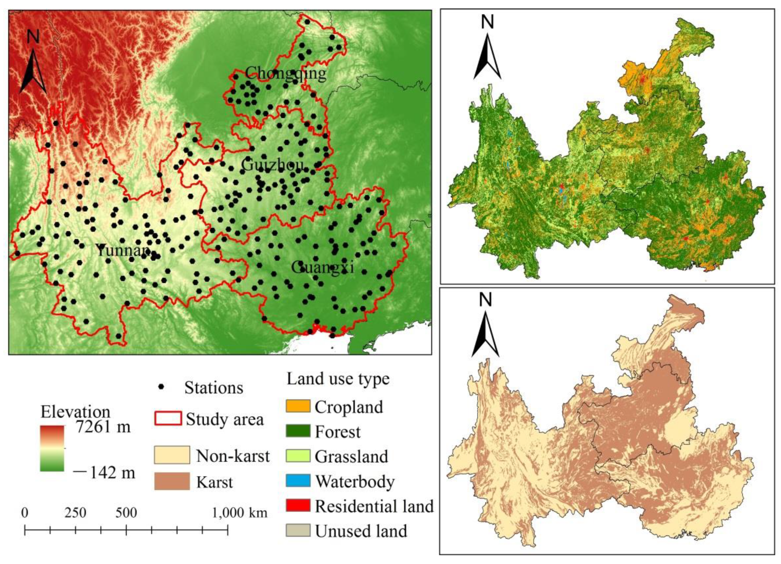
The study area is a typical karst landscape in Guizhou, Yunnan, Chongqing, and Guangxi provinces, southwestern China. It is mainly dominated by the karst plateau, karst basin, karst trough valley, and karst peak-cluster depression, respectively (Figure 1). The terrain is very complex, with average elevations of 400–1200 m. The mean annual precipitation is 1100 mm and the mean annual temperature is 20 °C, which is typical for a subtropical monsoon climate [25]. After launching the Grain for Green Project, general vegetation greening was observed in southwest China [11]. With the acceleration of urbanization, the speed of urbanization was greater than that of vegetation restoration.
2.2. Data
2.2.1. Modis NDVI Dataset
The selected normalized difference vegetation index (NDVI) dataset from 2000 to 2019 was obtained from the National Aeronautics and Space Administration (NASA) MOD13A3 product (https://ladsweb.modaps.eosdis.nasa.gov/search/ (accessed on 14 April 2021)), and it was utilized to describe the dynamic variations in the vegetation. The product, with a spatial resolution of 1 km and a monthly temporal resolution, had been corrected for radiation, geometry, and atmosphere. To avoid interferences such as that of winter snow on the NDVI images, we only studied the vegetation growing season (April to September). The preprocessing, including projection conversion and resampling, was conducted using the MODIS Reprojection Tool (MRT). Then, the monthly NDVI images of the study area were extracted in ArcGIS10.
2.2.2. Climate Data
The data for the climate factors during 2000–2019, including the maximum temperature, minimum temperature, mean temperature, mean relative humidity, mean land surface temperature, total precipitation, and total sunshine duration, were provided by the Institute of Geographic Sciences and Natural Resources of the Chinese Academy of Sciences, and there were 294 meteorological stations in total. After excluding the sites with missing data, the rest of the individual missing data were replaced using the mean values for the same period during an adjacent year [25]. We obtained the monthly climate data using the statistical calculation method.
2.2.3. Human Activities Data
We used nighttime light to detect human activities. The nighttime light 2000–2019 time-series data were derived from the research results of Ma et al. [36]. This dataset overcomes the shortcomings that the original two types of nighttime light data (DMSP-OLS and VIIRS-SDR) cannot be used simultaneously. We processed and calculated the nighttime light values using ArcGIS 10.2.
2.2.4. Environmental Data
The digital elevation model (DEM) data, with a spatial resolution of 90 m, were downloaded from the Geospatial Data Cloud (http://www.gscloud.cn/ (accessed on 16 April 2021)), which was used to extract the elevation and slope data. The administrative boundary data were obtained from the National Basic Geographic Information System. We obtained the spatial distribution of the lithology from the Institute of Geographic Sciences and Natural Resources of the Chinese Academy of Sciences. The Harmonized World Soil Database contains worldwide soil composition information at a spatial resolution of 30 arcsec. Two soil parameters included the percentages of the clay soil and sandy soil components were extracted from the database using ArcGIS10.2 (http://www.fao.org/soils-portal/soil-survey/soil-maps-and-databases/harmonized-world-soil-database-v12/en/ (accessed on 16 April 2021)).
2.3. Methods
2.3.1. Pearson Correlation Analysis
We used Pearson correlation analysis to analyze the time-lagged responses of the karst NDVI to the climatic factors. The correlation coefficients ranged from −1 to 1. The NDVI and climatic factor datasets from 2000 to 2019 were selected. We explored the correlation between the NDVI (current month) and the climatic factors (current month or previous month). When the correlation coefficient between the NDVI and climatic factors (previous month) was greater than the correlation coefficient between the NDVI and climatic factors (current month), we concluded that the climatic factors have a time-lagged effect on the NDVI, and these factors were selected as the input factors of the models.
2.3.2. Back Propagation Neural Network
A back propagation neural network (BPNN) used was a multi-layer feedforward neural network trained using an error back propagation algorithm, and it consisted of an input layer, hidden layer, and an output layer. The information was input into the input layer and was then treated in each successive layer and transmitted to the output layer. The error was calculated from the output layer and propagated to the input layer using a back propagation algorithm in order to adjust the weights and thresholds. A single hidden layer network structure was set up in the BPNN model. The optimal numbers of neurons in the hidden layer were determined through repeated training of the network. The numbers of neurons in the input layer and the output layer were determined by the numbers of input factors and output factor, respectively. There was a neural network toolbox in MATLAB2019b, which including BPNN we used. It involves three functions, parameter setting function ‘newff’, the training function ‘train’, and the prediction function ‘sim’ [37]. The input and output of the kth neuron were as follows [38]:
where was the connection weight between the ith neuron and the kth neuron; was the activation function; was the threshold; and and were the input and output of the kth neuron, respectively.
2.3.3. Radial Basis Function Neural Network
The radial basis function neural network (RBFNN) used was a feedforward neural network with a single hidden layer, and it was composed of an input layer, a hidden layer, and an output layer. Different from the BPNN, it used the radial basis function as the activation function in the hidden layer [39]. Functions such as newrbe and newrb were commonly used to build RBFNN models. Newrbe is characterized by fast neural network creation, and a zero-error radial basis network can be designed in order to improve the prediction accuracy [40]. In this paper, we utilized the newrbe function to build the RBFNN model to predict NDVI, and the spreading factor was adjusted to improve the model’s performance. The output of neurons from the output layer was as follows:
where n was the number of hidden layer neurons; and were the center and weight corresponding to the ith hidden layer neurons; and represented the radial basis functions.
2.3.4. Random Forest
The random forest (RF) algorithm was based on a decision tree. The principle of the RF was that each tree was composed of a random subset. In the splitting process, all of the features were not considered by the model, but the best feature was selected for the classification, which enriched the diversity of the decision trees in the model [41]. The algorithm was mainly divided into four steps. (1) The repeated sampling method was used to select a subset from all of the datasets as a training set. (2) The subset was used to build a decision tree. (3) The k decision trees were used to build the RF model by repeating the above steps k times. (4) The NDVI was predicted using the established RF model [41]. In this study, the RF model was developed using the treebagger function in regression model in MATLAB 2019b [42].
2.3.5. Support Vector Regression
Support vector regression (SVR) was developed by Vapnik in 1995, which was one of the most popular machine learning algorithms in capturing nonlinearity [43]. A kernel function was used to map the vectors into a higher dimensional feature space in the SVR model, and the model can be employed linear regression of the target variable in this space by introducing an alternative loss function and kernel function [44,45]. There were five commonly used kernel functions: the linear kernel function, the polynomial kernel function, the Gaussian kernel function, the Laplace kernel function, and the Sigmoid kernel function. The Gaussian kernel function is suitable for analyzing nonlinear relationships between influencing factors and the predicted factor [45], so we selected the Gaussian kernel function as the kernel function of the SVR model. For detailed information on the SVR model as seen Refs. [43,46]. The libsvm-3.24 toolbox was developed by Chang et al. [47] in 2011, and we constructed the SVR model using this toolbox. The process of predicting karst NDVI by machine learning methods was shown in Figure 2.
2.4. Assessment Criteria
To explore the prediction accuracy of the BPNN, RBFNN, RF, and SVR models, the statistical parameters including the coefficient of determination (R2), mean square error (MSE), root mean square error (RMSE), and mean absolute percentage error (MAPE) were used to calculate in different karst NDVI prediction results (Karst plateau, Karst basin, Karst trough valley, Karst peak-cluster depression). The higher the R2 value and the lower the MSE, RMSE, and MAPE values were, the better the model’s prediction performance was. The formulas for the assessment criteria were as follows:
where n was the sample number of validation period; and and were the predicted and observed NDVI, respectively.
2.5. Data Pre-Processing
The data were divided into training sets (from 2000 to 2011) and validation sets (from 2012 to 2019) using a ratio segmentation 6:4. Based on the MATLAB 2019b software, a nonlinear relationship model between the NDVI and the response factors was built and the karst NDVI was predicted. To keep the different units and magnitude of the factors from affecting the model’s performance, the input data were normalized to within a range of [0, 1] before being fed into the model [48].
where was the normalized data; was the observed data; and and were the minimum and maximum of the data, respectively.
3. Results
3.1. BPNN Model
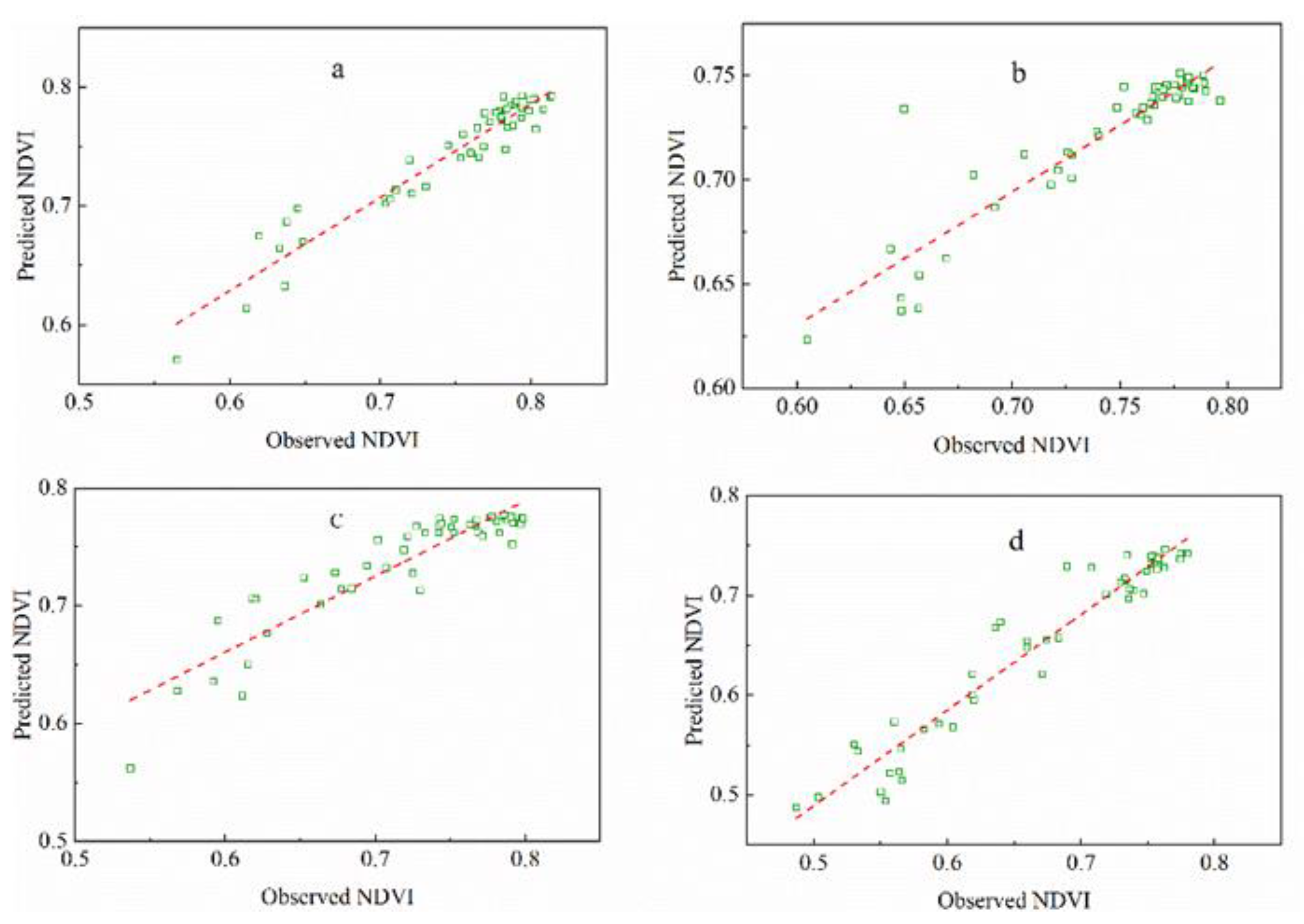
We obtained the BPNN network structures of the NDVI prediction models (the number of neurons in the input layer—the number of neurons in the hidden layer—the number of neurons in the output layer) in the karst plateau, karst basin, karst trough valley, and karst peak-cluster depression areas, which were 18-1-1, 29-4-1, 22-1-1, and 23-3-1, respectively. The R2 values of the results ranged from 0.6327 to 0.8713, with an average of 0.7744 (Table 1). The ranges of the MSE, RMSE, and MAPE values were 0.0007–0.0022, 0.0241–0.0452, and 2.4604–5.6112, respectively, with averages of 0.0017, 0.0384, and 4.4570, respectively, which indicate that the BPNN model is acceptable for karst NDVI prediction. In the NDVI model prediction of karst trough valley, the model’s generalization performance was better than those of the other karst NDVI prediction models (Figure 3).
3.2. RBFNN Model
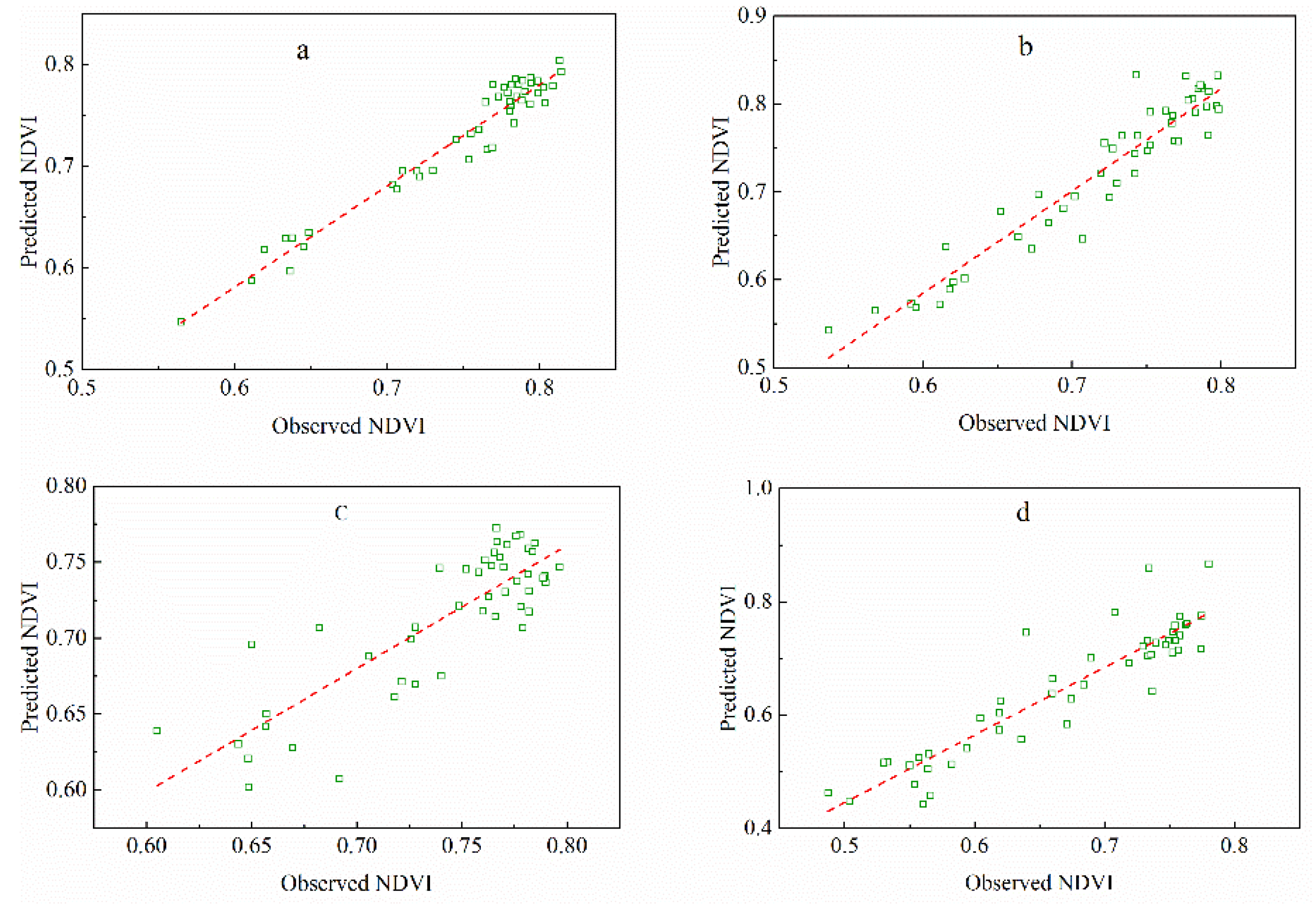
The R2 values were 0.7201–0.9516, with an average of 0.8563 (Table 2). The ranges of the MSE, RMSE, and MAPE values were 0.0006–0.0027, 0.0238–0.0520, and 2.6835–6.1581, respectively, with averages of 0.0014, 0.0356, and 4.1107, respectively. In the karst trough valley NDVI prediction, the model’s accuracy had a better performance than the other karst NDVI predictions (Figure 4). By comparing the R2, MSE, RMSE, and MAPE values to those of the BPNN, we concluded that the prediction accuracy of the RBFNN was higher than that of the BPNN.
3.3. RF Model
The optimal numbers of leaf nodes and trees (5 and 1000, respectively) were determined to achieve the best prediction accuracy of the RF model. The R2 values were 0.8136–0.9422, with an average of 0.8919 (Table 3). The MSE, RMSE, and MAPE values were 0.0012–0.0030, 0.0346–0.0546, and 4.3629–6.8243, respectively, with averages of 0.0023, 0.0468, and 5.8686, respectively. In the karst basin and karst trough valley NDVI predictions, the R2 values were up to 0.9422 and 0.9329, respectively, indicating that the model performed better in these regions than in the other karst NDVI predictions (Figure 5). The errors of the validation period were lower, and the prediction accuracy of the RF was good.
3.4. SVR Model
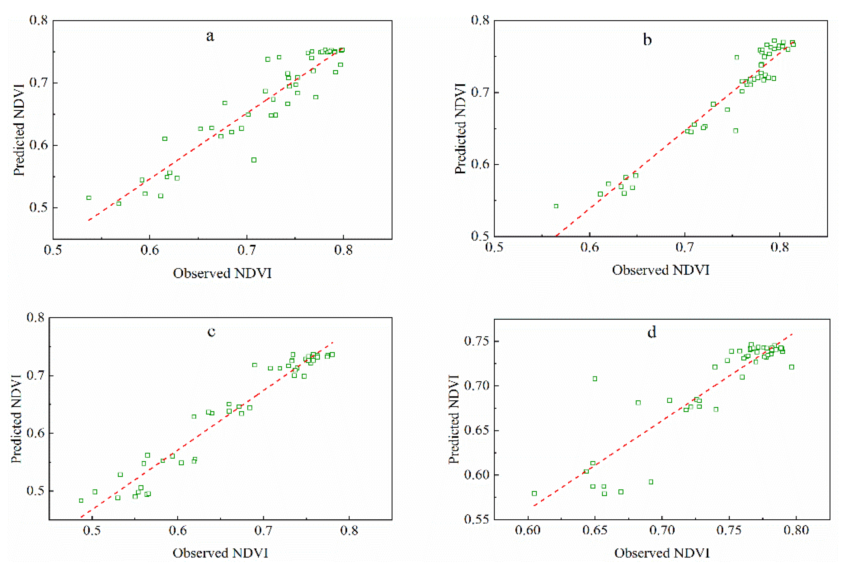
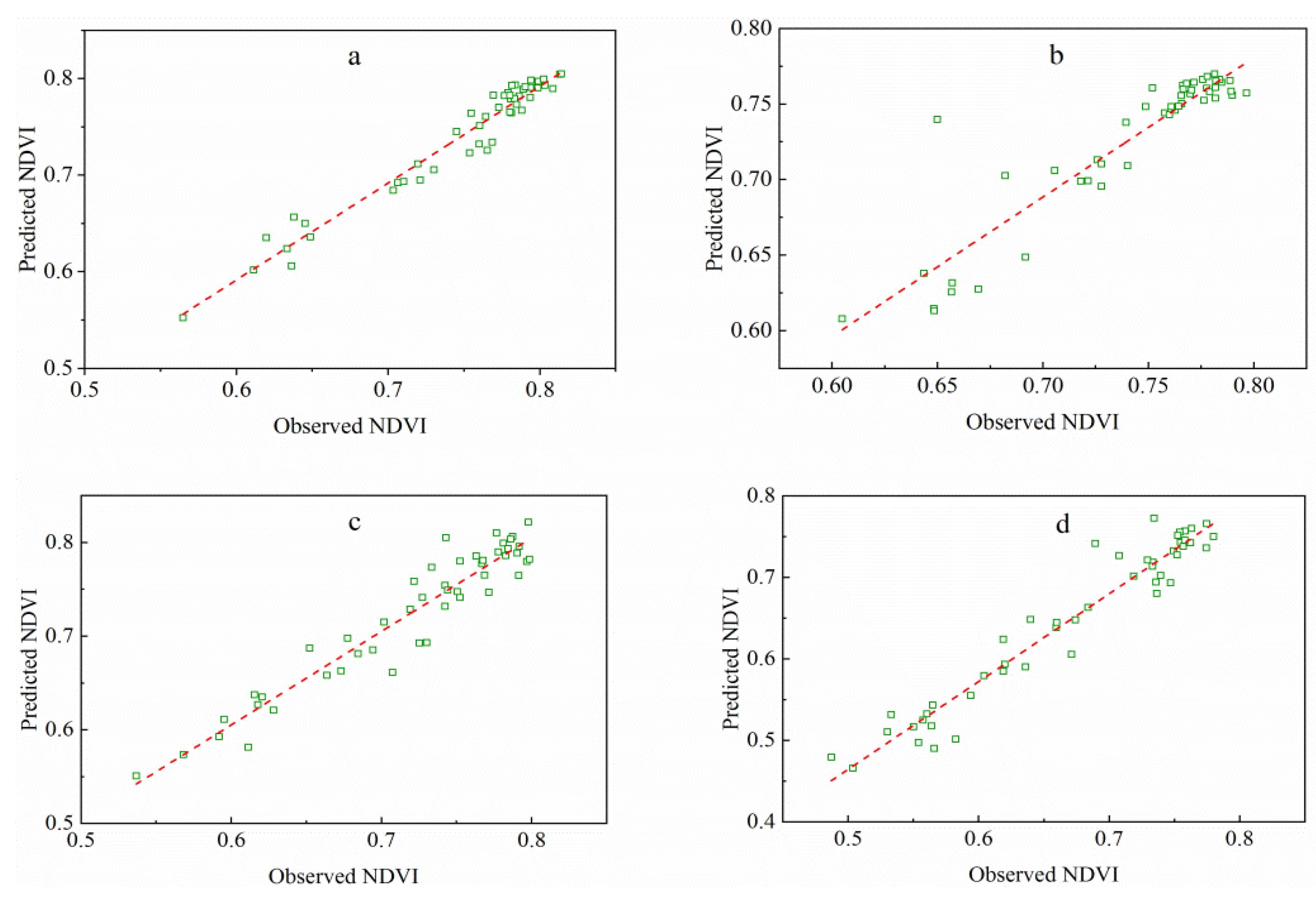
The R2 values were 0.8427–0.9564, with an average of 0.9128 (Table 4). The model prediction accuracy was greater than 0.9 in the study area, except for the karst peak-cluster depression NDVI prediction. The MSE, RMSE, and MAPE values were 0.0002–0.0011, 0.0154–0.0336, and 1.6700–4.2682, respectively, with averages of 0.0006, 0.0239, and 2.7732, respectively. The model performed the best overall in the karst trough valley NDVI prediction compared to in the other regions. This shows that the SVR model had a higher accuracy in the karst NDVI prediction (Figure 6).
3.5. Comparison of Prediction Results
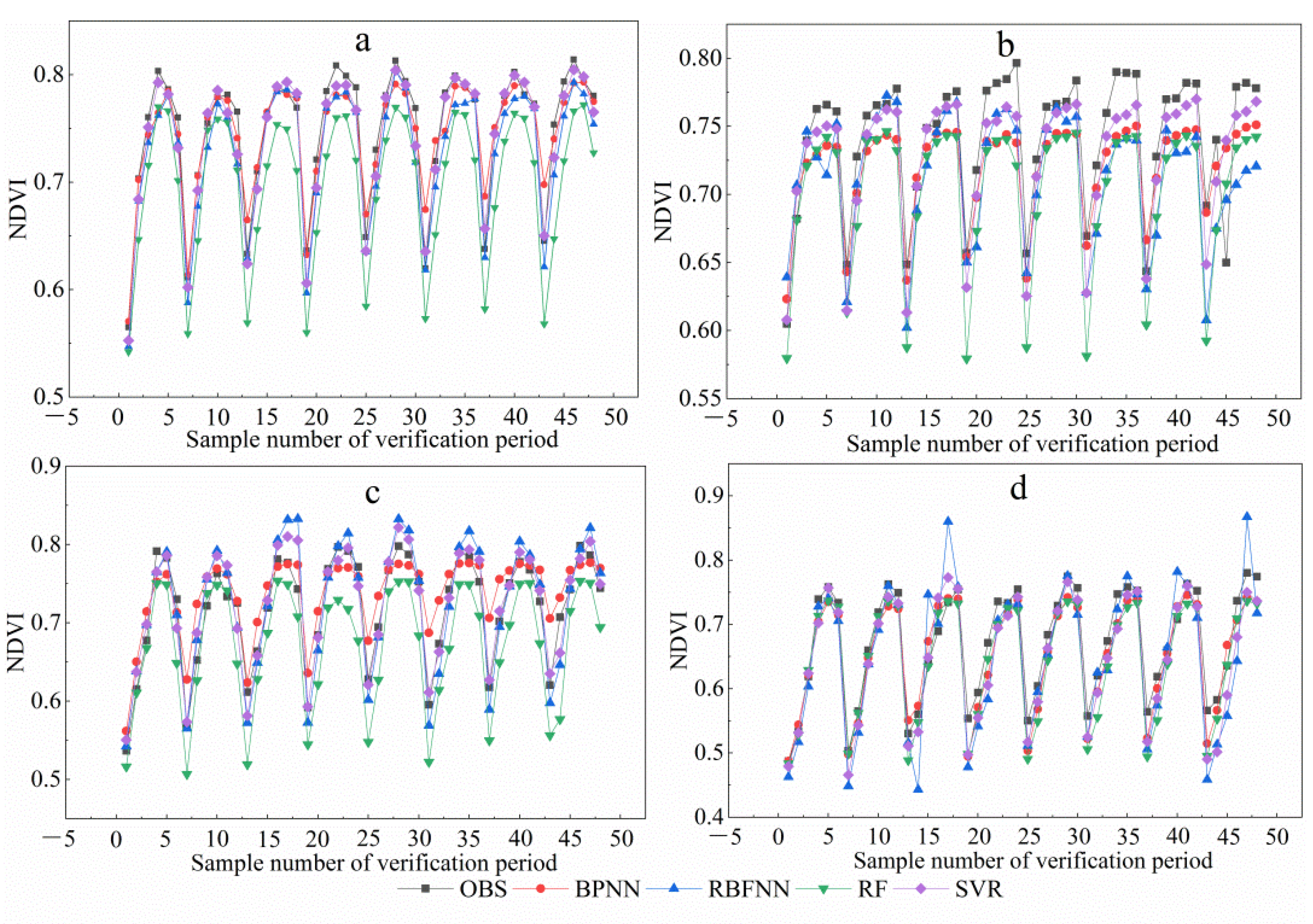
The comparison of the karst NDVI prediction results of the different models is shown in Figure 7 and Figure 8. In the karst trough valley NDVI prediction, the R2 values were SVR > RBFNN > RF > BPNN, and the MSE and RMSE values were SVR < RBFNN < BPNN < RF, while the MAPE values were SVR < BPNN < RBFNN < RF. In the karst peak-cluster depression NDVI prediction, the R2 values were SVR > RF > RBFNN > BPNN, and the errors were SVR < RBFNN < BPNN < RF. In the karst plateau NDVI prediction, the R2 values were SVR > RBFNN > RF > BPNN, and the errors were SVR < RBFNN < BPNN < RF. In the karst basin NDVI prediction, the R2 values were RF > SVR > RBFNN > BPNN, and the errors were SVR < RF < BPNN < RBFNN. The prediction accuracy of the SVR was higher than those of the other models, while its MSE, RMSE, and MAPE values were lower than those of the other models. Thus, we conclude that the SVR model is more suitable for karst NDVI prediction.
4. Discussion
Several scholars have studied the response of the vegetation NDVI to impact factors and have analyzed its changes in southwestern China. However, they did not distinguish between karst vegetation and non-karst vegetation, resulting in inadequately reflecting the nonlinear relationship between the karst vegetation and the impact factors in this special geologic environment. Vegetation growth is not affected by a single factor but is the result of the combined effect of multiple factors. Compared to non-karst vegetation, karst vegetation is more affected by topography, climate, and human activity factors [9]. Karst vegetation is significantly affected by both climate and non-climate factors, and the response of vegetation to climate exhibits nonlinear characteristics and compound effects [26]. Previous studies have concluded that the relationship between the land surface temperature and the NDVI has opposite spatial distribution patterns in typical karst regions at the macroscopic and microscopic levels [49]. Vegetation activities can be regulated by moisture changes, but increased moisture may inhibit vegetation activities due to increased cloud cover and relative humidity [26]. Wang et al. [13] found that temperature and precipitation have larger impacts on the NDVI than the annual sunshine duration. The present climatic conditions may not be the primary driving factor of vegetation growth, and the earlier climatic conditions may be the most important factors affecting vegetation growth. By determining the time-lag effect, we can better predict and evaluate vegetation dynamics under the background of global climate change [50]. Thus, the time-lag effects of the climate factors on vegetation play a non-negligible role in vegetation prediction. The topography can explain the spatial distribution characteristics of the vegetation cover to a certain extent. Different soil textures have a significant effect on karst vegetation. Increasing the percentage of the sandy soil component will progressively improve the direct response of the vegetation to drought, while increasing the percentage of the clay soil component will have the opposite effect [15]. Therefore, using a suitable nonlinear method to predict karst vegetation based on multiple factors could enhance the explanation of the nonlinear process of vegetation growth.
Linear methods are currently the most commonly used methods of analyzing karst vegetation changes, but the variable interactions are hard to be considered, resulting in difficulty revealing the nonlinear relationships between predict and response factors [25]. The response of vegetation to the influencing factors is complex and nonlinear. Machine learning methods are very effective in dealing with nonlinear relationships between the system’s inputs and outputs. They can speculate and improve algorithms independently and enhance the accuracy and efficiency by obtaining experience [28]. With machine learnings, we can better reveal the nonlinear relationship of vegetation greening with natural and human activities factors and for better prediction. The karst NDVI prediction results of the BPNN, RBFNN, RF, and SVR models are presented in Table 1, Table 2, Table 3 and Table 4. The mean R2 values were 0.7744, 0.8563, 0.8919, and 0.9128, respectively. Based on the assessment of errors, the models were within the acceptable ranges. Wu et al. [16] have employed four modeling approaches: linear regression, generalized additive models, support vector machine, and RF to fit vegetation cover change, the results obtained that the RF model produced the highest accuracy and lowest error. Four supervised machine algorithms: SVR, RF, linear and polynomial regression were used to predict NDVI and EVI, the results showed that the RF model for NDVI and EVI prediction have high levels of accuracy [35]. Different from the above research, our research found the SVR model has the lowest errors and the highest accuracy compared with the BPNN, RBFNN, and RF models, which was indicating that the SVR model was the best for karst vegetation prediction.
From the perspective of the principle of these models, the gradient descent method is widely used to adjust the weights of the BPNN neurons, but its limitations are a slow convergence speed and being easy to fall to a local optimum [39], which result in a relatively poor prediction accuracy. The ability of the RBFNN model to produce global approximations could solve the local optimum problem of the BPNN model, so its vegetation prediction approximation accuracy is obviously higher than that of the BP [39]. The data input into the RF model was divided into intervals to yield the mean results for each interval, which makes the RF model very flexible [51]. The advantages of the SVR model are the uniqueness and global optimality of the generated solution [52] and it determines the maximum-margin hyperplane [53], which improves the prediction accuracy and reduces the prediction error. However, the interpretation of most machine learning algorithms is often considered hard, similar to a black box [54]. Without an explicit regression equation for the final model, the resulting input-output relationships from the black box model cannot be provided good interpretability [25]. However, machine learning algorithms still have powerful functions in dealing with complex nonlinear relationships. In this study, the RBFNN and RF models had relatively higher accuracies, but they were significantly biased compared to the performance of the SVR model.
In this study, we only predicted the NDVI in the growing season in typical karst regions and discussed the optimal machine learning method for karst NDVI prediction. It is relatively rough to extract data, such as topography and soil texture data, from on the regional scale because of the strong landscape heterogeneity in karst areas. In addition, MODIS NDVI time-series data have a relatively low spatial resolution. The karst region is characterized by a high bedrock exposure and low vegetation coverage. The prediction results may be influenced by the spectral response of the ground. In the future, we will explore the dynamic changes in the karst vegetation on multiple time scales and grid-in-grid distribution scales. Applying machine learning methods to accurately predict karst vegetation at multiple temporal and spatial scales in order to provide a scientific basis for karst vegetation restoration and environmental governance is very important.
5. Conclusions
In this study, we selected relevant climate, human activity, soil texture, and topography factors. The BPNN, RBFNN, RF, and SVR methods were employed to construct a nonlinear relationship model between the karst NDVI and these factors and then to predict the karst NDVI. Pearson correlation analysis was used to analyze and select the climate factors, which had a time-lagged effect on the NDVI, influencing the NDVI as inputs of the model. By assessing the model performance, we determined the best model for vegetation prediction.
By assessing the models using the mean R2 values as the criteria, it was found that the observed values agree well with the predicted values for the BPNN, RBFNN, RF, and SVR models (R2: 0.77, 0.86, 0.89, and 0.91, respectively). Based on the mean MSE, RMSE, and MAPE values (MSE: 0.002, 0.001, 0.002, and 0.001; RMSE: 0.04, 0.04, 0.05, and 0.02; MAPE: 4.46, 4.11, 5.87, and 2.77, respectively), the models are within the acceptable range.
By comparing the models’ results (R2, MSE, RMSE, and MAPE), it was determined that the models are acceptable for karst NDVI prediction. Although the prediction accuracy of the RF model for the karst basin NDVI was higher than that of the SVR model, the overall errors of the SVR model were lower than those of the RF model. The results show that the SVR model significantly outperformed the BPNN, RBFNN, and RF models in terms of the standard statistical indexes, and thus, it is more suitable for karst NDVI prediction. The accuracy of the SVR model is affected by the different parameters; and a well-trained SVR model is a useful tool for predicting karst vegetation. Our results can provide references for vegetation prediction in karst areas and more accurate predictions for the assessment of ecological evolution.
Author Contributions
Conceptualization, Y.M., J.G. and L.Z.; methodology, Y.M. and Q.L.; software, Y.M.; validation, Y.M.; formal analysis, Y.M., J.G. and L.Z.; investigation, Y.M. and Q.L.; resources, L.Z., L.L., Y.M. and J.G.; data curation, Y.M., L.Z., L.L. and J.G.; writing—original draft preparation, Y.M.; writing—review and editing, Y.M. and L.Z.; visualization, Y.M., J.G. and L.Z.; supervision, J.G.; project administration, J.G.; funding acquisition, J.G. All authors have read and agreed to the published version of the manuscript.
Funding
This research was funded by the National Natural Science Foundation of China, grant number 42071288 and 41671098; the Programme of Kezhen-Bingwei Excellent Young Scientists of the Institute of Geographic Sciences and Natural Resources Research, Chinese Academy of Sciences, grant number 2020RC002; the National Key Research and Development Program of China, grant number 2018YFC1509002.
Institutional Review Board Statement
Not applicable.
Informed Consent Statement
Not applicable.
Data Availability Statement
Not applicable.
Conflicts of Interest
The authors declare no conflict of interest.
References
- Liu, M.X.; Xu, X.L.; Wang, D.B.; Sun, A.Y.; Wang, K.L. Karst catchments exhibited higher degradation stress from climate change than the non-karst catchments in southwest China: An ecohydrological perspective. J. Hydrol. 2016, 535, 173–180. [Google Scholar] [CrossRef]
- Liu, C.C.; Liu, Y.G.; Guo, K.; Zhao, H.W.; Qiao, X.G.; Wang, S.J.; Zhang, L.; Cai, X.L. Mixing litter from deciduous and evergreen trees enhances decomposition in a subtropical karst forest in southwestern China. Soil Biol. Biochem. 2016, 101, 44–54. [Google Scholar] [CrossRef]
- Liu, C.C.; Liu, Y.G.; Guo, K.; Wang, S.J.; Liu, H.M.; Zhao, H.W.; Qiao, X.G.; Hou, D.J.; Li, S.B. Aboveground carbon stock, allocation and sequestration potential during vegetation recovery in the karst region of southwestern China: A case study at a watershed scale. Agric. Ecosyst. Environ. 2016, 235, 91–100. [Google Scholar] [CrossRef]
- Fan, F.D.; Wang, K.L.; Xiong, Y.; Xuan, Y.; Zhang, W.; Yue, Y.M. Assessment and spatial distribution of water and soil loss in karst regions, southwest China. Acta Ecol. Sin. 2011, 31, 6353–6362, (In Chinese with English abstract). [Google Scholar]
- Wu, L.H.; Wang, S.J.; Bai, X.Y.; Tian, Y.C.; Luo, G.J.; Wang, J.F.; Li, Q.; Chen, F.; Deng, Y.H.; Yang, Y.J. Climate change weakens the positive effect of human activities on karst vegetation productivity restoration in southern China. Ecol. Indic. 2020, 115, 106392. [Google Scholar] [CrossRef]
- Deng, Y.H.; Wang, S.J.; Bai, X.Y.; Luo, G.J.; Wu, L.H.; Chen, F.; Wang, J.F.; Li, C.J.; Yang, Y.J.; Hu, Z.Y. Vegetation greening intensified soil drying in some semi-arid and arid areas of the world. Agric. For. Meteorol. 2020, 292, 108103. [Google Scholar] [CrossRef]
- Yuan, L.H.; Chen, X.Q.; Wang, X.Y.; Xiong, Z.; Song, C.Q. Spatial associations between NDVI and environmental factors in the Heihe River Basin. J. Geogr. Sci. 2019, 29, 1548–1564. [Google Scholar] [CrossRef] [Green Version]
- Zhang, X.M.; Yue, Y.M.; Tong, X.W.; Wang, K.L.; Qi, X.K.; Deng, C.X.; Brandt, M. Eco-engineering controls vegetation trends in southwest China karst. Sci. Total Environ. 2021, 770, 145160. [Google Scholar] [CrossRef] [PubMed]
- Xiao, J.Y.; Wang, S.J.; Bai, X.Y.; Zhou, D.Q.; Tian, Y.C.; Li, Q.; Wu, L.H.; Qian, Q.H.; Chen, F.; Zeng, C. Determinants and spatial-temporal evolution of vegetation coverage in the karst critical zone of South China. Acta Ecol. Sin. 2018, 38, 8799–8812, (In Chinese with English abstract). [Google Scholar]
- Tong, X.W.; Wang, K.L.; Yue, Y.M.; Brandt, M.; Liu, B.; Zhang, C.H.; Liao, C.J.; Fensholt, R. Quantifying the effectiveness of ecological restoration projects on long-term vegetation dynamics in the karst regions of Southwest China. Int. J. Appl. Earth Obs. Geoinf. 2017, 54, 105–113. [Google Scholar] [CrossRef] [Green Version]
- Qiao, Y.N.; Jiang, Y.J.; Zhang, C.Y. Contribution of karst ecological restoration engineering to vegetation greening in southwest China during recent decade. Ecol. Indic. 2021, 121, 107081. [Google Scholar] [CrossRef]
- Jiang, Z.; Liu, H.Y.; Wang, H.Y.; Peng, J.; Meersmans, J.; Green, S.M.; Quine, T.A.; Wu, X.C.; Song, Z.L. Bedrock geochemistry influences vegetation growth by regulating the regolith water holding capacity. Nat. Commun. 2020, 11, 2392. [Google Scholar] [CrossRef]
- Wang, J.; Wang, K.L.; Zhang, M.Y.; Zhang, C.H. Impacts of climate change and human activities on vegetation cover in hilly southern China. Ecol. Eng. 2015, 81, 451–461. [Google Scholar] [CrossRef]
- Sun, C.F.; Liu, Y.; Song, H.M.; Cai, Q.F.; Li, Q.; Wang, L.; Mei, R.C.; Fang, C.X. Sunshine duration reconstruction in the southeastern Tibetan Plateau based on tree-ring width and its relationship to volcanic eruptions. Sci. Total Environ. 2018, 628–629, 707–714. [Google Scholar] [CrossRef]
- Jiang, P.; Ding, W.G.; Yuan, Y.; Ye, W.F. Diverse response of vegetation growth to multi-time-scale drought under different soil textures in China’s pastoral areas. J. Environ. Manag. 2020, 274, 110992. [Google Scholar] [CrossRef]
- Qiao, Y.N.; Chen, H.; Jiang, Y.J. Quantifying the impacts of lithology on vegetation restoration using a random forest model in a karst trough valley, China. Ecol. Eng. 2020, 156, 105973. [Google Scholar] [CrossRef]
- Chen, T.T.; Peng, L.; Liu, S.Q.; Wang, Q. Land cover change in different altitudes of Guizhou-Guangxi karst mountain area, China: Patterns and drivers. J. Mt. Sci. 2017, 14, 1873–1888. [Google Scholar] [CrossRef]
- Zhou, Q.W.; Wei, X.C.; Zhou, X.; Cai, M.Y.; Xu, Y.X. Vegetation coverage change and its response to topography in a typical karst region: The Lianjiang River Basin in Southwest China. Environ. Earth Sci. 2019, 78, 191. [Google Scholar] [CrossRef]
- Yang, L.; Shen, F.X.; Zhang, L.; Cai, Y.Y.; Yi, F.X.; Zhou, C.H. Quantifying influences of natural and anthropogenic factors on vegetation changes using structural equation modeling: A case study in Jiangsu Province, China. J. Clean. Prod. 2021, 280, 124330. [Google Scholar] [CrossRef]
- Zhou, Y.Y.; Fu, D.J.; Lu, C.X.; Xu, X.M.; Tang, Q.H. Positive effects of ecological restoration policies on the vegetation dynamics in a typical ecologically vulnerable area of China. Ecol. Eng. 2021, 159, 106087. [Google Scholar] [CrossRef]
- Sun, Y.L.; Shan, M.; Pei, X.R.; Zhang, X.K.; Yang, Y.L. Assessment of the impacts of climate change and human activities on vegetation cover change in the Haihe River basin, China. Phys. Chem. Earth Parts A/B/C 2020, 115, 102834. [Google Scholar] [CrossRef]
- Zhou, Z.Q.; Ding, Y.B.; Shi, H.Y.; Cai, H.J.; Fu, Q.; Liu, S.N.; Li, T.X. Analysis and prediction of vegetation dynamic changes in China: Past, present and future. Ecol. Indic. 2020, 117, 106642. [Google Scholar] [CrossRef]
- Zarei, A.; Asadi, E.; Ebrahimi, A.; Jafari, M.; Malekian, A.; Nasrabadi, H.M.; Chemura, A.; Maskell, G. Prediction of future grassland vegetation cover fluctuation under climate change scenarios. Ecol. Indic. 2020, 119, 106858. [Google Scholar] [CrossRef]
- Zhang, Y.L.; Gao, J.G.; Liu, L.S.; Wang, Z.F.; Ding, M.J.; Yang, X.C. NDVI-based vegetation changes and their responses to climate change from 1982 to 2011: A case study in the Koshi River Basin in the middle Himalayas. Glob. Planet. Chang. 2013, 108, 139–148. [Google Scholar] [CrossRef]
- Liu, H.Y.; Jiao, F.S.; Yin, J.Q.; Li, T.Y.; Gong, H.B.; Wang, Z.Y.; Lin, Z.S. Nonlinear relationship of vegetation greening with nature and human factors and its forecast—A case study of Southwest China. Ecol. Indic. 2020, 111, 106009. [Google Scholar] [CrossRef]
- Gao, J.B.; Jiao, K.W.; Wu, S.H. Investigating the spatially heterogeneous relationships between climate factors and NDVI in China during 1982 to 2013. J. Geogr. Sci. 2019, 29, 1597–1609. [Google Scholar] [CrossRef] [Green Version]
- Tian, Y.C.; Bai, X.Y.; Wang, S.J.; Qin, L.Y.; Li, Y. Spatial-temporal changes of vegetation cover in Guizhou Province, Southern China. Chin. Geogr. Sci. 2017, 27, 25–38. [Google Scholar] [CrossRef] [Green Version]
- Mahmoodzadeh, A.; Mohammadi, M.; Ali, H.F.H.; Abdulhamid, S.N.; Ibrahim, H.H.; Noori, K.M.G. Dynamic prediction models of rock quality designation in tunneling projects. Transp. Geotech. 2021, 27, 100497. [Google Scholar] [CrossRef]
- Vangeepuram, N.; Liu, B.; Chiu, P.H.; Wang, L.H.; Pandey, G. Predicting youth diabetes risk using NHANES data and machine learning. Sci. Rep. 2021, 11, 11212. [Google Scholar] [CrossRef]
- Hirano, Y.; Kondo, Y.; Hifumi, T.; Yokobori, S.; Kanda, J.; Shimazaki, J.; Hayashida, K.; Moriya, T.; Yagi, M.; Takauji, S. Machine learning-based mortality prediction model for heat-related illness. Sci. Rep. 2021, 11, 9501. [Google Scholar] [CrossRef]
- Wardeh, M.; Blagrove, M.S.C.; Sharkey, K.J.; Baylis, M. Divide-and-conquer: Machine-learning integrates mammalian and viral traits with network features to predict virus-mammal associations. Nat. Commun. 2021, 12, 3954. [Google Scholar] [CrossRef] [PubMed]
- Lewis, J.E.; Kemp, M.L. Integration of machine learning and genome-scale metabolic modeling identifies multi-omics biomarkers for radiation resistance. Nat. Commun. 2021, 12, 2700. [Google Scholar] [CrossRef] [PubMed]
- Peng, P.A.; He, Z.X.; Wang, L.; Jiang, Y.J. Microseismic records classification using capsule network with limited training samples in underground mining. Sci. Rep. 2020, 10, 13925. [Google Scholar] [CrossRef] [PubMed]
- Hounkpatin, K.O.L.; Schmidt, K.; Stumpf, F.; Forkuor, G.; Behrens, T.; Scholten, T.; Amelung, W.; Welp, G. Predicting reference soil groups using legacy data: A data pruning and Random Forest approach for tropical environment (Dano catchment, Burkina Faso). Sci. Rep. 2018, 8, 9959. [Google Scholar] [CrossRef]
- Roy, B. Optimum machine learning algorithm selection for forecasting vegetation indices: MODIS NDVI & EVI. Remote. Sens. Appl. Soc. Environ. 2021, 23, 100582. [Google Scholar]
- Ma, J.J.; Guo, J.Y.; Ahmad, S.; Li, Z.Q.; Hong, J. Constructing a New Inter-Calibration Method for DMSP-OLS and NPP-VIIRS Nighttime Light. Remote Sens. 2020, 12, 937. [Google Scholar] [CrossRef] [Green Version]
- Zhang, L.H.; Chao, B.; Zhang, X. Modeling and optimization of microbial lipid fermentation from cellulosic ethanol wastewater by Rhodotorula glutinis based on the support vector machine. Bioresour. Technol. 2020, 301, 122781. [Google Scholar] [CrossRef]
- Liu, S.Y.; Xu, L.Q.; Li, D.L. Multi-scale prediction of water temperature using empirical mode decomposition with back-propagation neural networks. Comput. Electr. Eng. 2016, 49, 1–8. [Google Scholar] [CrossRef]
- Du, B.; Lund, P.D.; Wang, J.; Kolhe, M.; Hu, E. Comparative study of modelling the thermal efficiency of a novel straight through evacuated tube collector with MLR, SVR, BP and RBF methods. Sustain. Energy Technol. Assess. 2021, 44, 101029. [Google Scholar]
- Zhou, T.J.; Ding, L.; Ji, J.; Yu, L.X.; Wang, Z. Combined estimation of fire perimeters and fuel adjustment factors in FARSITE for forecasting wildland fire propagation. Fire Saf. J. 2020, 116, 103167. [Google Scholar] [CrossRef]
- Wang, D.; Zhu, A.X. Soil Mapping Based on the Integration of the Similarity-Based Approach and Random Forests. Land 2020, 9, 174. [Google Scholar] [CrossRef]
- Lo, F.; Bitz, C.M.; Hess, J.J. Development of a Random Forest model for forecasting allergenic pollen in North America. Sci. Total Environ. 2021, 773, 145590. [Google Scholar] [CrossRef]
- Shen, M.; Sun, H.Y.; Lu, Y.J. Household Electricity Consumption Prediction Under Multiple Behavioural Intervention Strategies Using Support Vector Regression. Energy Procedia 2017, 142, 2734–2739. [Google Scholar] [CrossRef]
- Shi, Y. Support vector regression-based QSAR models for prediction of antioxidant activity of phenolic compounds. Sci. Rep. 2021, 11, 8806. [Google Scholar] [CrossRef] [PubMed]
- Hong, W.C. Electric load forecasting by seasonal recurrent SVR (support vector regression) with chaotic artificial bee colony algorithm. Energy 2011, 36, 5568–5578. [Google Scholar] [CrossRef]
- Cheng, K.; Lu, Z.Z.; Zhou, Y.C.; Shi, Y.; Wei, Y.H. Global sensitivity analysis using support vector regression. Appl. Math. Model. 2017, 49, 587–598. [Google Scholar] [CrossRef]
- Chang, C.C.; Lin, C.J. Libsvm. ACM Trans. Intell. Syst. Technol. 2011, 2, 1–27. [Google Scholar] [CrossRef]
- Mohammadi, B.; Mehdizadeh, S. Modeling daily reference evapotranspiration via a novel approach based on support vector regression coupled with whale optimization algorithm. Agric. Water Manag. 2020, 237, 106145. [Google Scholar] [CrossRef]
- Deng, Y.H.; Wang, S.J.; Bai, X.Y.; Tian, Y.C.; Wu, L.H.; Xiao, J.Y.; Chen, F.; Qian, Q.H. Relationship among land surface temperature and LUCC, NDVI in typical karst area. Sci. Rep. 2018, 8, 641. [Google Scholar] [CrossRef] [PubMed]
- Wu, D.H.; Zhao, X.; Liang, S.L.; Zhou, T.; Huang, K.C.; Tang, B.J.; Zhao, W.Q. Time-lag effects of global vegetation responses to climate change. Glob. Chang. Biol. 2015, 21, 3520–3531. [Google Scholar] [CrossRef]
- de Souza, G.S.A.; Soares, V.P.; Leite, H.G.; Gleriani, J.M.; do Amaral, C.H.; Ferraz, A.S.; Silveira, M.V.D.; dos Santos, J.F.C.; Velloso, S.G.S.; Domingues, G.F. Multi-sensor prediction of Eucalyptus stand volume: A support vector approach. ISPRS J. Photogramm. Remote Sens. 2019, 156, 135–146. [Google Scholar] [CrossRef]
- Wang, R.; Lu, S.L.; Li, Q.P. Multi-criteria comprehensive study on predictive algorithm of hourly heating energy consumption for residential buildings. Sustain. Cities Soc. 2019, 49, 101623. [Google Scholar] [CrossRef]
- Krishna, G.; Sahoo, R.N.; Singh, P.; Bajpai, V.; Patra, H.; Kumar, S.; Dandapani, R.; Gupta, V.K.; Viswanathan, C.; Ahmad, T. Comparison of various modelling approaches for water deficit stress monitoring in rice crop through hyperspectral remote sensing. Agric. Water Manag. 2019, 213, 231–244. [Google Scholar] [CrossRef]
- Doornenbal, B.M.; Spisak, B.R.; van der Laken, P.A. Opening the black box: Uncovering the leader trait paradigm through machine learning. Leadersh. Q. 2021, 101515. [Google Scholar] [CrossRef]
Figure 1.
The distribution of the karst area and land use types in the study region.

Figure 2.
Architecture of the prediction framework using machine learning methods.

Figure 3.
Comparison of the observed and BPNN predicted NDVI in the (a) karst trough valley, (b) karst peak-cluster depression, (c) karst plateau, and (d) karst basin.
Figure 3.
Comparison of the observed and BPNN predicted NDVI in the (a) karst trough valley, (b) karst peak-cluster depression, (c) karst plateau, and (d) karst basin.

Figure 4.
Comparison of the observed and RBFNN predicted NDVI in the (a) karst trough valley, (b) karst plateau, (c) karst peak-cluster depression, and (d) karst basin.
Figure 4.
Comparison of the observed and RBFNN predicted NDVI in the (a) karst trough valley, (b) karst plateau, (c) karst peak-cluster depression, and (d) karst basin.

Figure 5.
Comparison of the observed and RF predicted NDVI in the (a) karst plateau, (b) karst trough valley, and (c) karst basin, (d) karst peak-cluster depression.
Figure 5.
Comparison of the observed and RF predicted NDVI in the (a) karst plateau, (b) karst trough valley, and (c) karst basin, (d) karst peak-cluster depression.

Figure 6.
Comparison of the observed and SVR predicted NDVI in the (a) karst trough valley, (b) karst peak-cluster depression, (c) karst plateau, (d) and karst basin.
Figure 6.
Comparison of the observed and SVR predicted NDVI in the (a) karst trough valley, (b) karst peak-cluster depression, (c) karst plateau, (d) and karst basin.

Figure 7.
Comparison of the observed and BPNN, RBFNN, RF, and SVR predicted NDVI in the (a) karst trough valley, (b) karst peak-cluster depression, (c) karst plateau, and (d) karst basin.
Figure 7.
Comparison of the observed and BPNN, RBFNN, RF, and SVR predicted NDVI in the (a) karst trough valley, (b) karst peak-cluster depression, (c) karst plateau, and (d) karst basin.

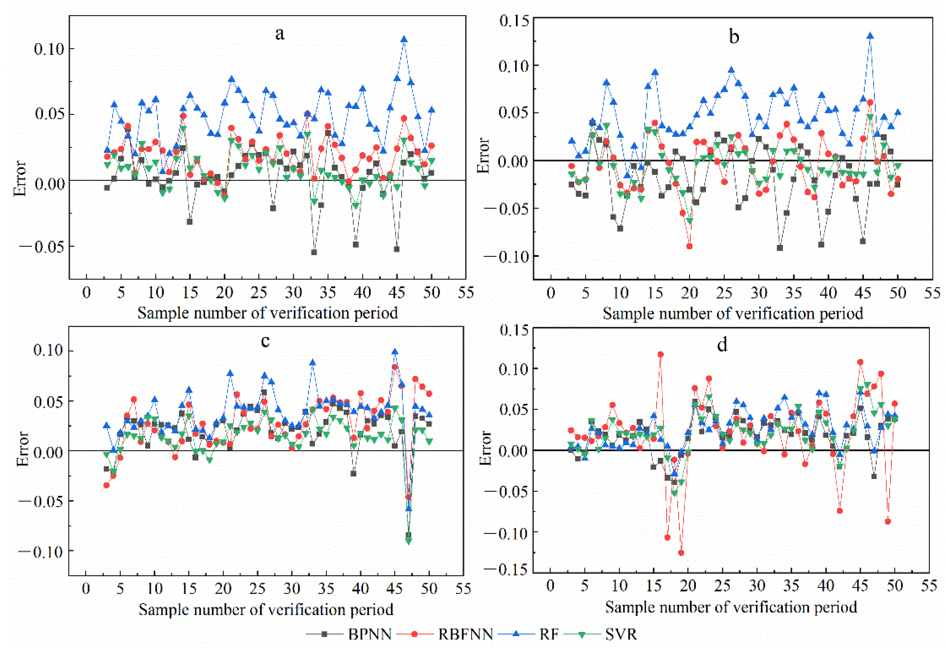
Figure 8.
Error of the BPNN, RBFNN, RF, and SVR for the predicted NDVI in the (a) karst trough valley, (b) karst plateau, (c) karst peak-cluster depression, and (d) karst basin.
Figure 8.
Error of the BPNN, RBFNN, RF, and SVR for the predicted NDVI in the (a) karst trough valley, (b) karst plateau, (c) karst peak-cluster depression, and (d) karst basin.


Table 1.
The prediction accuracy of the BPNN model.
| Karst Regions | R2 | MSE | RMSE | MAPE |
|---|---|---|---|---|
| Karst plateau | 0.7547 | 0.0021 | 0.0442 | 5.1697 |
| Karst basin | 0.8389 | 0.0022 | 0.0452 | 5.6112 |
| Karst trough valley | 0.8713 | 0.0007 | 0.0241 | 2.4604 |
| Karst peak-cluster depression | 0.6327 | 0.0017 | 0.0400 | 4.5865 |
Table 2.
The prediction accuracy of the RBFNN model.
| Karst Regions | R2 | MSE | RMSE | MAPE |
|---|---|---|---|---|
| Karst plateau | 0.9087 | 0.0008 | 0.0282 | 3.2034 |
| Karst basin | 0.8447 | 0.0027 | 0.0520 | 6.1581 |
| Karst trough valley | 0.9516 | 0.0006 | 0.0238 | 2.6835 |
| Karst peak-cluster depression | 0.7201 | 0.0015 | 0.0383 | 4.3979 |
Table 3.
The prediction accuracy of the RF model.
| Karst Regions | R2 | MSE | RMSE | MAPE |
|---|---|---|---|---|
| Karst plateau | 0.8790 | 0.0030 | 0.0546 | 6.8243 |
| Karst basin | 0.9422 | 0.0012 | 0.0346 | 4.3629 |
| Karst trough valley | 0.9329 | 0.0028 | 0.0525 | 6.6639 |
| Karst peak-cluster depression | 0.8136 | 0.0021 | 0.0453 | 5.6231 |
Table 4.
The prediction accuracy of the SVR model.
| Karst Regions | R2 | MSE | RMSE | MAPE |
|---|---|---|---|---|
| Karst plateau | 0.9150 | 0.0005 | 0.0218 | 2.4420 |
| Karst basin | 0.9370 | 0.0011 | 0.0336 | 4.2682 |
| Karst trough valley | 0.9564 | 0.0002 | 0.0154 | 1.6700 |
| Karst peak-cluster depression | 0.8427 | 0.0006 | 0.0248 | 2.7124 |
Publisher’s Note: MDPI stays neutral with regard to jurisdictional claims in published maps and institutional affiliations. |
© 2021 by the authors. Licensee MDPI, Basel, Switzerland. This article is an open access article distributed under the terms and conditions of the Creative Commons Attribution (CC BY) license (https://creativecommons.org/licenses/by/4.0/).
Share and Cite
MDPI and ACS Style
Ma, Y.; Zuo, L.; Gao, J.; Liu, Q.; Liu, L. Comparing Four Types Methods for Karst NDVI Prediction Based on Machine Learning. Atmosphere 2021, 12, 1341. https://0-doi-org.brum.beds.ac.uk/10.3390/atmos12101341
AMA Style
Ma Y, Zuo L, Gao J, Liu Q, Liu L. Comparing Four Types Methods for Karst NDVI Prediction Based on Machine Learning. Atmosphere. 2021; 12(10):1341. https://0-doi-org.brum.beds.ac.uk/10.3390/atmos12101341
Chicago/Turabian StyleMa, Yuju, Liyuan Zuo, Jiangbo Gao, Qiang Liu, and Lulu Liu. 2021. "Comparing Four Types Methods for Karst NDVI Prediction Based on Machine Learning" Atmosphere 12, no. 10: 1341. https://0-doi-org.brum.beds.ac.uk/10.3390/atmos12101341
Note that from the first issue of 2016, this journal uses article numbers instead of page numbers. See further details here.