Article

Land Surface Temperature Retrieval Using High-Resolution Vertical Profiles Simulated by WRF Model †

by
Lucas Ribeiro Diaz
1,2,*,
Daniel Caetano Santos
3,
Pâmela Suélen Käfer
1,
Nájila Souza da Rocha
1,
Savannah Tâmara Lemos da Costa
1,
Eduardo Andre Kaiser
1 and
Silvia Beatriz Alves Rolim
1
1
State Research Center for Remote Sensing and Meteorology (CEPSRM), Universidade Federal do Rio Grande do Sul (UFRGS), Av. Bento Gonçalves 9500, Porto Alegre 91501-970, RS, Brazil
2
Faculty of Science, Vrije Universiteit Amsterdam, de Boelelaan 1085, 1081 HV Amsterdam, The Netherlands
3
Center for Natural and Exact Sciences, Department of Physics, Universidade Federal de Santa Maria (UFSM), Av. Roraima, Santa Maria 97105-900, RS, Brazil
*
Author to whom correspondence should be addressed.
This paper is an expanded version of the work presented at the 4th International Electronic Conference on Atmospheric Sciences: Diaz, L.R.; Santos, D.C.; Käfer, P.S.; Rocha, N.S.d.; Costa, S.T.L.d.; Kaiser, E.A.; Rolim, S.B.A. Atmospheric Correction of Thermal Infrared Landsat Images Using High-Resolution Vertical Profiles Simulated by WRF Model. Environ. Sci. Proc. 2021, 8, 27. https://0-doi-org.brum.beds.ac.uk/10.3390/ecas2021-10351.
Submission received: 2 October 2021 / Revised: 22 October 2021 / Accepted: 27 October 2021 / Published: 30 October 2021
(This article belongs to the Special Issue Advances in Atmospheric Sciences)

Abstract

:
This work gives a first insight into the potential of the Weather Research and Forecasting (WRF) model to provide high-resolution vertical profiles for land surface temperature (LST) retrieval from thermal infrared (TIR) remote sensing. WRF numerical simulations were conducted to downscale NCEP Climate Forecast System Version 2 (CFSv2) reanalysis profiles, using two nested grids with horizontal resolutions of 12 km (G12) and 3 km (G03). We investigated the utility of these profiles for the atmospheric correction of TIR data and LST estimation, using the moderate resolution atmospheric transmission (MODTRAN) model and the Landsat 8 TIRS10 band. The accuracy evaluation was performed using 27 clear-sky cases over a radiosonde station in Southern Brazil. We included in the comparative analysis NASA’s Atmospheric Correction Parameter Calculator (ACPC) web-tool and profiles obtained directly from the NCEP CFSv2 reanalysis. The atmospheric parameters from ACPC, followed by those from CFSv2, were in better agreement with parameters calculated using in situ radiosondes. When applied into the radiative transfer equation (RTE) to retrieve LST, the best results (RMSE) were, in descending order: CFSv2 (0.55 K), ACPC (0.56 K), WRF G12 (0.79 K), and WRF G03 (0.82 K). Our findings suggest that there is no special need to increase the horizontal resolution of reanalysis profiles aiming at RTE-based LST retrieval. However, the WRF results were still satisfactory and promising, encouraging further assessments. We endorse the use of the well-known ACPC and recommend the NCEP CFSv2 profiles for TIR atmospheric correction and LST single-channel retrieval.

Graphical Abstract

1. Introduction

Land surface temperature (LST) is one of the essential climate variables (ECVs) of the Global Climate Observing System (GCOS) [1,2]. It is closely connected to Earth–atmosphere interactions, playing a pivotal role in surface energy and water balances at both local and global scales [3,4,5]. Therefore, LST is a key parameter in a wide range of environmental applications [6]: urban heat island studies [7]; numerical weather prediction [8]; agricultural, forests and drought monitoring [9,10,11]; monitoring of geothermal activity and natural hazards [12,13]; evapotranspiration estimation [14,15]; fire detection [16,17]; water resource management [18,19]. It is worth mentioning that the LST should not be confused with the near-surface air temperature (typically measured by meteorological/in situ stations); the LST refers to the so-called “skin temperature” [10].
Thermal infrared (TIR) remote sensing is a one-off way of obtaining the LST at regional and global scales [20,21,22]. However, the spectral radiance measured by the TIR sensors on board satellites is influenced not only by the surface parameters (emissivity and temperature) but also by the composition and structure of the atmosphere (mainly water vapor) [23,24]. Thus, these atmospheric effects must be removed for the appropriate use of TIR remote sensing data in temperature research applications [4,25,26]. The atmospheric correction (AC) is, in general terms, the conversion of top-of-the-atmosphere (TOA) to ground-level measurements. Neglecting the AC leads to systematic errors in the LST estimation for any atmosphere [24,27].
One of the widely applied methodologies for AC and LST retrieval is the physics-based radiative transfer equation (RTE) method [28]. It involves a simple inversion of the RTE for a particular channel and can provide theoretically accurate LST retrieval [23]. The RTE approach requires vertical atmospheric profiles (air temperature, water vapor, and pressure). This information is introduced into a radiative transfer model (RTM) to calculate the three atmospheric parameters necessary for AC: atmospheric transmittance, upwelling atmospheric radiance, and downwelling atmospheric radiance [24,29]. In situ radiosonde profiles launched simultaneously with the satellite overpass are ideal for AC [30,31]. Nevertheless, this kind of profile is unavailable under most realistic conditions [20,32,33], as local radiosonde launching has a significant financial cost [23,24]. Radiosonde stations with atmospheric-profile databases are launched daily around the globe (e.g., in airports). However, these data may be either non-synchronous or too far away from the scene footprint [4,34]. Hence, local radiosondes are mainly suitable for particular local studies and validation at specific sites [21,35].
Therefore, atmospheric profile products from different sources have been used as surrogate radiosondes in TIR atmospheric correction, resulting in LSTs with acceptable accuracy [4,26,36,37,38,39]. Satellite-derived profiles overcome the spatial limitations of local radiosondes. These are available at the satellite pixel scale, providing data over a large spatial extent. Although they have a high spatial resolution, the satellite-derived profiles can be compromised by low temporal coverage (only at the satellite overpassing time) [21,40]. Thus, the results may not be favorable when the sensor of interest is not (or not concurrent with) the one from which the profiles are derived [26,32]. Overcoming this temporal limitation, profiles from global reanalysis data provide a flexible temporal resolution (typically 3 and 6 hourly) and are a practical alternative to the radiosonde’s spatial constraint [21]. Reanalysis datasets are global gridded extended homogeneous time series, with no spatial or temporal gaps [41].
Barsi et al. (2005, 2003) [27,29] proposed an atmospheric web-based correction tool (Atmospheric Correction Parameter Calculator—ACPC) for Landsat 5, 7, and 8 thermal bands. It uses reanalysis profiles from the National Centers for Environmental Prediction (NCEP) and the code of the moderate resolution atmospheric transmission (MODTRAN) model [42] to directly provide the three atmospheric parameters for AC. Additionally, researchers have evaluated and compared the efficacy of different reanalysis and satellite-based profile products for AC/LST retrieval. NCEP reanalyses (Reanalysis 1 [43] and FNL [44]) and a moderate resolution radiometer (MODIS) atmospheric profiles product (MOD07) [45] were analyzed for different sites in Spain [24,33,46] and in China [47], for TIR sensors such as Landsat, ASTER, and HJ-1B IRS. Coll et al. (2012) [32], in Spain, added the satellite-based profiles from Atmospheric Infrared Sounder (AIRS) [48] to the comparison. Rosas et al. (2017) [21] also included the European Centre for Medium-Range Weather Forecast’s (ECMWF) ERA-Interim reanalysis product [49] along with previous profiles for Landsat 8 LST estimates in Saudi Arabia. More recently, assessments with a greater number of different profile products were carried out. Meng and Cheng (2018) [20] evaluated reanalysis products from Modern-Era Retrospective Analysis for Research and Applications (MERRA) [50] 1 and 2, ERA-Interim, NCEP FNL and NCEP Reanalysis 2 [51], and Japanese Reanalysis (JRA-55) [52]. Their validation included profiles distributed around the globe and 32 Landsat 8 band 10 images over China. Yang et al. (2020) [40] assessed seven profile sources (AIRS, MOD07, ERA-Interim, MERRA 2, and NCEP’s FNL, Reanalysis 2, and GFS) using 17 radiosonde stations over Europe and in situ LST measurements in China. Overall, the accuracies of AC parameters and retrieved LST data using satellite-derived profiles were lower than those using reanalysis methods [32,33,40,46,47].
However, reanalysis profiles also have their disadvantages. The spatial resolution of several degrees (varying for each product) can be considered low. The accuracy is usually poorer for regions with less coverage of permanent observatories, such as the oceans and many Southern Hemisphere zones [41,53,54]. Since the data are spaced at grid points with time intervals commonly of 6 h, the description of meteorological phenomena on a sub-grid or variable time scale may be affected [55]. On the other hand, modern numerical weather models benefit from computing performance and physical processes parameterization in downscaling the reanalysis data. Mesoscale atmospheric models use global (re)analysis models as initial and boundary conditions for local applications [56,57]. Lee et al., (2020) [58] employed high-resolution (1.5 and 12 km) Numerical Weather Prediction (NWP) models distributed by the Korea Meteorological Administration (KMA) as input atmospheric data for AC and sea surface temperature estimation with visible infrared imaging radiometer suite (VIIRS) bands. Their KMA NWP dataset is restricted to eastern Asia, but the approach of using high-resolution NWP models combined with RTM provides an interesting background for studies of TIR remote sensing atmospheric correction.
The Weather Research and Forecasting (WRF) model [59] is an atmospheric modeling system designed for both research and NWP. It is a state-of-the-art mesoscale model and the world’s most widely used model for these purposes. Non-hydrostatic, open-source, free, community-based, and with a wide range of parameterization options, the WRF model provides a spectrum of capabilities for a variety of applications in atmospheric science and weather prediction [60]. Hence, the WRF model has been extensively employed for estimating high-resolution meteorological data [61,62,63,64,65,66].
It is imperative to assess whether the use of the WRF model to generate high-resolution atmospheric vertical profiles, in conjunction with an RTM, results in a higher AC/LST retrieval accuracy. Moreover, almost all studies that evaluated different profile sources for LST retrieval were performed over Asia and Europe. To the best of our knowledge, no study has carried out such an assessment in South America. There is also a lack of studies using newer and better reanalysis profiles (e.g., ERA5 [67] and NCEP Climate Forecast System Version 2 (CFSv2) [68]) for AC and LST estimation [38,69].
This study conducted simulations with the WRF model using NCEP CFSv2 reanalysis data as initial and boundary conditions. Its objective was to generate high-resolution vertical profiles, improving the spatial, temporal, and vertical resolutions of the global reanalysis. The intention was to investigate the utility of these profiles in TIR atmospheric correction and LST retrieval, in relation to the ACPC web-tool and profiles extracted directly from the NCEP CFSv2 reanalysis. We used Landsat 8 TIRS band 10 as an example to retrieve LST values through an RTE inversion-based algorithm in conjunction with the MODTRAN radiative transfer model. The accuracy assessment was performed using local radiosonde observations in Southern Brazil.

2. Materials and Methods

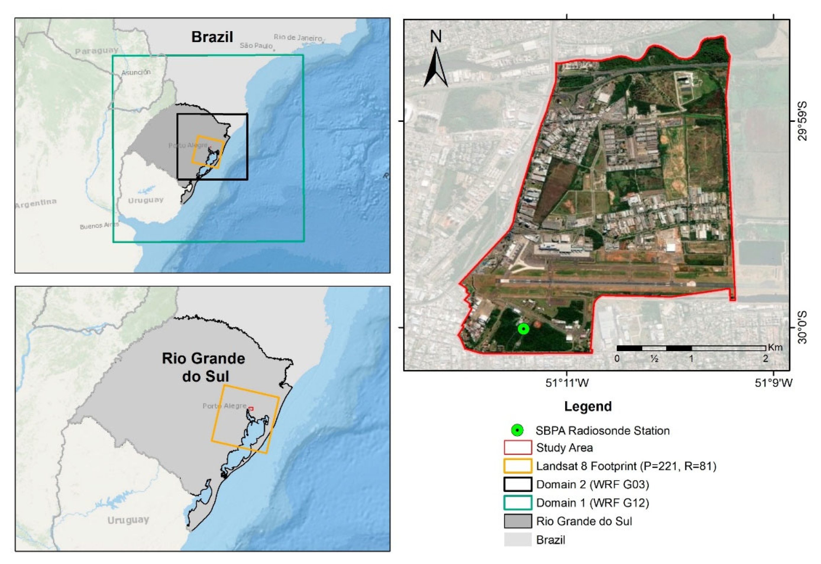
2.1. Study Area and In Situ Radiosonde Data

The Porto Alegre International Airport (SBPA), Rio Grande do Sul State, Brazil was selected as the study area. The airport includes a radiosonde station, which made this site a useful environment for studies that aimed to evaluate atmospheric profiles. The selected area covers the official limits of the Anchieta district [70], with an area of around 9.2 km2 (Figure 1). According to Köppen’s climate classification, the local climate is subtropical humid with hot summers (Cfa) [71], with a mean annual air temperature of 19.6 °C, mean annual relative humidity of 76.1%, and mean annual precipitation of 1397 mm [72].
The SBPA station is located at 30.00° S and 51.18° W, 3.0 m above mean sea level, and its identifier number is 83971. In this station, radiosondes are launched twice a day, at 00:00 and 12:00 UTC. In this study, we used the 12:00 UTC radiosonde profiles, as this is the closest time to the Landsat 8 crossing time over the study site (~13 UTC). Data were obtained from the University of Wyoming website (http://weather.uwyo.edu/upperair/sounding.html, accessed on 28 October 2021). This dataset allows the vertical structure of the atmosphere to be characterized, with profiles of air temperature, pressure, and humidity with up to 99 vertical levels. The radiosonde observations, as well as the parameters calculated from them, are considered as ground truth for the assessments in this study.

2.2. Landsat 8 Satellite Data and Case Days

The Landsat mission has been providing moderate-resolution space-based surface observations for almost 50 years. Landsat 8 is the most recent operational satellite of the series and was launched in February 2013. It carries a two-sensor payload: the Operational Land Imager (OLI), which has nine reflective (visible, near-infrared, and short-wave infrared) bands with a 30 m spatial resolution and the Thermal Infrared Sensor (TIRS) with two bands in the TIR region. The TIRS bands have a 100 m spatial resolution but it is resampled and provided at 30 m by the United States Geological Survey (USGS), to be consistent with the OLI bands [73,74].
In this study, we acquired all Landsat 8 images (Collection 1) available under daily clear-sky conditions over the study area from 2013 to 2019. This resulted in a total of 27 scenes at Path-Row 221-81 (Figure 1), with an acquisition scene center time around 13:20 UTC. The full-swath Landsat data were reduced to a subset for a 10,184-pixel region covering the study area of Figure 1. Table 1 presents the specifications of the Landsat 8 data utilized in the study, as well as the case days that henceforward will be used to refer to each dataset. Seeking to illustrate the meteorological conditions near the acquisition time, we also include in Table 1 the air temperature and the water vapor content in the atmosphere, using the precipitable water vapor (PWV) data for the entire radiosonde column measured by the SBPA station. TIRS band 10 (10.60–11.19 µm) was used for RTE-based LST retrieval (Section 2.6.2) and OLI bands 4—red (0.64–0.67 µm) and 5—near-infrared (0.85–0.88 µm) for land surface emissivity estimation (Section 2.5).

2.3. Reanalysis Data

The NCEP Climate Forecast System version 2 (CFSv2) [68] reanalysis data are produced using the NCEP Global Forecasting System (GFS) atmospheric model and the Gridpoint Statistical Interpolation (GSI) analysis system with three-dimensional variational data assimilation (3D-Var). This is arranged in grids with a horizontal resolution of 0.5° × 0.5° and in 37 vertical (pressure) levels (1000—1 mbar), with 0.205° for surface parameters. We used CFSv2 reanalysis data from the 6-hourly product as initial and boundary conditions for the WRF simulations. In addition, profiles retrieved directly from NCEP CFSv2 were included in the analysis, to assess the WRF model downscaling performance. These profiles were extracted from the grid point closest to the SBPA station.

2.4. WRF Model Configuration

The WRF model version 4.1.2 with the advanced research WRF (ARW) dynamical solver [59,75] was used to perform high-resolution numerical simulations. We configured the WRF domains with two nested grids, in one-way mode, centered at the SBPA station, with horizontal resolutions of 12 km (G12) and 3 km (G03) (4:1 parent grid ratio) (see Figure 1) and 33 sigma vertical levels with 50 hPa as the top pressure value. The time step used for the outermost domain was 72 s with a 4:1 parent ratio. Geographical static data such as land use, topography, albedo, and reflectance, were inserted into the modeling process using the land use categories of USGS.
Some atmospheric physical processes cannot be directly resolved by the numerical model and so need to be parameterized. Parameterization schemes represent the contribution of unresolved but important phenomena in terms of variables resolved at the model discrete grid [76,77,78]. The WRF model has a vast range of parameterization scheme options. The physics parameterization chosen for our simulations included: Purdue Lin microphysics parameterization [79]; the Yonsei University (YSU) Planetary Boundary Layer (PBL) scheme [80]; the Betts–Miller–Janjic (BMJ) cumulus scheme [81]; Dudhia shortwave radiation [82]; the Rapid Radiative Transfer Model (RRTM) longwave radiation option [83]; the Unified NOAH Land-Surface Model (LSM) [84]; the revised MM5 surface-layer scheme [85]. In Diaz et al. (2021) [86], some parametrization options were tested for the same SBPA area, and the set used here is based on these results and those of Santos and Nascimento (2016) [87]. The WRF configurations are summarized in Table 2 [88].
The WRF model was run using the above configurations for each of the case days in Table 1. We conducted simulations of 24 h duration starting at 00:00 UTC and the resulting profiles were extracted at 12:00 UTC for the grid point closest to the SBPA station, to match with the local radiosonde observations. Hence, the first 12 h of the simulation was considered to be spin-up time. The model output for each domain was stored every 30 min.

2.5. Land Surface Emissivity Estimation

Land surface emissivity (LSE) is one of the key parameters for retrieving LST from remote sensing data. It is a measure of the surface’s intrinsic ability to convert heat energy into radiant energy. LSE is a function of the composition, roughness, and moisture of the surface and the observation conditions [74,89,90]. Among the methods for LSE retrieval from space, those based on the normalized difference vegetation index (NDVI) are operational and are the most frequently applied, with satisfactory results [89,91,92,93,94,95,96]. Sekertekin and Bonafoni (2020a, 2020b) [74,97] examined the influence of six NDVI-based LSE models on the performance of LST retrieval. Based on their results, we opted to use the NDVI threshold method (NDVITHM) of Sobrino et al. (2008) [91]. The LSE estimation from satellites inevitably has errors and NDVI-based methods also have their limitations, especially in urban environments [98]. However, a recent study [99] reported that the use of LSE data estimated by different methods resulted in no significant variations in the LST accuracy. Nevertheless, assessing the LSE estimation is beyond the scope of this paper.
To calculate the NDVI from Landsat 8 data, the first step is to convert the digital number (DN) values of bands 4 (red) and 5 (near-infrared—NIR) to reflectances using Equation (1) [97,100]:
ρ λ = M p · Q CAL +   A p sin θ SE
where ρ λ is the reflectance of the corresponding band, MP is the multiplicative rescaling factor of the corresponding band, QCAL is the calibrated and quantized standard product of pixel values (DNs), AP is the additive rescaling factor of the corresponding band, and θ SE is the local sun elevation angle.
Then, the NDVI is obtained from Equation (2):
NDVI = ρ NIR   ρ R ρ NIR +   ρ R
where ρ NIR is the reflectance of the NIR band and ρ R is the reflectance of the red band. It is not necessary to correct the atmospheric effects in the red and NIR bands to estimate LSE [101].
From the NDVI, it is possible to calculate the fractional vegetation cover ( P V ) from Equation (3) [102]:
P V = [ NDVI   NDVI min NDVI max   NDVI min ] 2
where NDVI min = 0.2 and NDVI max = 0.5 in a global context [30,91,103]. The P V is an important factor in the LSE estimation.
The NDVITHM proposed by (Sobrino et al., 2008) [91] estimates the LSE considering three different cases as presented in Equation (4), for Landsat 8 [74]:
ε = { 0.979 0.035 ρ R 0.004 P V + 0.986 0.99 NDVI <   0.2 0.2   NDVI   0.5 NDVI >   0.5
where ε is the land surface emissivity (LSE). For NDVI < 0.2, the pixel is considered to be bare soil, and the emissivity is calculated using the reflectance of the red band. In the second case (0.2 ≤ NDVI ≤ 0.5), the pixel is considered to be composed of a mixture of bare soil and vegetation and the LSE depends on the P V value. The pixels with NDVI values higher than 0.5 are considered to be fully vegetated areas and the emissivity is assumed to be 0.99.

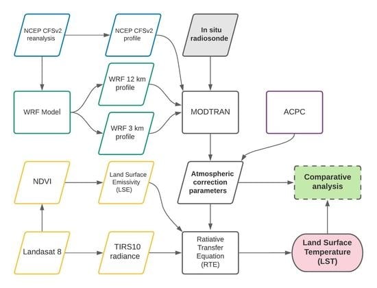
2.6. Atmospheric Correction and LST Retrieval

2.6.1. Atmospheric Parameters Calculation with MODTRAN and ACPC

MODTRAN (moderate resolution atmospheric transmission) is a commercial and widely employed atmospheric RTM developed by the U.S. Air Force and Spectral Sciences Inc. [42]. The present study used the MODTRAN4 v3r1 [104] to estimate the three atmospheric correction parameters (i.e., atmospheric transmittance, upwelling atmospheric radiance, and downwelling atmospheric radiance) in the Landsat TIR spectrum. We introduced into the MODTRAN as input, vertical profiles of pressure, air temperature, and relative humidity from: (i) SBPA radiosonde; (ii) NCEP CFSv2 reanalysis; (iii) WRF G12; (iv) WRF G03. The atmospheric parameters calculated from SBPA profiles were treated as ground truth data.
The methodology of Barsi et al. (2003) [29] was adopted to fulfill the profiles. To predict space-reaching atmospheric parameters, MODTRAN requires atmospheric profiles reaching “space”, or 100 km above sea level. Since the radiosondes and NCEP CFSv2 stretch from the surface to about 30 and 50 km, respectively, the upper atmosphere layers (to 100 km) were extracted from the MODTRAN standard atmospheres and pasted into our site-specific profiles. We used the standard mid-latitude summer profile [105] for case days in hot seasons (spring and summer) and the mid-latitude winter profile [106] for those in cold seasons (autumn and winter). The WRF-simulated profiles refined the NCEP CFSv2 profiles by increasing the number of levels in the portion of the atmosphere closest to the surface. The model was set up with the top pressure level at 50 hPa (~18 km). Thus, these profiles were completed first with the remaining levels from the reanalysis and then, starting at 50 km, with MODTRAN standard atmospheres.
This approach results in surface-to-space vertical profiles of air temperature, pressure, and water vapor. The profiles constructed for MODTRAN from the NCEP CFSv2 reanalysis count 40 (43) vertical levels in the warm (cold) seasons. Using WRF, the number of vertical levels in the filled profiles increases to 45 (48). The radiosondes describe the atmospheric profile in more detail, but the number of vertical levels varies, averaging 88 and reaching 109 in our final profiles. These completed profiles were inserted into a MODTRAN input file and then processed [27,29].
MODTRAN outputs are provided in the model’s spectral resolution, so an integration must be performed between the bounds defined by the spectral response curve of the sensor band (Equation (5)) [4]:
var   ( λ i ) = λ i , min λ i , max var   ( λ ) R s ( λ ) d λ λ i , min λ i , max R s ( λ ) d λ
where R s is the spectral response of the sensor at the center wavelength λ i of a band with a spectral window of λ i , min λ i , max and var alternatively denotes the atmospheric parameter (transmittance, upwelling, or downwelling radiance) value extracted from the MODTRAN output file, between the wavelengths λ i , min and λ i , max . In this case, the spectral response curve is from the Landsat 8 TIRS band 10 (TIRS10).
Additionally, we included in the comparative analysis the atmospheric parameters estimated by NASA’s well-established Atmospheric Correction Parameter Calculator (ACPC) web-tool [27,29]. As mentioned above, the ACPC uses NCEP reanalysis profiles (with 1° × 1° horizontal resolution and 28 vertical levels), MODTRAN code, and a suite of integration algorithms to provide the AC parameters for the particular date, time, and location inputted. The reanalysis profiles used by ACPC are to about 30 km, so they are fulfilled using MODTRAN standard atmospheres. Completed ACPC profiles have 33 vertical levels. The mid-latitude standard upper profiles varied according to the season of each case day. The option of using the atmospheric profile from the closest integer coordinate to the inputted location (SBPA station) was set.

2.6.2. Radiative Transfer Equation (RTE)-Based LST Retrieval Method

The inverse solution of the RTE [28] is a direct and a priori the most appropriate procedure for LST retrieval using a single TIR band [101]. The RTE applied to a particular TIR band/wavelength ( λ ) can be simplified and given by:
L λ sen = [ ε λ B λ ( T s ) + ( 1 ε λ ) L λ ] τ λ + L λ
where L λ sen (W·m−2·sr−1·µm−1) is the at-sensor (TOA) spectral radiance of the corresponding TIR band (in this paper, TIRS10), ε λ refers to the LSE (dimensionless), B λ (W·m−2·sr−1·µm−1) is the black body radiance, T s (Kelvin) represents the LST, L λ and L λ (W·m−2·sr−1·µm−1) refer to the downwelling and upwelling radiances, respectively, and τ λ is the atmospheric transmittance (dimensionless). Hence, the emitted radiance for a black body at a temperature T s is given by the inversion of Equation (6):
B λ ( T s ) = L λ sen L λ τ ( 1 ε λ ) L λ τ λ ε λ
where the L λ sen of Landsat 8 TIRS10 is obtained by converting the DN values ( Q CAL ) applying Equation (8) [100]:
L λ sen =   M L · Q CAL +   A L
where M L and A L are the multiplicative and additive rescaling factors of the corresponding band (TIRS10). In addition, B λ comes from Planck’s law:
B λ ( T ) = C 1 λ 5 ( e C 2 / λ T 1 )
where C 1 = 1.19104 × 10⁸ W·μm4·m−2·sr−1 and C 2 = 14,387.7 µm·K are Planck’s radiation constants. Thus, T s is calculated by inverting Planck’s law in Equation (7):
T s = C 2 λ [ ln ( C 1 λ 5 [ L λ sen L λ ε λ τ λ ( 1 ε λ ε λ ) L λ ] + 1 ) ] 1
Finally, Equation (10) can be simplified and the LST ( T s ) from Landsat 8 TIRS10 is estimated as:
LST = K 2 ln ( K 1 L λ sen L λ τ λ ( 1 ε λ ) L λ τ λ ε λ + 1 )
where K 1 and K 2 refer to calibration constants, whose values for Landsat 8 TIRS10 are 774.89 W·m−2·sr−1·µm−1 and 1321.08 K, respectively [100]. Henceforth, the spectral notation ( λ ) will be omitted, since here only a single TIR band is used.
The aforementioned procedure was applied with τ, L , and L calculated using profiles from:
  • SBPA local radiosonde;
  • NCEP CFSv2 reanalysis;
  • WRF G12;
  • WRF G03;
  • ACPC.
The LST images retrieved using the atmospheric parameters from SBPA radiosondes are considered as “ground truth”, and LST retrievals considering the other cases were compared to this, as detailed in the next section.

2.7. Metrics for Performance Evaluation

To evaluate the performance of the WRF model and other profiles we take into account the atmospheric parameters (τ, L , and L ) and LST images. The SBPA radiosondes are the available in situ observations. Hence, the AC parameters and LSTs calculated using SBPA profiles are considered our references. To perform the comparative assessment, the Pearson’s correlation coefficient (R), bias (mean error), mean absolute error (MAE), and root mean square error (RMSE) were used as statistical criteria. These metrics are widely employed to evaluate and compare models [31,107,108]. The metrics’ equations are given as follows:
R = i = 1 n ( p i   p ¯ ) ( o i   o ¯ ) i = 1 n ( p i   p ¯ ) 2 i = 1 n ( o i   o ¯ ) 2
bias = 1 n i = 1 n ( p i o i )
MAE = 1 n i = 1 n | p i o i |
RMSE = 1 n i = 1 n ( p i o i ) 2
where p i and o i are pairwise predicted and observed values, respectively, n is the number of pairs, and terms with overbars are respective mean values.
R scores range from −1 to 1, and values approaching 1 indicate stronger correlations. Bias is useful in determining if the model is underestimating (bias < 0) or overestimating (bias > 0) the observed values. MAE is the average of the absolute difference between the predictions and the observations, despite model overestimation or underestimation. It is a negatively oriented index (values closer to zero are better). RMSE is also negatively oriented. It indicates the deviation between modeled and observed values and is more sensitive to outliers as the errors are squared before summing.

3. Results and Discussion

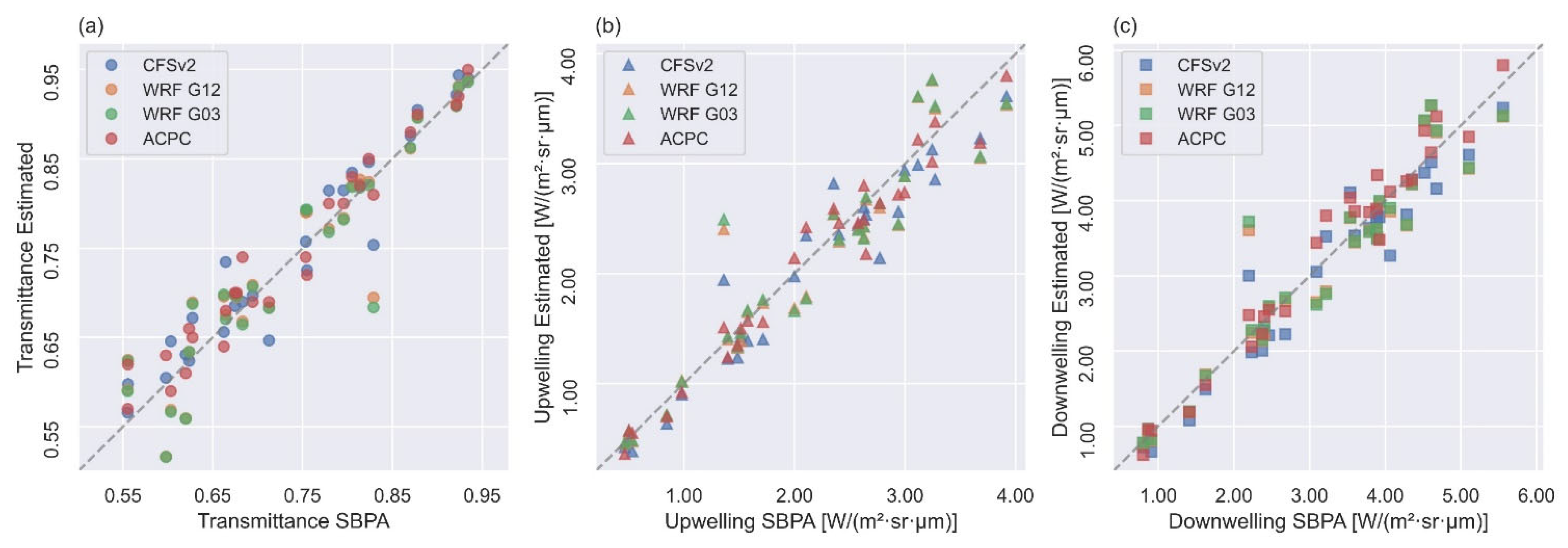
3.1. Evaluation of Atmospheric Parameters

3.1.1. Overall Results

The AC parameters (τ, L , and L ) calculated with different sources of estimated vertical profiles (CFSv2, WRF G12, WRF G03, and ACPC) were compared against those using observational SBPA radiosondes (Figure 2). In Table 3, the accuracies of atmospheric parameter estimations are presented. All the profile sources provide AC parameters with high correlation coefficients, all greater than 0.9 in relation to the reference (SBPA). The R values of ACPC are slightly better, followed by those of CFSv2. There is a general but small tendency to overestimate the transmittance values. On the other hand, the atmospheric radiances tend to be underestimated, except for ACPC downwelling. The smallest biases were from the WRF for all three parameters. The largest were from CFSv2. With respect to MAE and RMSE, the best results were from ACPC followed by CFSv2. The largest RMSE value found was 0.43 W·m−2·sr−1·µm−1 for the downwelling calculated with WRF G03 profiles.
The higher negative bias of the atmospheric radiances with NCEP CFSv2 in our findings may be due to the fact that these reanalysis profiles have the lowest level at 1000 hPa, which corresponds to around 60–250 m for the SBPA station in our case days. Therefore, the lowest layer of the atmosphere (which typically presents the largest water vapor content and warmest temperature) is neglected in these profiles. This fact was indicated by Coll et al. (2012) [32] and Meng and Cheng (2018) [20]. We tried to reduce this limitation by downscaling the CFSv2 reanalysis profiles with the WRF model. The WRF profiles bring the first level to around 1 m above the surface.
Figure 3 illustrates the performance of the AC parameters from the different profile sources via Taylor diagrams [109]. These quantify the agreement of the modeled profiles with the observational profiles in terms of graphical representations of the three statistics combined: standard deviation, root mean squared deviation (RMSD, the same as RMSE), and correlation coefficient. Figure 3 corroborates the results shown in Table 3. It indicates that ACPC obtained better results than the other profiles for all three atmospheric parameters. Next was the CFSv2 reanalysis profiles. The diagrams clearly point out that the profiles from WRF G12 and G03 had very similar accuracies. In fact, no significant statistical differences were found between the parameters from the WRF grids G12 and G03. This suggests that computation costs can be saved by using profiles from a WRF domain with coarse horizontal resolution. Despite other aims, scholars have already reported this kind of result with WRF model grids [57,110,111,112].
Our RMSE range is in agreement with the findings for reanalysis profiles in Meng and Cheng (2018) [20] for the three parameters. The authors analyzed 30,715 atmospheric profiles in 163 stations around the globe. The RMSE values of Yang et al., (2020) [40] were overall slightly lower than ours. However, their assessment only includes profiles from Europe. In Diaz et al. (2021) [85], the vertical distributions of air temperature and water vapor for the SBPA radiosondes, CFSv2 reanalysis, and WRF (G12 and G03) profiles were compared. The evaluation of the profiles themselves showed that both CFSv2 and WRF models skillfully represent the vertical profiles of temperature and water vapor. Nevertheless, the statistical metrics indicated that increasing the horizontal resolution did not significantly improve the quality of the simulated atmospheric profile. This is in line with the above results for the atmospheric parameters comparison.

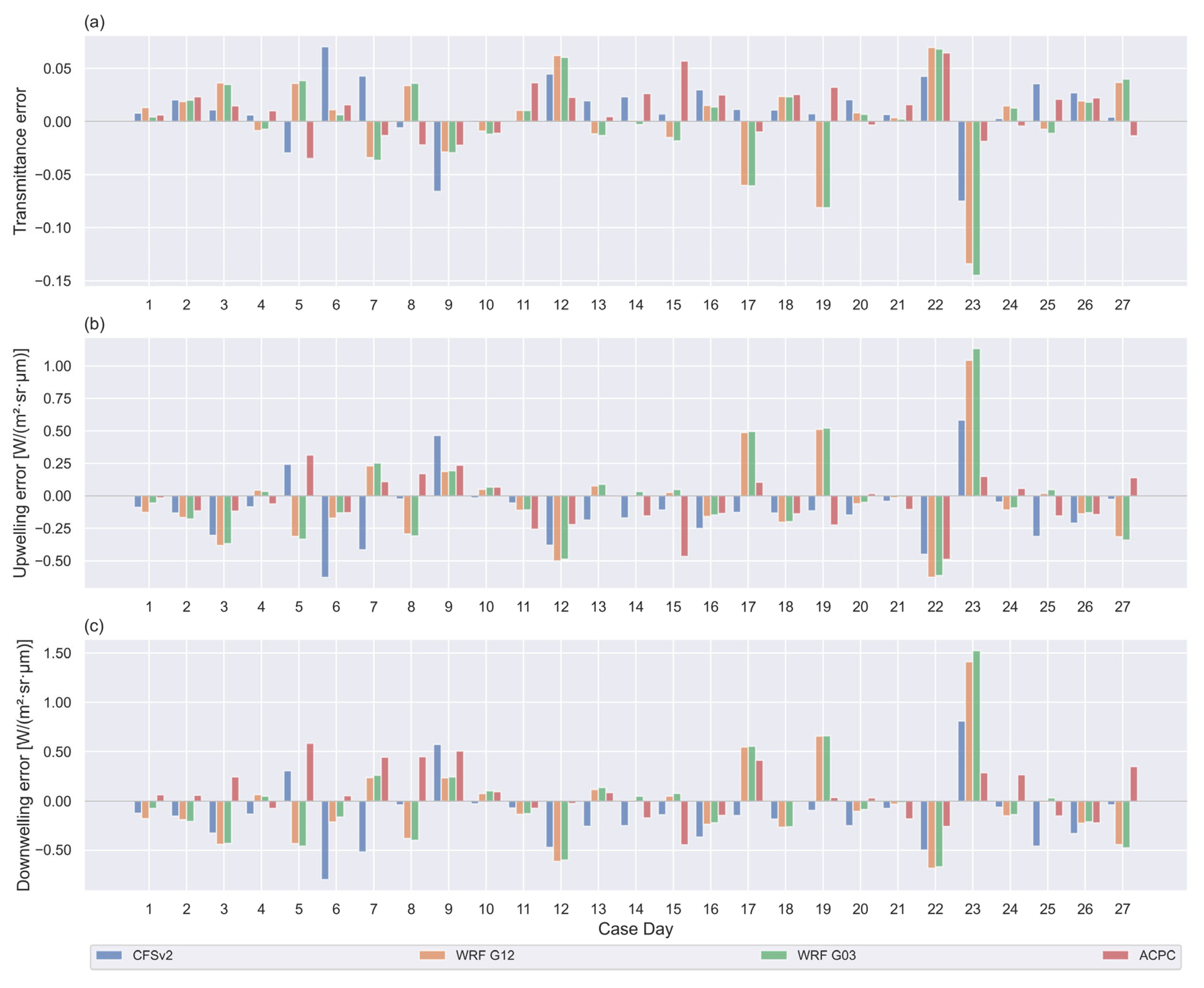
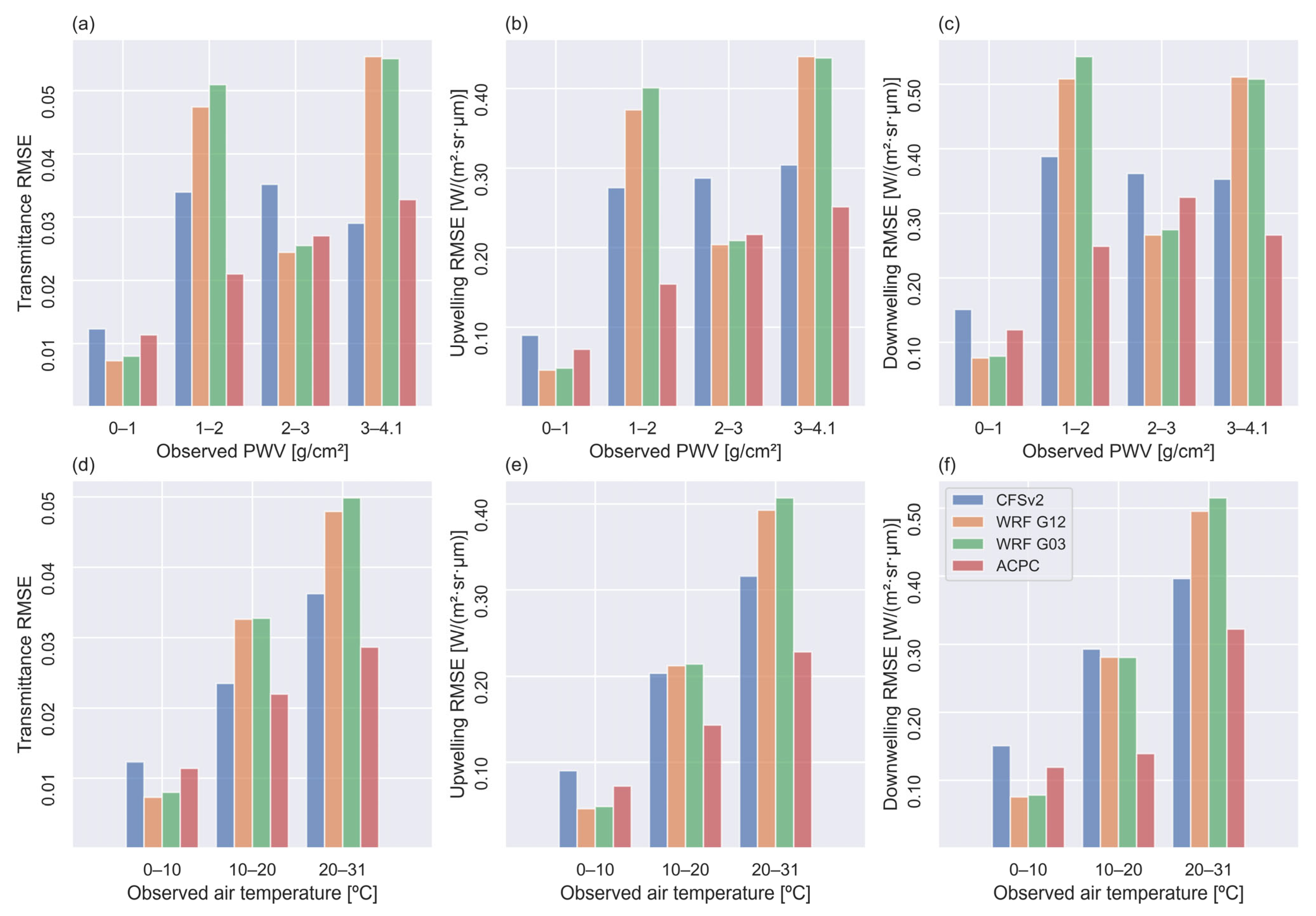
3.1.2. Analysis by Meteorological Conditions

The errors in the estimation of atmospheric parameters for each case day are shown in Figure 4. This shows that, despite the fact that ACPC presented the best overall metrics, none of the profile sources performed best in all cases. For instance, in eight of the case days, one of the WRF profiles had the best results in calculating the downwelling radiance. For case day 23, the WRF model plainly produced the largest errors, whereas for case days such as day 26, the model successfully reduced the largest error in the driving reanalysis data. Therefore, it is pertinent to assess the dependence of the performances of different profile sources on the meteorological conditions.
Figure 5 shows the RMSE values of the AC parameters calculated taking into account specific ranges of precipitable water vapor (PWV) for the entire atmospheric column (measured by SBPA radiosondes) and air temperature observed at the SBPA station (Table 1). The WRF model performs better under dry and cold conditions. It outperforms the other profile sources in the range of 2–3 g/cm2 PWV. Under almost all moisture and temperature conditions, the ACPC profiles presented better results than the NCEP CFSv2 profiles. All the different profiles presented minor errors in situations of the lowest water vapor and air temperature. However, it is important to mention that the number of case days under these conditions was less than for the other ranges. This is consistent with the research of Meng and Cheng (2018) [20], where it was noted that the best global RMSEs were for profiles with a water vapor content lower than 1 g/cm2. Furthermore, they indicated that the largest RMSEs occurred when the water vapor was between 3 and 4 g/cm2. With respect to the air temperature, our results suggest that errors in estimating the atmospheric parameters are higher on warmer days.

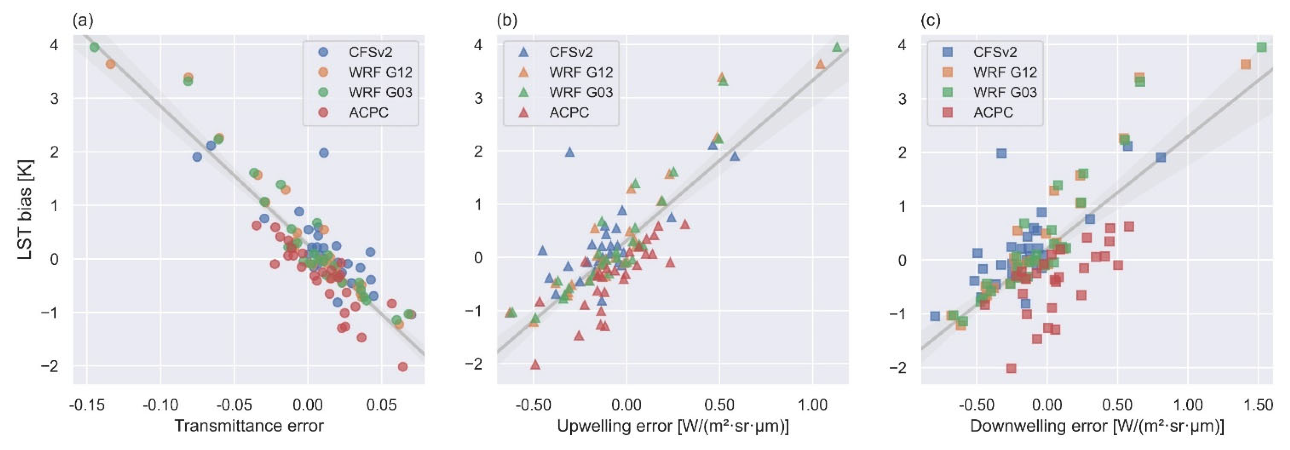
3.2. Application to RTE-Based LST Retrieval

To further assess the different atmospheric profiles, the LSTs retrieved by RTE inversion with atmospheric parameters, Landsat 8 TIRS10 radiance, and NDVITHM emissivity were compared with each other. Once more, the LST images that used SBPA profiles were assumed as reference data. Except for the atmospheric parameters calculated from the different profile sources, the other variables in Equation (11) were the same for each pixel of the scenes. Therefore, the differences between LST values that were retrieved with SBPA profiles and those from other sources were due to the discrepancies among the profiles [40]. Figure 6 illustrates an example (case day 25) of the LST spatial distribution in the study area. Note that the hottest pixels are over the airstrip and adjacent buildings of the airport.
Histograms of LST errors for all the 10,184 pixels in the study area of the 27 case days are shown in Figure 7. These represent the frequency distribution of the errors in the retrieval of LST using the different atmospheric profile sources. For all profiles, more than 50% of the errors are in the range of ±1 K. Yang et al. (2020) [40] also found the most LST differences in this range, using different reanalysis and satellite-derived profiles. The histograms in Figure 7b,c indicate that WRF profiles tend to overestimate the LST, whereas ACPC tends to underestimate it (Figure 7d). Using WRF profiles, LST errors can reach to more than 4 K, although only in a very small number of cases. For ACPC and both WRF grids, the error range that occurs most often is between 0 and −1 K. The distribution of CFSv2 LST errors is more symmetrical than in the other profiles.
Table 4 summarizes the metrics of the LST retrieval comparative analysis. Overall, the LST values of the four profile sources analyzed in this study were found to be in good agreement with the reference. All of them showed a very strong correlation and relatively low bias, MAE, and RMSE values. CFSv2, WRF G12, and WRF G03 presented an average positive bias and ACPC a negative bias. This corresponds with the histogram analysis in Figure 7. The mean error criteria (MAE and RMSE) indicate that the profiles with the best performance in the AC- and RTE-based LST retrieval are, in descending order: CFSv2, ACPC, WRF G12, and WRF G03. The differences between CFSv2 and ACPC overall MAE and RMSE values were very small, and similarly for WRF G12 and G03.
Comparing these results with previous studies that evaluated the application of different atmospheric profiles for LST retrieval, Meng and Cheng (2018) [20] reported overall LST RMSE values higher than ours for eight different reanalysis profile sources analyzed around the globe. All their eight average RMSEs were larger than 1 K. The authors mention that ERA-Interim and MERRA (6 h product) showed the lowest RMSEs, at 1.09 K and 1.07 K respectively. They also indicated an average tendency to overestimate the LST, except for JRA-55. In Yang et al. (2020) [39], RMSEs were smaller than 0.6 K using profiles from ERA-Interim, MERRA2, NCEP GFS, and NCEP FNL, over Europe. Their worst accuracy (RMSE of 1 K) was obtained using MOD07 satellite-based profiles. Retrieving LST from three MODIS thermal bands, Pérez-Planells et al. (2015) [33] showed RMSEs between 0.6 and 0.9 K using ACPC/NCEP and between 1.3 and 3 K for MOD07 profiles, depending on the band and the altitude of the study sites in Spain.
Figure 8 displays the distribution of LST bias and RMSE among the case days. Figure 8a evidences the ACPC and WRF settings’ average tendency to under and overestimate the LST, respectively. We found better RMSE values using CFSv2 in 11 of the 27 case days, and in 8 using ACPC. However, the metrics of mean errors are greater for WRF profiles, as in 11 case days the model improves the results of the reanalysis. Furthermore, the finer grid (G03) succeeded in downscaling the G12 11 times. In fact, the largest errors were achieved when using the WRF model (e.g., for case days 23, 19, and 17), contributing to the higher overall RMSE values. In general, the days with larger errors in atmospheric parameters (Figure 4) were the days with larger LST RMSEs, as in case day 23. Conversely, for case day 22, the errors in atmospheric parameters using ACPC were less than those using WRF profiles, but the highest LST RMSE on this day was with ACPC. Jiménez-Muñoz et al. (2010) [24] suggest that cases like this may be explained by compensation among the AC parameter errors, for instance, a significant positive difference in transmittance and significant but negative differences in the atmospheric radiances. Figure 9 shows how errors in the atmospheric parameters propagate to the retrieved LST. The sensitivity analysis of Sekertekin and Bonafoni (2020) [74] reported that an uncertainty of ±0.01 in atmospheric transmittance had an impact of ±0.97 K on RTE-based LST retrieval. For upwelling and downwelling, uncertainties of ±10% led to ±1.82 K and ±0.07 K errors in LST, respectively. Rosas et al. (2017) [21] mentioned that an introduced uncertainty of 20% in the relative humidity profile could result in LST errors as large as 1.5 K in arid environments.
In summary, the attempt at downscaling the horizontal resolution of reanalysis data from 0.5° (~56 km) to 12 km and so to 3 km, aiming to reduce errors in the calculation of atmospheric parameters and hence in LST retrieval, did not perform as theoretically expected. Using WRF simulations, we improved the vertical resolution in the lowest atmospheric levels. However, no significant improvement was found in the AC using the WRF profiles. In some cases, using a finer grid resolution profile resulted in even greater differences in atmospheric parameters and LST estimation. Rosas et al. (2017) [21] reported that the higher vertical resolution of NCEP and ECMWF profiles in their study did not seem to play a significant role in the atmospheric correction. Even if data with higher resolution naturally tend to represent the atmospheric parameters better, it is not a strictly direct relationship [20,40]. Furthermore, the ACPC, which uses profiles with 1° × 1° (~111 km) horizontal resolution, showed good results. Although these profiles have a coarser horizontal resolution, previous studies have found satisfactory results using the ACPC, even surpassing other methods [24,31,46,93,113,114,115,116,117]. It is important to note that in this study the WRF profiles were extracted at 12 UTC to match the available radiosonde data. Nevertheless, the extraction could be set for the exact time of the satellite overpass. In the ACPC, and in general for reanalysis profiles, this time synchronization is achieved through linear interpolation, which may not be the most appropriate strategy for sampling weather fronts and diurnal heating cycles [20,27,29].

4. Conclusions

Vertical atmospheric profiles are key inputs in the atmospheric correction for estimating LST using the RTE inversion single-channel approach. This study evaluated the use of the WRF numerical model to simulate high-resolution profiles, improving horizontal, temporal, and vertical resolutions of NCEP CFSv2 reanalysis data. The profiles were incorporated into the MODTRAN RTM to compute the atmospheric correction parameters, which were then applied in the RTE to retrieve LST values from Landsat 8 TIRS10 data. We included in the comparison analysis the widely applied ACPC web-tool. The assessment took into account 27 clear-sky Landsat 8 scenes over a radiosonde station in Southern Brazil.
The obtained results showed that for the three atmospheric parameters (atmospheric transmittance, upwelling radiance, and downwelling radiance) the ACPC provided parameters in better agreement with those calculated using the radiosondes. The second-lowest uncertainties occurred when using CFSv2 profiles. No significant statistical differences were found between the parameters from the two WRF grids. None of the profile sources outperformed the others in all case days analyzed. The overall metrics of the WRF profiles were influenced by some cases with large errors. In general, the assessed profile sources better represented the atmosphere in dry and cold conditions. With respect to the retrieved LST values, using those calculated with the SBPA profile as reference, CFSv2 had the best results. With an RMSE of 0.55 K, it was slightly more accurate than ACPC (RMSE of 0.56 K). WRF G12 and G03 showed RMSE values of 0.79 and 0.82 K, respectively. Both WRF grids and CFSv2 generated a positive LST bias, while ACPC generated a negative bias. On balance, all the profile sources presented relatively good results in estimating the LST.
From the above findings, we conclude the following.
  • Our main conclusion is that there is no special need to increase the horizontal resolution of reanalysis profiles aiming at general RTE-based LST retrieval. We recommend the use of NCEP CFSv2 profiles for these applications.
  • The results reinforce the validity and feasibility of ACPC, which is free of charge.
  • Even though the overall statistical metrics for WRF profiles were inferior, their results were satisfactory for the estimation of both atmospheric parameters and LST values.
Despite the fact that some studies used the WRF model to simulate the skin temperature [118,119], to the best of our knowledge, this paper is the first attempt to apply the WRF model to aid the atmospheric correction of thermal remote sensing data. Its use showed potential, and our findings encourage further validations. Our study adds to the background of studies combing TIR satellite images and high-resolution NWP models.
Finally, in spite of the discoveries in this study, some limitations to be considered in future work are worth mentioning. There were no in situ LST data available to perform validation of the retrieved LST. The uncertainties in the SBPA radiosonde profiles were not analyzed; they were directly assumed as reference data. The study results refer to one area only, and therefore additional research is currently ongoing to extrapolate the conclusions to other environments.

Author Contributions

Conceptualization, L.R.D., D.C.S. and S.B.A.R.; methodology, L.R.D., D.C.S., P.S.K. and S.B.A.R.; software, L.R.D., D.C.S., P.S.K. and S.T.L.d.C.; validation, L.R.D. and D.C.S.; investigation, L.R.D., D.C.S., P.S.K., N.S.d.R., S.T.L.d.C. and E.A.K.; resources, S.B.A.R.; data curation, L.R.D., D.C.S. and E.A.K.; writing—original draft preparation, L.R.D.; writing—review and editing, L.R.D., D.C.S., P.S.K., N.S.d.R. and S.B.A.R.; supervision, S.B.A.R.; project administration, S.B.A.R.; funding acquisition, S.B.A.R. All authors have read and agreed to the published version of the manuscript.

Funding

This study was financed in part by the Coordenação de Aperfeiçoamento de Pessoal de Nível Superior—Brazil (CAPES), finance code 001, grant number 88882.438973/2019-01.

Data Availability Statement

The Landsat 8 data are courtesy of the US Geological Survey Earth Resources Observation and Science Center. The CFSv2 reanalysis data are provided by the National Centers for Environmental Prediction (NCEP), available at the Research Data Archive (RDA)—National Center for Atmospheric Research (NCAR). The radiosonde observations were obtained from the University of Wyoming website.

Acknowledgments

The anonymous reviewers are thanked for their valuable contributions. We are also grateful to Luis Morales-Salinas (University of Chile) and Dražen Skokovic (University of Valencia) for their support regarding the MODTRAN model.

Conflicts of Interest

The authors declare no conflict of interest. The funders had no role in the design of the study, in the collection, analyses, or interpretation of data, in the writing of the manuscript, or in the decision to publish the results.

References

  1. Cao, B.; Liu, Q.; Du, Y.; Roujean, J.L.; Gastellu-Etchegorry, J.P.; Trigo, I.F.; Zhan, W.; Yu, Y.; Cheng, J.; Jacob, F.; et al. A Review of Earth Surface Thermal Radiation Directionality Observing and Modeling: Historical Development, Current Status and Perspectives. Remote Sens. Environ. 2019, 232, 111304. [Google Scholar] [CrossRef]
  2. WMO. The Global Observing System for Climate: Implementation Needs; World Meteorological Organization (WMO): Geneva, Switzerland, 2016; Volume 200. [Google Scholar]
  3. Anderson, M.C.; Norman, J.M.; Kustas, W.P.; Houborg, R.; Starks, P.J.; Agam, N. A Thermal-Based Remote Sensing Technique for Routine Mapping of Land-Surface Carbon, Water and Energy Fluxes from Field to Regional Scales. Remote Sens. Environ. 2008, 112, 4227–4241. [Google Scholar] [CrossRef]
  4. Tardy, B.; Rivalland, V.; Huc, M.; Hagolle, O.; Marcq, S.; Boulet, G. A Software Tool for Atmospheric Correction and Surface Temperature Estimation of Landsat Infrared Thermal Data. Remote Sens. 2016, 8, 696. [Google Scholar] [CrossRef] [Green Version]
  5. Wu, P.; Yin, Z.; Zeng, C.; Duan, S.-B.; Gottsche, F.-M.; Li, X.; Ma, X.; Yang, H.; Shen, H. Spatially Continuous and High-Resolution Land Surface Temperature Product Generation: A Review of Reconstruction and Spatiotemporal Fusion Techniques. IEEE Geosci. Remote Sens. Mag. 2021, 9, 112–137. [Google Scholar] [CrossRef]
  6. Sobrino, J.A.; Del Frate, F.; Drusch, M.; Jiménez-Muñoz, J.C.; Manunta, P.; Regan, A. Review of Thermal Infrared Applications and Requirements for Future High-Resolution Sensors. IEEE Trans. Geosci. Remote Sens. 2016, 54, 2963–2972. [Google Scholar] [CrossRef]
  7. Montaner-Fernández, D.; Morales-Salinas, L.; Rodriguez, J.S.; Cárdenas-Jirón, L.; Huete, A.; Fuentes-Jaque, G.; Pérez-Martínez, W.; Cabezas, J. Spatio-Temporal Variation of the Urban Heat Island in Santiago, Chile during Summers 2005–2017. Remote Sens. 2020, 12, 3345. [Google Scholar] [CrossRef]
  8. Candy, B.; Saunders, R.W.; Ghent, D.; Bulgin, C.E. The Impact of Satellite-Derived Land Surface Temperatures on Numerical Weather Prediction Analyses and Forecasts. J. Geophys. Res. Atmos. 2017, 122, 9783–9802. [Google Scholar] [CrossRef] [Green Version]
  9. Hu, X.; Ren, H.; Tansey, K.; Zheng, Y.; Ghent, D.; Liu, X.; Yan, L. Agricultural Drought Monitoring Using European Space Agency Sentinel 3A Land Surface Temperature and Normalized Difference Vegetation Index Imageries. Agric. For. Meteorol. 2019, 279, 107707. [Google Scholar] [CrossRef]
  10. Jiménez-Muñoz, J.C.; Mattar, C.; Sobrino, J.A.; Malhi, Y. Digital Thermal Monitoring of the Amazon Forest: An Intercomparison of Satellite and Reanalysis Products. Int. J. Digit. Earth 2016, 9, 477–498. [Google Scholar] [CrossRef]
  11. Magarreiro, C.; Gouveia, C.; Barroso, C.; Trigo, I. Modelling of Wine Production Using Land Surface Temperature and FAPAR—The Case of the Douro Wine Region. Remote Sens. 2019, 11, 604. [Google Scholar] [CrossRef] [Green Version]
  12. Pavlidou, E.; van der Meijde, M.; van der Werff, H.; Hecker, C. Time Series Analysis of Land Surface Temperatures in 20 Earthquake Casesworldwide. Remote Sens. 2019, 11, 61. [Google Scholar] [CrossRef] [Green Version]
  13. Gemitzi, A.; Dalampakis, P.; Falalakis, G. International Journal of Applied Earth Observations and Geoinformation Detecting Geothermal Anomalies Using Landsat 8 Thermal Infrared Remotely Sensed Data. Int. J. Appl. Earth Obs. Geoinf. 2021, 96, 102283. [Google Scholar] [CrossRef]
  14. da Rocha, N.S.; Käfer, P.S.; Skokovic, D.; Veeck, G.; Diaz, L.R.; Kaiser, E.A.; Carvalho, C.M.; Cruz, R.C.; Sobrino, J.A.; Roberti, D.R.; et al. The Influence of Land Surface Temperature in Evapotranspiration Estimated by the S-SEBI Model. Atmosphere 2020, 11, 1059. [Google Scholar] [CrossRef]
  15. Anderson, M.C.; Yang, Y.; Xue, J.; Knipper, K.R.; Yang, Y.; Gao, F.; Hain, C.R.; Kustas, W.P.; Cawse-Nicholson, K.; Hulley, G.; et al. Interoperability of ECOSTRESS and Landsat for Mapping Evapotranspiration Time Series at Sub-Field Scales. Remote Sens. Environ. 2021, 252, 112189. [Google Scholar] [CrossRef]
  16. Maffei, C.; Alfieri, S.M.; Menenti, M. Relating Spatiotemporal Patterns of Forest Fires Burned Area and Duration to Diurnal Land Surface Temperature Anomalies. Remote Sens. 2018, 10, 1777. [Google Scholar] [CrossRef] [Green Version]
  17. Singh, N.; Chatterjee, R.S.; Kumar, D.; Panigrahi, D.C.; Mujawdiya, R. Retrieval of Precise Land Surface Temperature from ASTER Night-Time Thermal Infrared Data by Split Window Algorithm for Improved Coal Fire Detection in Jharia Coalfield, India. Geocarto Int. 2020, 1–18. [Google Scholar] [CrossRef]
  18. Anderson, M.C.; Allen, R.G.; Morse, A.; Kustas, W.P. Use of Landsat Thermal Imagery in Monitoring Evapotranspiration and Managing Water Resources. Remote Sens. Environ. 2012, 122, 50–65. [Google Scholar] [CrossRef]
  19. Tavares, M.H.; Cunha, A.H.F.; Motta-Marques, D.; Ruhoff, A.L.; Fragoso, C.R.; Munar, A.M.; Bonnet, M.P. Derivation of Consistent, Continuous Daily River Temperature Data Series by Combining Remote Sensing and Water Temperature Models. Remote Sens. Environ. 2020, 241, 111721. [Google Scholar] [CrossRef]
  20. Meng, X.; Cheng, J. Evaluating Eight Global Reanalysis Products for Atmospheric Correction of Thermal Infrared Sensor—Application to Landsat 8 TIRS10 Data. Remote Sens. 2018, 10, 474. [Google Scholar] [CrossRef] [Green Version]
  21. Rosas, J.; Houborg, R.; McCabe, M.F. Sensitivity of Landsat 8 Surface Temperature Estimates to Atmospheric Profile Data: A Study Using MODTRAN in Dryland Irrigated Systems. Remote Sens. 2017, 9, 988. [Google Scholar] [CrossRef] [Green Version]
  22. Cristóbal, J.; Jiménez-Muñoz, J.; Prakash, A.; Mattar, C.; Skoković, D.; Sobrino, J. An Improved Single-Channel Method to Retrieve Land Surface Temperature from the Landsat-8 Thermal Band. Remote Sens. 2018, 10, 431. [Google Scholar] [CrossRef] [Green Version]
  23. Li, Z.-L.; Tang, B.-H.; Wu, H.; Ren, H.; Yan, G.; Wan, Z.; Trigo, I.F.; Sobrino, J.A. Satellite-Derived Land Surface Temperature: Current Status and Perspectives. Remote Sens. Environ. 2013, 131, 14–37. [Google Scholar] [CrossRef] [Green Version]
  24. Jiménez-Muñoz, J.C.; Sobrino, J.A.; Mattar, C.; Franch, B. Atmospheric Correction of Optical Imagery from MODIS and Reanalysis Atmospheric Products. Remote Sens. Environ. 2010, 114, 2195–2210. [Google Scholar] [CrossRef]
  25. Tang, H.; Li, Z.-L. Quantitative Remote Sensing in Thermal Infrared; Springer Remote Sensing/Photogrammetry; Springer: Berlin/Heidelberg, Germany, 2014; ISBN 978-3-642-42026-9. [Google Scholar]
  26. Galve, J.M.; Sánchez, J.M.; Coll, C.; Villodre, J. A New Single-Band Pixel-by-Pixel Atmospheric Correction Method to Improve the Accuracy in Remote Sensing Estimates of LST. Application to Landsat 7-ETM+. Remote Sens. 2018, 10, 826. [Google Scholar] [CrossRef] [Green Version]
  27. Barsi, J.A.; Schott, J.R.; Palluconi, F.D.; Hook, S.J. Validation of a Web-Based Atmospheric Correction Tool for Single Thermal Band Instruments. In Proceedings of the Earth Observing Systems X, San Diego, CA, USA, 18 August 2005; Volume 5882, p. 58820E. [Google Scholar]
  28. Price, J.C. Estimating Surface Temperatures from Satellite Thermal Infrared Data—A Simple Formulation for the Atmospheric Effect. Remote Sens. Environ. 1983, 13, 353–361. [Google Scholar] [CrossRef]
  29. Barsi, J.A.; Barker, J.L.; Schott, J.R. An Atmospheric Correction Parameter Calculator for a Single Thermal Band Earth-Sensing Instrument. In Proceedings of the IGARSS 2003 IEEE International Geoscience and Remote Sensing Symposium, Toulouse, France, 21–25 July 2003; Volume 5, pp. 3014–3016. [Google Scholar]
  30. Sobrino, J.A.; Jiménez-Muñoz, J.C.; Paolini, L. Land Surface Temperature Retrieval from LANDSAT TM 5. Remote Sens. Environ. 2004, 90, 434–440. [Google Scholar] [CrossRef]
  31. Sekertekin, A. Validation of Physical Radiative Transfer Equation-Based Land Surface Temperature Using Landsat 8 Satellite Imagery and SURFRAD in-Situ Measurements. J. Atmos. Sol.-Terr. Phys. 2019, 196, 105161. [Google Scholar] [CrossRef]
  32. Coll, C.; Caselles, V.; Valor, E.; Niclòs, R. Comparison between Different Sources of Atmospheric Profiles for Land Surface Temperature Retrieval from Single Channel Thermal Infrared Data. Remote Sens. Environ. 2012, 117, 199–210. [Google Scholar] [CrossRef]
  33. Pérez-Planells, L.; García-Santos, V.; Caselles, V. Comparing Different Profiles to Characterize the Atmosphere for Three MODIS TIR Bands. Atmos. Res. 2015, 161–162, 108–115. [Google Scholar] [CrossRef] [Green Version]
  34. Mira, M.; Olioso, A.; Rivalland, V.; Courault, D.; Marloie, O.; Guillevic, P. Quantifying Uncertainties in Land Surface Temperature Due to Atmospheric Correction: Application to Landsat-7 Data over a Mediterranean Agricultural Region. In Proceedings of the 2014 IEEE Geoscience and Remote Sensing Symposium, IEEE, Quebec City, QC, Canada, 13–18 July 2014; pp. 2375–2378. [Google Scholar]
  35. Coll, C.; Caselles, V.; Galve, J.M.; Valor, E.; Niclòs, R.; Sánchez, J.M.; Rivas, R. Ground Measurements for the Validation of Land Surface Temperatures Derived from AATSR and MODIS Data. Remote Sens. Environ. 2005, 97, 288–300. [Google Scholar] [CrossRef]
  36. Mattar, C.; Durán-Alarcón, C.; Jiménez-Muñoz, J.C.; Santamaría-Artigas, A.; Olivera-Guerra, L.; Sobrino, J.A. Global Atmospheric Profiles from Reanalysis Information (GAPRI): A New Database for Earth Surface Temperature Retrieval. Int. J. Remote Sens. 2015, 36, 5045–5060. [Google Scholar] [CrossRef]
  37. Duan, S.-B.; Li, Z.-L.; Wang, C.; Zhang, S.; Tang, B.-H.; Leng, P.; Gao, M.-F. Land-Surface Temperature Retrieval from Landsat 8 Single-Channel Thermal Infrared Data in Combination with NCEP Reanalysis Data and ASTER GED Product. Int. J. Remote Sens. 2018, 40, 1763–1778. [Google Scholar] [CrossRef]
  38. Vanhellemont, Q. Automated Water Surface Temperature Retrieval from Landsat 8/TIRS. Remote Sens. Environ. 2020, 237, 111518. [Google Scholar] [CrossRef]
  39. Malakar, N.K.; Hulley, G.C.; Hook, S.J.; Laraby, K.; Cook, M.; Schott, J.R. An Operational Land Surface Temperature Product for Landsat Thermal Data: Methodology and Validation. IEEE Trans. Geosci. Remote Sens. 2018, 56, 5717–5735. [Google Scholar] [CrossRef]
  40. Yang, J.; Duan, S.B.; Zhang, X.; Wu, P.; Huang, C.; Leng, P.; Gao, M. Evaluation of Seven Atmospheric Profiles from Reanalysis and Satellite-Derived Products: Implication for Single-Channel Land Surface Temperature Retrieval. Remote Sens. 2020, 12, 791. [Google Scholar] [CrossRef] [Green Version]
  41. Alghamdi, A.S. Evaluation of Four Reanalysis Datasets against Radiosonde over Southwest Asia. Atmosphere 2020, 11, 402. [Google Scholar] [CrossRef] [Green Version]
  42. Berk, A.; Conforti, P.; Kennett, R.; Perkins, T.; Hawes, F.; van den Bosch, J. MODTRAN6: A Major Upgrade of the MODTRAN Radiative Transfer Code. In Proceedings of the Workshop on Hyperspectral Image and Signal Processing, Evolution in Remote Sensing, Lausanne, Switzerland, 13 June 2014; Volume 2014, p. 90880H. [Google Scholar]
  43. Kalnay, E.; Kanamitsu, M.; Kistler, R.; Collins, W.; Deaven, D.; Gandin, L.; Iredell, M.; Saha, S.; White, G.; Woollen, J.; et al. The NCEP/NCAR 40-Year Reanalysis Project. Bull. Am. Meteorol. Soc. 1996, 77, 437–471. [Google Scholar] [CrossRef] [Green Version]
  44. National Centers for Environmental Prediction National Weather Service NOAA. U.S. Department of Commerce NCEP FNL Operational Model Global Tropospheric Analyses, Continuing from July 1999; National Centers for Environmental Prediction National Weather Service NOAA: College Park, MD, USA, 2000. [CrossRef]
  45. Borbas, E.; Menzel, P. MODIS Atmosphere L2 Atmosphere Profile Product; NASA MODIS Adaptive Processing System; Goddard Space Flight Center: Greenbelt, MD, USA, 2017.
  46. Skokovic, D.; Sobrino, J.A.; Jimenez-Munoz, J.C. Vicarious Calibration of the Landsat 7 Thermal Infrared Band and LST Algorithm Validation of the ETM+ Instrument Using Three Global Atmospheric Profiles. IEEE Trans. Geosci. Remote Sens. 2017, 55, 1804–1811. [Google Scholar] [CrossRef]
  47. Li, H.; Liu, Q.; Du, Y.; Jiang, J.; Wang, H. Evaluation of the NCEP and MODIS Atmospheric Products for Single Channel Land Surface Temperature Retrieval with Ground Measurements: A Case Study of HJ-1B IRS Data. IEEE J. Sel. Top. Appl. Earth Obs. Remote Sens. 2013, 6, 1399–1408. [Google Scholar] [CrossRef]
  48. Aumann, H.H.; Chahine, M.T.; Gautier, C.; Goldberg, M.D.; Kalnay, E.; McMillin, L.M.; Revercomb, H.; Rosenkranz, P.W.; Smith, W.L.; Staelin, D.H.; et al. AIRS/AMSU/HSB on the Aqua Mission: Design, Science Objectives, Data Products, and Processing Systems. IEEE Trans. Geosci. Remote Sens. 2003, 41, 253–264. [Google Scholar] [CrossRef] [Green Version]
  49. Dee, D.P.; Uppala, S.M.; Simmons, A.J.; Berrisford, P.; Poli, P.; Kobayashi, S.; Andrae, U.; Balmaseda, M.A.; Balsamo, G.; Bauer, P.; et al. The ERA-Interim Reanalysis: Configuration and Performance of the Data Assimilation System. Q. J. R. Meteorol. Soc. 2011, 137, 553–597. [Google Scholar] [CrossRef]
  50. Rienecker, M.M.; Suarez, M.J.; Gelaro, R.; Todling, R.; Bacmeister, J.; Liu, E.; Bosilovich, M.G.; Schubert, S.D.; Takacs, L.; Kim, G.K.; et al. MERRA: NASA’s Modern-Era Retrospective Analysis for Research and Applications. J. Clim. 2011, 24, 3624–3648. [Google Scholar] [CrossRef]
  51. Kanamitsu, M.; Ebisuzaki, W.; Woollen, J.; Yang, S.K.; Hnilo, J.J.; Fiorino, M.; Potter, G.L. NCEP-DOE AMIP-II Reanalysis (R-2). Bull. Am. Meteorol. Soc. 2002, 83, 1631–1644. [Google Scholar] [CrossRef]
  52. Kobayashi, S.; Ota, Y.; Harada, Y.; Ebita, A.; Moriya, M.; Onoda, H.; Onogi, K.; Kamahori, H.; Kobayashi, C.; Endo, H.; et al. The JRA-55 Reanalysis: General Specifications and Basic Characteristics. J. Meteorol. Soc. Japan. Ser. II 2015, 93, 5–48. [Google Scholar] [CrossRef] [Green Version]
  53. Chen, B.; Liu, Z. Global Water Vapor Variability and Trend from the Latest 36 Year (1979 to 2014) Data of ECMWF and NCEP Reanalyses, Radiosonde, GPS, and Microwave Satellite. J. Geophys. Res. Atmos. 2016, 121, 11442–11462. [Google Scholar] [CrossRef]
  54. Chen, G.; Iwasaki, T.; Qin, H.; Sha, W. Evaluation of the Warm-Season Diurnal Variability over East Asia in Recent Reanalyses JRA-55, ERA-Interim, NCEP CFSR, and NASA MERRA. J. Clim. 2014, 27, 5517–5537. [Google Scholar] [CrossRef]
  55. Tonooka, H. An Atmospheric Correction Algorithm for Thermal Infrared Multispectral Data over Land-a Water-Vapor Scaling Method. IEEE Trans. Geosci. Remote Sens. 2001, 39, 682–692. [Google Scholar] [CrossRef]
  56. Wee, T.K.; Kuo, Y.H.; Lee, D.K.; Liu, Z.; Wang, W.; Chen, S.Y. Two Overlooked Biases of the Advanced Research Wrf (Arw) Model in Geopotential Height and Temperature. Mon. Weather Rev. 2012, 140, 3907–3918. [Google Scholar] [CrossRef]
  57. Hassanli, H.; Rahimzadegan, M. Investigating Extracted Total Precipitable Water Vapor from Weather Research and Forecasting (WRF) Model and MODIS Measurements. J. Atmos. Sol. -Terr. Phys. 2019, 193, 105060. [Google Scholar] [CrossRef]
  58. Lee, H.; Won, J.S.; Park, W. An Atmospheric Correction Using High Resolution Numericalweather Prediction Models for Satellite-Borne Single-Channel Mid-Wavelength and Thermal Infrared Imaging Sensors. Remote Sens. 2020, 12, 853. [Google Scholar] [CrossRef] [Green Version]
  59. Skamarock, W.C.; Klemp, J.B.; Dudhia, J.; Gill, D.O.; Zhiquan, L.; Berner, J.; Wang, W.; Powers, J.G.; Duda, M.G.; Barker, D.M.; et al. A Description of the Advanced Research WRF Model Version 4; National Center for Atmospheric Research: Boulder, CO, USA, 2019. [Google Scholar]
  60. Powers, J.G.; Klemp, J.B.; Skamarock, W.C.; Davis, C.A.; Dudhia, J.; Gill, D.O.; Coen, J.L.; Gochis, D.J.; Ahmadov, R.; Peckham, S.E.; et al. The Weather Research and Forecasting Model: Overview, System Efforts, and Future Directions. Bull. Am. Meteorol. Soc. 2017, 98, 1717–1737. [Google Scholar] [CrossRef]
  61. Onwukwe, C.; Jackson, P.L. Meteorological Downscaling with Wrf Model, Version 4.0, and Comparative Evaluation of Planetary Boundary Layer Schemes over a Complex Coastal Airshed. J. Appl. Meteorol. Climatol. 2020, 59, 1295–1319. [Google Scholar] [CrossRef]
  62. Kioutsioukis, I.; de Meij, A.; Jakobs, H.; Katragkou, E.; Vinuesa, J.; Kazantzidis, A. High Resolution WRF Ensemble Forecasting for Irrigation: Multi-Variable Evaluation. Atmos. Res. 2016, 167, 156–174. [Google Scholar] [CrossRef]
  63. Moya-Álvarez, A.S.; Estevan, R.; Kumar, S.; Flores Rojas, J.L.; Ticse, J.J.; Martínez-Castro, D.; Silva, Y. Influence of PBL Parameterization Schemes in WRF_ARW Model on Short-Range Precipitation’s Forecasts in the Complex Orography of Peruvian Central Andes. Atmos. Res. 2020, 233, 104708. [Google Scholar] [CrossRef]
  64. Fekih, A.; Mohamed, A. Evaluation of the WRF Model on Simulating the Vertical Structure and Diurnal Cycle of the Atmospheric Boundary Layer over Bordj Badji Mokhtar (Southwestern Algeria). J. King Saud Univ.-Sci. 2019, 31, 602–611. [Google Scholar] [CrossRef]
  65. Mylonas, M.P.; Douvis, K.C.; Polychroni, I.D.; Politi, N.; Nastos, P.T. Analysis of a Mediterranean Tropical-Like Cyclone. Sensitivity to WRF Parameterizations and Horizontal Resolution. Atmosphere 2019, 10, 425. [Google Scholar] [CrossRef] [Green Version]
  66. Tyagi, B.; Magliulo, V.; Finardi, S.; Gasbarra, D.; Carlucci, P.; Toscano, P.; Zaldei, A.; Riccio, A.; Calori, G.; D’Allura, A.; et al. Performance Analysis of Planetary Boundary Layer Parameterization Schemes in WRF Modeling Set up over Southern Italy. Atmosphere 2018, 9, 272. [Google Scholar] [CrossRef] [Green Version]
  67. Hersbach, H.; Bell, B.; Berrisford, P.; Hirahara, S.; Horányi, A.; Muñoz-Sabater, J.; Nicolas, J.; Peubey, C.; Radu, R.; Schepers, D.; et al. The ERA5 Global Reanalysis. Q. J. R. Meteorol. Soc. 2020, 146, 1999–2046. [Google Scholar] [CrossRef]
  68. Saha, S.; Moorthi, S.; Wu, X.; Wang, J.; Nadiga, S.; Tripp, P.; Behringer, D.; Hou, Y.-T.; Chuang, H.; Iredell, M.; et al. The NCEP Climate Forecast System Version 2. J. Clin. 2014, 27, 2185–2208. [Google Scholar] [CrossRef]
  69. Vanhellemont, Q. Combined Land Surface Emissivity and Temperature Estimation from Landsat 8 OLI and TIRS. ISPRS J. Photogramm. Remote Sens. 2020, 166, 390–402. [Google Scholar] [CrossRef]
  70. Porto Alegre City Hall. Neighborhood Law No. 12.112/16; Porto Alegre Official Gazette: Porto Alegre, Brazil, 2016; p. 37. [Google Scholar]
  71. Alvares, C.A.; Stape, J.L.; Sentelhas, P.C.; De Moraes Gonçalves, J.L.; Sparovek, G. Köppen’s Climate Classification Map for Brazil. Meteorol. Z. 2013, 22, 711–728. [Google Scholar] [CrossRef]
  72. Matzenauer, R.; Radin, B.; Almeida, I.R. de Atlas Climático Do Rio Grande Do Sul; CemetRS: Porto Alegre, Brazil, 2011.
  73. Roy, D.P.; Wulder, M.A.; Loveland, T.R.; C.E., W.; Allen, R.G.; Anderson, M.C.; Helder, D.; Irons, J.R.; Johnson, D.M.; Kennedy, R.; et al. Landsat-8: Science and Product Vision for Terrestrial Global Change Research. Remote Sens. Environ. 2014, 145, 154–172. [Google Scholar] [CrossRef] [Green Version]
  74. Sekertekin, A.; Bonafoni, S. Land Surface Temperature Retrieval from Landsat 5, 7, and 8 over Rural Areas: Assessment of Different Retrieval Algorithms and Emissivity Models and Toolbox Implementation. Remote Sens. 2020, 12, 294. [Google Scholar] [CrossRef] [Green Version]
  75. Wang, W.; Bruyere, C.; Michael, D.; Duhia, J.; Dave, G.; Kavulich, M.; Werner, K.; Chen, M.; Hui-Chuan, L.; Michalakes, J.; et al. Advanced Research WRF (ARW) Version 4 Modeling System User´s Guide; National Center for Atmospheric Research: Boulder, CO, USA, 2019; Volume 456. [Google Scholar]
  76. Xie, B.; Fung, J.C.H.; Chan, A.; Lau, A. Evaluation of Nonlocal and Local Planetary Boundary Layer Schemes in the WRF Model. J. Geophys. Res. Atmos. 2012, 117. [Google Scholar] [CrossRef]
  77. Stensrud, D.J. Parameterization Schemes; Cambridge University Press: Cambridge, UK, 2007; Volume 9780521865, ISBN 9780511812590. [Google Scholar]
  78. García-Díez, M.; Fernández, J.; Fita, L.; Yagüe, C. Seasonal Dependence of WRF Model Biases and Sensitivity to PBL Schemes over Europe. Q. J. R. Meteorol. Soc. 2013, 139, 501–514. [Google Scholar] [CrossRef] [Green Version]
  79. Chen, S.-H.; Sun, W.-Y. A One-Dimensional Time Dependent Cloud Model. J. Meteorol. Soc. Japan Ser. II 2002, 80, 99–118. [Google Scholar] [CrossRef] [Green Version]
  80. Hong, S.-Y.; Noh, Y.; Dudhia, J. A New Vertical Diffusion Package with an Explicit Treatment of Entrainment Processes. Mon. Weather Rev. 2006, 134, 2318–2341. [Google Scholar] [CrossRef] [Green Version]
  81. Janjić, Z.I. The Step-Mountain Eta Coordinate Model: Further Developments of the Convection, Viscous Sublayer, and Turbulence Closure Schemes. Mon. Weather Rev. 1994, 122, 927–945. [Google Scholar] [CrossRef] [Green Version]
  82. Dudhia, J. Numerical Study of Convection Observed during the Winter Monsoon Experiment Using a Mesoscale Two-Dimensional Model. J. Atmos. Sci. 1989, 46, 3077–3107. [Google Scholar] [CrossRef]
  83. Mlawer, E.J.; Taubman, S.J.; Brown, P.D.; Iacono, M.J.; Clough, S.A. Radiative Transfer for Inhomogeneous Atmospheres: RRTM, a Validated Correlated-k Model for the Longwave. J. Geophys. Res. Atmos. 1997, 102, 16663–16682. [Google Scholar] [CrossRef] [Green Version]
  84. Tewari, M.; Chen, F.; Wang, W.; Dudhia, J.; LeMone, M.A.; Mitchell, K.; Ek, M.; Gayno, G.; Wegiel, J.; Cuenca, R.H. Implementation and Verification of the Unified Noah Land Surface Model in the WRF Model. Bull. Am. Meteorol. Soc. 2004, 2165–2170. [Google Scholar] [CrossRef]
  85. Jiménez, P.A.; Dudhia, J.; González-Rouco, J.F.; Navarro, J.; Montávez, J.P.; García-Bustamante, E. A Revised Scheme for the WRF Surface Layer Formulation. Mon. Weather Rev. 2012, 140, 898–918. [Google Scholar] [CrossRef] [Green Version]
  86. Diaz, L.R.; Santos, D.C.; Käfer, P.S.; Iglesias, M.L.; da Rocha, N.S.; da Costa, S.T.L.; Kaiser, E.A.; Rolim, S.B.A. Reanalysis Profile Downscaling with WRF Model and Sensitivity to PBL Parameterization Schemes over a Subtropical Station. J. Atmos. Sol.-Terr. Phys. 2021, 222, 105724. [Google Scholar] [CrossRef]
  87. Santos, D.C.; Nascimento, E.D.L. Numerical Simulations of the South American Low Level Jet in Two Episodes of MCSs: Sensitivity to PBL and Convective Parameterization Schemes. Adv. Meteorol. 2016, 2016. [Google Scholar] [CrossRef] [Green Version]
  88. Diaz, L.R.; Santos, D.C.; Käfer, P.S.; da Rocha, N.S.; da Costa, S.T.L.; Kaiser, E.A.; Rolim, S.B.A. Atmospheric Correction of Thermal Infrared Landsat Images Using High-Resolution Vertical Profiles Simulated by WRF Model. Environ. Sci. Proc. 2021, 8, 27. [Google Scholar] [CrossRef]
  89. Sobrino, J.; Raissouni, N.; Li, Z.-L. A Comparative Study of Land Surface Emissivity Retrieval from NOAA Data. Remote Sens. Environ. 2001, 75, 256–266. [Google Scholar] [CrossRef]
  90. Li, Z.L.; Wu, H.; Wang, N.; Qiu, S.; Sobrino, J.A.; Wan, Z.; Tang, B.H.; Yan, G. Land Surface Emissivity Retrieval from Satellite Data. Int. J. Remote Sens. 2013, 34, 3084–3127. [Google Scholar] [CrossRef]
  91. Sobrino, J.A.; Jimenez-Munoz, J.C.; Soria, G.; Romaguera, M.; Guanter, L.; Moreno, J.; Plaza, A.; Martinez, P. Land Surface Emissivity Retrieval from Different VNIR and TIR Sensors. IEEE Trans. Geosci. Remote Sens. 2008, 46, 316–327. [Google Scholar] [CrossRef]
  92. Van de Griend, A.A.; Owe, M. On the Relationship between Thermal Emissivity and the Normalized Difference Vegetation Index for Natural Surfaces. Int. J. Remote Sens. 1993, 14, 1119–1131. [Google Scholar] [CrossRef]
  93. Yu, X.; Guo, X.; Wu, Z. Land Surface Temperature Retrieval from Landsat 8 TIRS—Comparison between Radiative Transfer Equation-Based Method, Split Window Algorithm and Single Channel Method. Remote Sens. 2014, 6, 9829–9852. [Google Scholar] [CrossRef] [Green Version]
  94. Li, S.; Jiang, G.-M. Land Surface Temperature Retrieval from Landsat-8 Data With the Generalized Split-Window Algorithm. IEEE Access 2018, 6, 18149–18162. [Google Scholar] [CrossRef]
  95. Valor, E.; Caselles, V. Mapping Land Surface Emissivity from NDVI: Application to European, African, and South American Areas. Remote Sens. Environ. 1996, 57, 167–184. [Google Scholar] [CrossRef]
  96. Käfer, P.S.P.S.; Rolim, S.B.A.; Iglesias, M.L.; da Rocha, N.S.; Diaz, L.R. Land Surface Temperature Retrieval by LANDSAT 8 Thermal Band: Applications of Laboratory and Field Measurements. IEEE J. Sel. Top. Appl. Earth Obs. Remote Sens. 2019, 12, 2332–2341. [Google Scholar] [CrossRef]
  97. Sekertekin, A.; Bonafoni, S. Sensitivity Analysis and Validation of Daytime and Nighttime Land Surface Temperature Retrievals from Landsat 8 Using Different Algorithms and Emissivity Models. Remote Sens. 2020, 12, 2776. [Google Scholar] [CrossRef]
  98. Oltra-Carrió, R.; Sobrino, J.A.; Franch, B.; Nerry, F. Land Surface Emissivity Retrieval from Airborne Sensor over Urban Areas. Remote Sens. Environ. 2012, 123, 298–305. [Google Scholar] [CrossRef]
  99. Harod, R.; Eswar, R.; Bhattacharya, B.K. Effect of Surface Emissivity and Retrieval Algorithms on the Accuracy of Land Surface Temperature Retrieved from Landsat Data. Remote Sens. Lett. 2021, 12, 983–993. [Google Scholar] [CrossRef]
  100. Ihlen, V.; Zanter, K. Landsat 8 (L8) Data Users Handbook; USGS: Sioux Falls, SD, USA, 2019; Volume 5.
  101. Jiménez-Muñoz, J.C.; Cristobal, J.; Sobrino, J.A.J.A.; Sòria, G.; Ninyerola, M.; Pons, X.; Jimenez-Munoz, J.C.; Cristobal, J.; Sobrino, J.A.J.A.; Soria, G.; et al. Revision of the Single-Channel Algorithm for Land Surface Temperature Retrieval from Landsat Thermal-Infrared Data. IEEE Trans. Geosci. Remote Sens. 2009, 47, 339–349. [Google Scholar] [CrossRef]
  102. Carlson, T.N.; Ripley, D.A. On the Relation between NDVI, Fractional Vegetation Cover, and Leaf Area Index. Remote Sens. Environ. 1997, 62, 241–252. [Google Scholar] [CrossRef]
  103. Sobrino, J.A.; Raissouni, N. Toward Remote Sensing Methods for Land Cover Dynamic Monitoring: Application to Morocco. Int. J. Remote Sens. 2000, 21, 353–366. [Google Scholar] [CrossRef]
  104. Berk, A.; Anderson, G.P.; Acharya, P.K.; Hoke, M.L.; Chetwynd, J.H.; Bernstein, L.S.; Shettle, E.P.; Matthew, M.W.; Adler-Golden, S.M. MODTRAN4 Version 3 Revision 1 USER’S MANUA.; Air Force Research Laboratory: Hanscom AFB, MA, USA, 2003. [Google Scholar]
  105. Atmospheric Correction Parameter Calculator. Mid-Latitude Summer Standard Profile. Available online: https://atmcorr.gsfc.nasa.gov/RSD/mid_lat_summer_stdatm_RH_units.rsd (accessed on 16 December 2020).
  106. Atmospheric Correction Parameter Calculator. Mid-Latitude Winter Standard Profile. Available online: https://atmcorr.gsfc.nasa.gov/RSD/mid_lat_winter_stdatm_units.rsd (accessed on 16 December 2020).
  107. Chai, T.; Draxler, R.R. Root Mean Square Error (RMSE) or Mean Absolute Error (MAE)?–Arguments against Avoiding RMSE in the Literature. Geosci. Model Dev. 2014, 7, 1247–1250. [Google Scholar] [CrossRef] [Green Version]
  108. Willmott, C.J.; Matsuura, K. Advantages of the Mean Absolute Error (MAE) over the Root Mean Square Error (RMSE) in Assessing Average Model Performance. Clim. Res. 2005, 30, 79–82. [Google Scholar] [CrossRef]
  109. Taylor, K.E. Summarizing Multiple Aspects of Model Performance in a Single Diagram. J. Geophys. Res. Atmos. 2001, 106, 7183–7192. [Google Scholar] [CrossRef]
  110. Pérez-Jordán, G.; Castro-Almazán, J.A.; Muñoz-Tuñón, C.; Codina, B.; Vernin, J. Forecasting the Precipitable Water Vapour Content: Validation for Astronomical Observatories Using Radiosoundings. Mon. Not. R. Astron. Soc. 2015, 452, 1992–2003. [Google Scholar] [CrossRef]
  111. Lin, C.; Chen, D.; Yang, K.; Ou, T. Impact of Model Resolution on Simulating the Water Vapor Transport through the Central Himalayas: Implication for Models’ Wet Bias over the Tibetan Plateau. Clim. Dyn. 2018, 51, 3195–3207. [Google Scholar] [CrossRef] [Green Version]
  112. Mohan, M.; Sati, A.P. WRF Model Performance Analysis for a Suite of Simulation Design. Atmos. Res. 2016, 169, 280–291. [Google Scholar] [CrossRef]
  113. Tavares, M.H.; Cunha, A.H.F.; Motta-Marques, D.; Ruhoff, A.L.; Cavalcanti, J.R.; Fragoso, C.R.; Bravo, J.M.; Munar, A.M.; Fan, F.M.; Rodrigues, L.H.R. Comparison of Methods to Estimate Lake-Surface-Water Temperature Using Landsat 7 ETM+ and MODIS Imagery: Case Study of a Large Shallow Subtropical Lake in Southern Brazil. Water 2019, 11, 168. [Google Scholar] [CrossRef] [Green Version]
  114. Coll, C.; Galve, J.M.; Sanchez, J.M.; Caselles, V. Validation of Landsat-7/ETM+ Thermal-Band Calibration and Atmospheric Correction with Ground-Based Measurements. IEEE Trans. Geosci. Remote Sens. 2010, 48, 547–555. [Google Scholar] [CrossRef]
  115. García-Santos, V.; Cuxart, J.; Martínez-Villagrasa, D.; Jiménez, M.A.; Simó, G. Comparison of Three Methods for Estimating Land Surface Temperature from Landsat 8-TIRS Sensor Data. Remote Sens. 2018, 10, 1450. [Google Scholar] [CrossRef] [Green Version]
  116. Windahl, E.; de Beurs, K. An Intercomparison of Landsat Land Surface Temperature Retrieval Methods under Variable Atmospheric Conditions Using in Situ Skin Temperature. Int. J. Appl. Earth Obs. Geoinf. 2016, 51, 11–27. [Google Scholar] [CrossRef] [Green Version]
  117. Käfer, P.S.; Rolim, S.B.A.; Diaz, L.R.; da Rocha, N.S.; Iglesias, M.L.; Rex, F.E. Comparative analysis of split-window and single-channel algorithms for land surface temperature retrieval of a pseudo-invariant target. Bull. Geod. Sci. 2020, 26. [Google Scholar] [CrossRef]
  118. Wang, D.; Liu, Y.; Yu, T.; Zhang, Y.; Liu, Q.; Chen, X.; Zhan, Y. A Method of Using WRF-Simulated Surface Temperature to Estimate Daily Evapotranspiration. J. Appl. Meteorol. Climatol. 2020, 59, 901–914. [Google Scholar] [CrossRef] [Green Version]
  119. Wang, D.; Yu, T.; Liu, Y.; Gu, X.; Mi, X.; Shi, S.; Ma, M.; Chen, X.; Zhang, Y.; Liu, Q.; et al. Estimating Daily Actual Evapotranspiration at a Landsat-like Scale Utilizing Simulated and Remote Sensing Surface Temperature. Remote Sens. 2021, 13, 225. [Google Scholar] [CrossRef]
Figure 1. Map of the study area showing the Porto Alegre Airport (SBPA) radiosonde station, Southern Brazil, and the WRF nested grids.
Atmosphere 12 01436 g001
Figure 2. Comparison of (a) atmospheric transmittance, (b) upwelling radiance, and (c) downwelling radiance calculated with SBPA in situ radiosondes and estimated profile sources. The dashed line represents the “1:1 line”.
Atmosphere 12 01436 g002
Figure 3. Taylor diagrams of (a) atmospheric transmittance, (b) upwelling radiance, and (c) downwelling radiance. The parameters calculated with SBPA radiosondes are the references. The black dashed lines represent the correlation coefficient (R), blue dash-dot lines represent the standard deviation, and the magenta dotted lines represent the root mean squared deviation (RMSD = RMSE).
Atmosphere 12 01436 g003
Figure 4. Errors in the estimation of (a) atmospheric transmittance, (b) upwelling radiance, and (c) downwelling radiance from the different profiles for each case day.
Atmosphere 12 01436 g004
Figure 5. Atmospheric parameters’ RMSE values calculated for specific ranges of observed precipitable water vapor (PWV) (ac) and air temperature (df).
Atmosphere 12 01436 g005
Figure 6. LST images retrieved with atmospheric parameters from (a) SBPA, (b) CFSv2, (c) WRF G12, (d) WRF G03, and (e) ACPC, for case day 25 (9 April 2019).
Atmosphere 12 01436 g006
Figure 7. Normalized histograms of the LST errors using profiles from (a) CFSv2, (b) WRF G12, (c) WRF G03, and (d) ACPC.
Atmosphere 12 01436 g007
Figure 8. LST (a) bias and (b) RMSE for each case day.
Atmosphere 12 01436 g008
Figure 9. Relation of daily LST bias with errors in (a) transmittance, (b) upwelling, and (c) downwelling radiances for each case day. The gray line represents the linear regression for all data.
Atmosphere 12 01436 g009
Table 1. Information about Landsat 8 data used in the paper (27 images from 2013 to 2019, Path-Row 221-81). The last columns present meteorological conditions measured by the SBPA station.
Scene IDAcquisition DateCase DaySeasonAir T [°C]PWV [g/cm2]
LC82210812013322LGN0118 November 20131spring231.57
LC82210812013338LGN014 December 20132spring212.43
LC82210812014037LGN016 February 20143summer314.10
LC82210812014293LGN0120 October 20144spring19.81.18
LC82210812014341LGN017 December 20145spring26.61.99
LC82210812015024LGN0124 January 20156summer24.42.66
LC82210812015056LGN0125 February 20157summer24.63.26
LC82210812015312LGN018 November 20158spring24.42.79
LC82210812016075LGN0115 March 20169summer22.82.23
LC82210812016235LGN0222 August 201610winter9.40.91
LC82210812016347LGN0112 December 201611summer23.43.27
LC82210812017093LGN013 April 201712autumn223.31
LC82210812017173LGN0022 June 201713winter10.61.85
LC82210812017205LGN0024 July 201714winter13.41.93
LC82210812017237LGN0025 August 201715winter22.22.82
LC82210812017317LGN0013 November 201716spring201.83
LC82210812017349LGN0015 December 201717spring25.23.17
LC82210812018048LGN0017 February 201818summer23.42.36
LC82210812018112LGN0022 April 201819autumn193.26
LC82210812018160LGN009 June 201820autumn6.60.84
LC82210812018240LGN0028 August 201821winter9.40.60
LC82210812018272LGN0029 September 201822spring233.60
LC82210812018320LGN0016 November 201823spring23.61.74
LC82210812019083LGN0024 March 201924autumn25.82.53
LC82210812019099LGN009 April 201925autumn19.61.72
LC82210812019227LGN0015 August 201926winter10.81.08
LC82210812019323LGN0019 November 201927spring24.82.33
Table 2. Overview of WRF model setting.
WRF Model Configuration
Version4.1.2
Dynamical solverARW
Boundary conditionsNCEP CFSv2
Map projectionLambert
Grid sizeDomain 1: (119 × 116) × 33
Domain 2: (169 × 165) × 33
Horizontal resolutionDomain 1: 12 km
Domain 2: 3 km
NestingOne-way
Time step72 s
Static geographical dataUSGS
Cloud MicrophysicsPurdue Lin
Planetary Boundary Layer (PBL)Yonsei University (YSU)
CumulusBetts–Miller–Janjic (BMJ) 1
Shortwave RadiationDudhia
Longwave RadiationRapid Radiative Transfer Model (RRTM)
Land Surface Model (LSM)Unified NOAH
Surface-layerRevised MM5
1 Domain 1 only.
Table 3. Statistical metrics of atmospheric parameters estimated from different atmospheric profiles. Bias, MAE, and RMSE are in the units of the parameter of interest, i.e., W·m−2·sr−1·µm−1 for atmospheric radiances and the transmittance is dimensionless.
CFSv2WRF G12WRF G03ACPC
TransmittanceR0.960.930.930.97
bias0.010.000.000.01
MAE0.020.030.030.02
RMSE0.030.040.040.03
UpwellingR0.970.940.940.98
bias−0.12−0.04−0.02−0.06
MAE0.210.240.240.16
RMSE0.270.330.340.20
DownwellingR0.970.950.950.98
bias−0.15−0.05−0.030.08
MAE0.280.300.300.21
RMSE0.350.420.430.27
Table 4. Statistical metrics of land surface temperatures (LST) retrieved using atmospheric parameters from different profile sources. The LST values calculated with SBPA parameters were considered as reference values.
CFSv2WRF G12WRF G03ACPC
LST [K]R0.990.990.990.99
bias0.230.320.36−0.38
MAE0.540.790.810.56
RMSE0.550.790.820.56
Publisher’s Note: MDPI stays neutral with regard to jurisdictional claims in published maps and institutional affiliations.

