
El Niño–Global Atmospheric Oscillation as the Main Mode of Interannual Climate Variability


1
Shirshov Institute of Oceanology, Russian Academy of Sciences, 117997 Moscow, Russia
2
Geophysical Center, Russian Academy of Sciences, 119296 Moscow, Russia
*
Author to whom correspondence should be addressed.
Atmosphere 2021, 12(11), 1443; https://0-doi-org.brum.beds.ac.uk/10.3390/atmos12111443
Submission received: 19 September 2021
/
Revised: 20 October 2021
/
Accepted: 27 October 2021
/
Published: 1 November 2021
(This article belongs to the Special Issue ENSO: Dynamics, Predictability, Modelling and Teleconnection)
Abstract
:The interannual variability of the global mean monthly anomalies of near-surface air temperature, sea-level pressure, wind speed near the surface, amount of precipitation and total cloudiness was investigated. The amplitudes of the anomalies of these hydrometeorological characteristics between opposite phases of the Global Atmospheric Oscillation (GAO) were calculated. The regional element of the GAO in the tropics of the Indian and Pacific Oceans is the Southern Oscillation. The results show that the oscillations of these characteristics are associated with the GAO not only in the tropical belt of the Earth but also in the middle and high latitudes, especially in the Arctic and northern Eurasia. The physical mechanism by which the transition of the GAO from the negative to the positive phase influences the weakening of the Pacific trade winds, and, as a consequence, the onset of El Niño is described.
1. Introduction
The fluctuation between unusually warm (El Niño) and cold (La Niña) conditions in the tropics of the Pacific is the greatest contributor to interannual variations in the Earth’s climate [1]. El Niño and La Niña usually repeat every 2–7 years and develop in close interaction with the Southern Oscillation (SO)—the mode of variability of sea-level pressure (SLP) covering the tropical regions of the Indian and Pacific Oceans—and are closely related to the strength of the Pacific trade winds. Collectively, El Niño/La Niña and SO (ENSO) are unique among climate events in their global manifestation, extending beyond the tropical Pacific Ocean through atmospheric long-range relationships (“teleconnections”). These teleconnections determine climate variability around the world [2].
Based on the knowledge at the beginning of the 21st century, the authors of [3] provide an overview of the main teleconnections between ENSO and regional modes of near-surface temperature (NST) variability (air temperature at the land surface and sea surface temperature (SST)), precipitation and atmospheric circulation in the middle troposphere. The relationship between low-frequency changes in SST in the tropics, ENSO and changes in the general atmospheric circulation on a 10-year scale was emphasized. The complex interactions between the canonical ENSO system, interdecadal changes in SST in the Indo-Pacific region over the 20th century and long-term changes in atmospheric circulation itself were highlighted.
In addition to [3], a vast number of articles have been published on the space–time structure of ENSO, the relationship between ENSO and other climatic processes throughout the Earth and the alleged origin of ENSO. In these articles, the prevailing point of view is that ENSO has an impact on many climatic processes that occur, often very far from the tropics of the Pacific Ocean; i.e., ENSO is often viewed as a cause, and many extratropical climatic processes are regarded as consequences of this cause. At the same time, many publications report that the development of some extratropical atmospheric processes leads to ENSO. This contradicts the assumption of a causal relationship between ENSO and other climatic processes.
To resolve this contradiction, it is necessary to take into account that, as is well known (see, for example, [4]), in nonlinear dynamical systems, which include the global climate system, there are no special processes that excite (cause) other processes. As a rule, all processes interact with each other, i.e., are causes and effects at the same time.
Proceeding from this paradigm, in this article, we consider all previously discovered ENSO influences on other climatic processes and apparent reverse influences, and we highlight that they are all manifestations of one Global Atmospheric Oscillation (GAO). Accordingly, our aim is not to find root causes of ENSO itself, and thus, we restrict our discussion to identifying features in the dynamics of various climatic processes that appear before the onset of a certain ENSO phase. Once found, such features can serve as predictors of El Niño/La Niña, without being characterized as formal causes.
This is the main difference between our work and previous studies of the ENSO problem.
1.1. Influence of ENSO on the Tropical Belt of the Earth and the North Pacific
In winter and spring in the Northern Hemisphere, during ENSO events, the atmospheric response to SST anomalies in the equatorial Pacific Ocean seems to be carried out by means of an “atmospheric bridge” connecting the state of the North Pacific Ocean and the tropics of the Atlantic and Indian Oceans [5]. Heat fluxes at the ocean surface are a key component of this “atmospheric bridge”, which affects not only SST on interannual time scales but also the depth of the upper mixed ocean layer, its salinity, seasonal temperature evolution in the upper ocean layers and SST variability in the northern parts of the Pacific Ocean on interdecadal scales.
ENSO modulates rainfall during the rainy season (November–April) over Central Southwest Asia. As shown in [6], these teleconnections change during the rainy season and represent a combination of direct and indirect positive effects of ENSO. The direct influence is manifested in the form of Rossby waves originating in the tropics of the Pacific Ocean during the last months of the rainy season. Indirect influences occur across the tropics of the Indian Ocean as a result of the ENSO-induced reaction, which also generates a Rossby-like effect and persists throughout the rainy season. ENSO has the strongest impact when both direct and indirect impacts are in the same phase. If the two modes described are out of phase, these teleconnections are broken.
1.2. Influence of ENSO on the North Atlantic and Europe
ENSO has strong positive teleconnections with spring precipitation in Europe: during El Niño events in March–May, Europe is likely to receive more rainfall than during La Niña [7]. This may be related to the seasonal modulation of relationships between SLP anomalies in the North Atlantic and SST anomalies in the tropical Pacific Ocean, as investigated in [8]. In [8], the results show that SLP anomalies in the North Atlantic associated with ENSO in November–December differ from those in January–March. The results of these and other studies of the ENSO effect on the European climate are summarized in [9].
Using a general atmospheric circulation model extended to the stratosphere, Ineson and Scaife [10] provided evidence for the existence of a chain of teleconnections passing through the stratosphere from the Pacific Ocean to the region of Europe. They also showed that the stratosphere plays an active role in the late winter transition during El Niño years to cold conditions in northern Europe and mild conditions in southern Europe. On the other hand, Graf and Zanchettin [11] demonstrated that two different types of El Niño—Central Pacific (CP) and Eastern Pacific (EP)—lead to significantly different temperature anomalies in Europe in winter. In particular, slight warming occurs during EP El Niño, and significant cooling is observed during CP El Niño. This is due to the negative phase of the North Atlantic Oscillation (NAO).
Using both observational data and modeling results for the period 1901–2002, Bulic and Kucharski [12] investigated the delayed impact of winter SST anomalies in the tropical Pacific Ocean on spring precipitation in the North Atlantic and Europe. The authors found that at the end of winter, the SST anomalies characteristic of ENSO lead to the appearance of a chain of Rossby waves from the Pacific Ocean to the Atlantic region.
Based on the above studies, it can be concluded that ENSO is one of the main sources of seasonal weather predictability in the North Atlantic region. Although the ENSO influence on the tropical and extratropical zones of the Atlantic Ocean is associated with different physical mechanisms, in both of these regions, the ENSO teleconnections are nonstationary in time and are modulated by interdecadal changes in atmospheric circulation [13]. Taking this into account, in [14], a number of experiments were carried out with a global general atmospheric circulation model, in which different spatial distributions of SST anomalies during ENSO were superimposed on individual mean SST states of the Pacific and Atlantic Oceans. The results obtained indicate two different mechanisms of ENSO teleconnections, which can be modulated by the average state of the SST:
- -
- Direct heat circulation (Walker and Hadley cells) connecting the Atlantic and Pacific basins;
- -
- Propagation of Rossby waves from the tropics of the Pacific Ocean to the North Atlantic region.
The first mechanism demonstrates how the positive NAO phase, usually associated with La Niña events, can only be valid for individual decades. The second mechanism explains the increased influence of EP El Niño on precipitation in Europe during periods when the tropical Pacific Ocean is warmer than usual and the North Atlantic is colder than usual. This feature demonstrates how ENSO teleconnections with the climate of the North Atlantic and Europe on interannual time scales can be modulated by interdecadal SST changes. Thus, the interdecadal variability in the location of SST anomalies determines various ENSO teleconnections [15].
1.3. Influence of ENSO on Eurasia and the Arctic
In [16], based on data from long-term temperature, precipitation, drought and humidity observations in the European and Asian regions of Russia in May–July, the degree of predictability of the anomalies of these climatic parameters in these regions was determined in connection with various types of El Nino and La Niña. The probability of the occurrence of various regional climatic anomalies at different ENSO phase transitions was assessed. The results show that transitions between El Niño and La Niña events and vice versa have a significant impact on the anomalies of the studied climatic phenomena.
A previous study [17] found that record cold snaps in northern Asia may be associated with strong El Niño events. The analysis showed that all winters with strong El Niño events (1982/1983, 1997/1998 and 2015/2016) were accompanied by a rapid subseasonal change from the positive to negative phases of the NAO and Arctic Oscillation (AO) in early January. This was largely due to the interaction of these El Niño events with the annual cycle of subtropical jet streams. The NAO/AO phase transition leads to the rapid intensification of the Siberian anticyclone, which facilitates the penetration of cold air from the Arctic into Asia and thus causes strong cooling in the north of Asia. Similar cooling periods associated with El Niño and rapid subseasonal changes in NAO/AO phases were also found in northern Europe. These record temperature anomalies in the Arctic and in the north of Eurasia, caused by ENSO teleconnections, can have a significant impact on permafrost and, as a result, on housing, railways and automobile and pipeline infrastructure in this region of Russia [18].
Analyses of monthly average temperature data from the Barents Sea at various depths for the period 1948–2016 [19] and average surface air temperature (SAT) data from the White Sea for the period 1950–2020 [20] have shown their growth over the past decades. Against the background of this growth, the periods of interannual variability were revealed to be close to those of ENSO (2–7 years) and the NAO (7–10 years). The effect of these oscillations on the interannual variability of the temperature of the Barents and White Seas was shown, and the periods of their synchronization and desynchronization were determined. It has been hypothesized that the Global Atmospheric Oscillation (GAO) may be the synchronization mechanism driving the interannual variability in the tropics of the Pacific Ocean, the North Atlantic and the Barents and White Seas.
A previous study [21] analyzed the teleconnections between El Niño and spring vegetation in Eurasia. The results of the analysis show that anomalies in the spatial distribution of the vegetation index are closely correlated with El Niño. In particular, eastern Russia has been identified as the key region where EP El Niño has the strongest negative impact on spring vegetation growth. During EP El Niño years, low convection levels over the Bay of Bengal can cause a chain of Rossby waves that propagate from this region to the Far East. The east of Russia is located to the west of the large cyclonic anomaly that arises during El Niño in the North Pacific Ocean, accompanied by strong north wind anomalies and the transfer of cold air from the Arctic. As a result, in the El Niño years in eastern Russia, the surface air temperature significantly decreases, and thus, vegetation growth slows down in spring.
1.4. Influence of ENSO on South America and Antarctica
The climate of South America seems to be closely related to El Niño, the main feature of which is the abnormally high SST off the coast of Peru. Moreover, throughout South America, precipitation and temperature have significant but regionally diverse teleconnections with ENSO. The review in [22] summarizes the current understanding of the teleconnections between ENSO and climatic anomalies in South America. The authors show that the impact of ENSO on South America is noticeably different: it is influenced not only by the diversity of ENSO but also by the forms of variability inside and outside the Pacific Ocean.
ENSO causes interannual climate variability in West Antarctica through changes in atmospheric circulation in the Amundsen Sea region [23]. El Niño’s teleconnection with the Amundsen Sea region is strongest in the winter and spring of the Southern Hemisphere. Using the climate model HadGEM3-A, experiments were carried out to study this relationship for the range of SST anomalies in the East Equatorial Pacific. The anomalous source of Rossby waves in the subtropical South Pacific Ocean monotonically increases with the El Niño amplitude. However, the Rossby wave reflection surface, originally located in the western part of the South Pacific sector, gradually widens eastward with increasing El Niño SST anomalies, reducing wave propagation into the Amundsen Sea region. The surface of the wave reflection is associated with the curvature of zonal winds in the upper troposphere, which increases as the subtropical jet stream intensifies under the influence of El Niño. On the contrary, it was found that the teleconnection between El Niño and the Amundsen Sea region in the summer of the Southern Hemisphere, which is more reminiscent of the Southern Annular Mode (SAM), increases linearly for El Niño SST anomalies.
1.5. Global Influence of ENSO
Composite and correlation analyses performed in [24] made it possible to determine the structure of the mutual response between zonal wind circulation anomalies and SST anomalies corresponding to the two types of El Niño and La Niña. The results show that the signal entering the atmosphere from a heat source in the ocean propagates from the tropics to mid-latitudes symmetrically relative to the equator in the EP ENSO years and asymmetrically in the CP ENSO years. EP and CP El Niño events, caused by different physical processes, have several different teleconnections. The authors of [25] investigated ENSO teleconnections on a global scale and their statistical significance with an emphasis on the contrasting features of EP and CP El Niño. With some exceptions, EP El Niño and La Niña generally have similar schemes of teleconnections with opposite signs, while in some regions of the Earth, different and sometimes contrasting teleconnections of EP and CP El Niño are identified.
To better understand the effect of the amplitude of CP El Niño on tropical and extratropical regions, sensitivity experiments were carried out in [26] using the International Centre for Theoretical Physics atmospheric general circulation model (SPEEDY). The results presented in [26] show that EP and CP El Niño have significant impacts on the northern Pacific and Atlantic oceans and initiate a strong response similar to the North Pacific Oscillation (NPO) and NAO. The negative NAO-like response caused by CP El Niño during winter and the associated changes in southern Europe and northern Africa becomes significantly stronger after an increase in the intensity of the CP ENSO.
Lin and Qian [27] provided a new understanding of the global impact of ENSO throughout its life cycle. The impact of ENSO was shown to be much broader than previously thought. There are significant ENSO impacts on climate anomalies over Europe, Africa, Asia and North America. The so-called “neutral years” are not neutral. They are associated with strong SST anomalies outside the tropical Pacific Ocean and significant surface air temperature and precipitation anomalies on all continents. In [28], using an ensemble of climatic models, changes in the ENSO phenomenon and related teleconnections, causing precipitation anomalies throughout the Earth, were investigated. The spatial structures of the anomalies at different ENSO phases were defined as the corresponding principal components. This work also revealed significant changes in ENSO and its teleconnections in a changing climate.
Thus, it can be concluded that ENSO affects remote regions of the globe through atmospheric teleconnections, influencing extreme weather events around the world. However, these teleconnections are inherently nonlinear and sensitive to the spatial structures and values of SST anomalies during individual ENSO events. In addition, the ENSO teleconnections are modulated by variability in the mean state of the atmosphere and oceans beyond the tropics, as well as by the area of sea ice distribution [29].
1.6. Influence of Regions Outside the Tropical Pacific on ENSO
ENSO is one of the causes of climate variability in the Atlantic and Indian Oceans due to its influence on the general circulation of the atmosphere. However, the interaction between the ocean and the atmosphere within the Atlantic and Indian Oceans is also capable of generating different modes of climatic variability. The question of whether the Atlantic and Indian Oceans can influence ENSO is a subject of constant debate. In [30], based on the analysis of cause-and-effect relationships according to Granger and the modeling of phase dynamics using ENSO indices and the Atlantic Equatorial Mode (AEM or Atlantic Niño), the relationship between the processes occurring in the equatorial latitudes of the Pacific and the Atlantic Oceans was investigated. A statistically significant effect of AEM on ENSO was found with a delay of 2 months. In [31], the tropics as a whole are shown to be a closely interconnected system, with strong feedbacks from the Indian and Atlantic Oceans to the Pacific Ocean. These two-way interactions affect the nature of ENSO variability.
The authors of [32] identified the modes of interannual SST anomalies outside the tropical Pacific Ocean, which can affect ENSO through atmospheric teleconnections. Stable large-scale spatial structures of the SST, which provide a statistically significant increase in the predictability of ENSO, are associated with the Atlantic meridional mode and the subtropical dipole mode of the South Pacific Ocean in the spring and with the Indian Ocean Dipole (IOD) and the South Atlantic subtropical dipole mode in the fall.
The most intense El Niño episodes in over a century occurred after the climatic shift of the 1970s. Analysis of the observed SST anomalies in the tropical Pacific Ocean shows that their increase in the eastern part of the basin after the 1970s is associated not with the canonical ENSO mode but with the meridional mode of the tropical Pacific Ocean [33]. Observational data support the hypothesis that the change in the meridional mode of the tropical Pacific Ocean was caused by the Great Salinity Anomaly, which manifested itself in the North Atlantic in the late 1960s. Based on results obtained in [34], it can be assumed that the SST of the Indian and Atlantic Oceans has a significant impact on the variability of ENSO. In experiments, the decrease in the ENSO amplitude is especially significant in the absence of the influence of the Indian Ocean, and the shift in the ENSO periodicity to lower frequencies is more pronounced in the absence of the influence of the Atlantic Ocean.
The quasi-biennial ENSO, showing a rapid phase transition from El Niño to La Niña, is closely related to the variability of the North Pacific subtropical high (NPSH) and the summer western North Pacific subtropical high. As shown in [35], NPSH plays a key role in the rapid ENSO phase transition. The results reported in [36] demonstrate a close relationship between the meridional dipole spatial structure of SLP anomalies over northeastern North America and the western tropics of the North Atlantic (North American dipole) and the CP El Niño occurring a year later. The climates of both hemispheres are strongly influenced by the ENSO-related tropical variability of the Pacific Ocean. However, extratropical variability also affects the tropics. In particular, the seasonal mean variations in wind near the surface associated with the North Pacific Oscillation (NPO) serve as a significant extratropical impact factor on ENSO [37].
Thus, there is increasing evidence of the possible role of extratropical influences in the evolution of ENSO. The Southern Annular Mode (SAM) is the dominant extratropical mode of atmospheric circulation in the Southern Hemisphere. The results in [38] show that SAM in the summer of the Southern Hemisphere (December–February) can influence the amplitude of ENSO decline during the following fall (March–May). As shown in [39], SST anomalies in the middle and high latitudes in the Pacific (Atlantic) Ocean to the west (east) of South America have positive (negative) correlations with SST anomalies in the Niño3.4 region. It has been demonstrated that these correlations are associated with changes in the circulation of the Antarctic Circumpolar Current, the temporal variations of which outpace changes in SST anomalies in the Niño3.4 region by 4–6 months.
The analysis carried out in [40] shows that the spring relationship between the Arctic Oscillation (AO) and ENSO is strongly modulated by the previous November AO state, when the November and subsequent spring values of the AO index are in phase. As shown in [41], the variability of the CP ENSO SST demonstrates high instantaneous correlations with the Pacific Meridional Mode (stochastic phenomenon of atmospheric variability at mid-latitudes), both on the interannual time scales related to ENSO and on the interdecadal time scales of the Pacific Decadal Oscillation (PDO). Analyzing the observational datasets, a positive phase of atmospheric circulation, reminiscent of fluctuations in the North Pacific Ocean, which is modulated by sea ice reduction in the Pacific Arctic sector, has been found to cause El Niño-like warming in the central tropical Pacific Ocean [42]. This means that the links between the Arctic and the tropics must be considered to further understand El Niño changes and other climate variability in the tropical Pacific.
1.7. Global Atmospheric Oscillation
The authors of [43] present the global spatial structures of the cross-correlations between the Southern Oscillation (SO) index and SPL anomalies. These structures were more pronounced over oceans than over continents, and most of their features were found to be stable, although climatic changes, such as the climatic shift of 1976/1977, apparently changed some important teleconnections of ENSO. Global structures of cross-correlations between the SO index and near-surface temperature (NST) anomalies show striking symmetry about the equator. The features of these characteristic El Niño structures underline the associated extensive warming in the tropics of the central and eastern Pacific Ocean, as well as along the western coasts of the Americas up to the high latitudes of the Pacific Ocean in both hemispheres, and cooling in the central regions of the northern and South Pacific.
The zonal frequency spectra of the wavenumbers of SST anomalies propagating along the equator in the Indo-Pacific Basin and SST and SLP anomalies propagating around the globe along 10° N show a significant spectral energy density for standing and eastward waves with periods of 3–7 years and zonal wavelengths at 120–360° [44]. The global standing wave is the well-known SO, but the global spreading wave is the new ENSO paradigm. The global distribution of the phase velocities of this global ENSO wave is characterized by the eastward propagation of SLP anomalies and NST along the Intertropical Convergence Zone (ITCZ) with a zonal wavenumber of 1 (2). These anomalies require about 4 (6) years to traverse the tropical regions of the Indian, Pacific and Atlantic Oceans at an average zonal speed of 90° (60°) longitude per year. In this case, the interannual anomalies of SST and SLP are directly opposite in phase. The separation of the global ENSO wave from the SO using a complex empirical analysis of orthogonal functions showed that the amplitude of the propagating wave is half of that of the standing wave, and the first (last) one is one-third (two-thirds) of the interannual variability in the ENSO indices. As shown in [44], the global ENSO wave is responsible for the eastward propagation of zonal wind anomalies at the surface and thermocline depth anomalies in the equatorial Pacific Ocean. Thus, this wave can affect both the phase and the intensity of El Niño. The study of the stability of the global ENSO wave revealed that its intensity and the El Niño intensity in the eastern part of the equatorial Pacific Ocean are modulated by interdecadal changes. Anomalies of the NST, SLP and zonal wind that affect ENSO and propagate eastward along the equator waves are also described in [45].
Peng et al. [46,47] investigated the connections and transition chains of the Northern Oscillation (NO), North Pacific Oscillation (NPO), Southern Oscillation (SO) and Antarctic Oscillation (AAO) on interannual time scales. The relationship between the chains of transitions of these four oscillations and the El Niño and La Niña cycle was studied. The authors found that, during the transitions of the four oscillations, alternating anticyclonic and cyclonic correlation centers spread from the western part of the Pacific Ocean to its eastern part on both sides of the equator. In addition, the zonal wind anomalies located between these correlation centers moved to the east, thereby facilitating the transfer of SST anomalies from the tropics of the western part of the Pacific Ocean to its eastern part. When anticyclonic anomalies reach the eastern part of the Pacific Ocean, positive NO and SO (La Niña) phases are established, and vice versa. Thus, in 4–6 years with a complete chain of transitions of these four oscillations, the El Niño and La Niña cycle is completed. An important feature of the chains of transitions of these four oscillations and the El Niño and La Niña cycles is the eastward propagation of the SLP, zonal wind and SST anomalies.
Current ENSO theory emphasizes that the forcing that drives this cycle mainly exists in tropical regions. However, these ideas are rather limited in their ability to explain the origin of ENSO. In [48], extratropical forcing was found to play a significant role in influencing the ENSO cycle, especially in the formation of La Niña. Evidence is presented in [49] that SST in the North Pacific, South Atlantic and South Indian Ocean at the end of the northern winter is an important source of ENSO predictability.
Based on the above and many other studies that were not included in this review, it can be concluded that ENSO affects many climatic processes around the globe, and in turn, many climatic processes throughout the Earth affect ENSO. This conclusion is also confirmed by the fact that many researchers have calculated high cross-correlation values with time shifts between the ENSO indices and various hydrometeorological parameters throughout the Earth, both in the lead and in the lag of variations in the ENSO indices with respect to changes in these climatic parameters. In [50,51,52,53,54,55], an attempt was made to combine the forward and backward long-range connections between ENSO and climatic processes throughout the Earth into one planetary phenomenon, which is called the Global Atmospheric Oscillation (GAO). The aim of this work is to analyze the planetary variations in hydrometeorological parameters between the opposite phases of the GAO.
2. Materials and Methods
The data of the NOAA-CIRES-DOE 20th Century Reanalysis version 3 (20CRv3) on a 1° × 1° grid for the period 1900–2015 were used [56,57]. It assimilated observational data from the International Surface Pressure Databank (ISPD version 4.7), which is the world’s largest collection of atmospheric pressure observational data [58]. These surface atmospheric pressure observations are made available through international collaboration with the support of the Atmospheric Circulation Reconstructions over the Earth (ACRE) initiative and the Global Climate Observing System and World Climate Research Programme.
In 20CRv3, the boundary conditions of the sea surface temperature (SST) until 1981 are the daily average data of Simple Ocean Data Assimilation with Sparse Input version (SODAsi.3) [59], seasonally adjusted using HadISST2.2 climatology for the period 1981–2010 [60]. In HadISST2.3, regions where sea ice had ever been reported are populated with HadISST2.2 daily averages since 1963 and HadISST2.1 monthly averages interpolated to daily averages for the period 1850–1962. For the period 1981–2015, the average daily SST data from HadISST2.2 were used. The boundary conditions for sea ice concentration were taken from the HadISST2.3 monthly average sea ice data [57,60,61].
The 20CRv3 system uses the NCEP GFS v14.0.1 model with a T254 grid (approximately 75 km at the equator) with 64 vertical levels up to 0.3 mb and 80 individual ensemble elements [56]. The ensemble filter was used as described in [56] but with the addition of an updated 4D incremental analysis [62].
The monthly average data of air temperature at a height of 2 m from the surface (TAS), atmospheric pressure at sea level (SLP), zonal and meridional components of wind speed at a height of 10 m from the surface (SWS), the total amount of precipitation per month on the surface (TAP) and total cloud cover (TCC) were taken from 20CRv3. For the entire investigated time period (1900–2015), at each grid point, the average annual cycles of changes in the hydrometeorological characteristics under consideration were calculated. After that, the calculated annual cycles were subtracted from the initial data at each grid point to obtain anomalies relative to the annual cycle (hereinafter referred to as anomalies).
To characterize TAS anomalies during El Niño and La Niña, an index called the extended oceanic Niño index (EONI) is used [63]. This index represents the average values of TAS anomalies in the equatorial Pacific Ocean (5° N–5° S, 170°–80° W), including the region adjacent to the Isthmus of Panama. This region has much more vessel-based data than the central Pacific regions used to estimate traditional El Niño indices such as Niño3.4, Niño3 and Niño4. The region over which the EONI is calculated also partially includes the region of the Niño1+2 index.
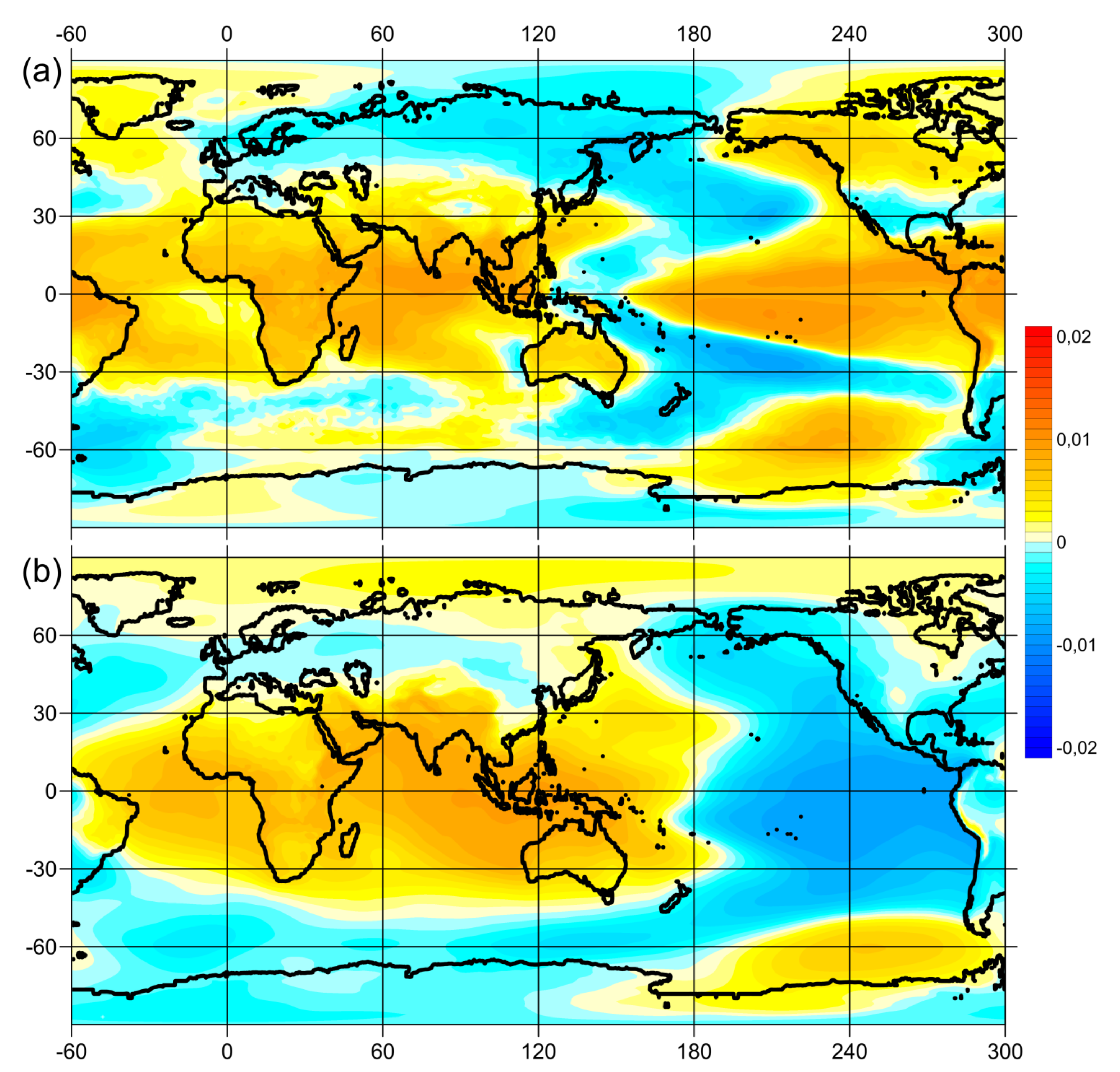
Methods to identify the modes of climatic variability have been studied by different authors; for example, principal component analysis (PCA) with various modifications and improvements based on nonlinearity and the theory of dynamical systems was applied in [64]. We applied PCA, also called empirical orthogonal function (EOF) analysis, to find the EOF1 of the variability of TAS and SLP anomalies at interannual periods inherent in the GAO and ENSO (Figure 1). For this purpose, preliminary band-pass filtering was performed with a Butterworth filter for 2–7 years of the series of TAS and SLP anomalies at each node of the 20CRv3 grid. In addition, to suppress the strong variability of the TAS and SLP anomalies at high latitudes compared to the tropics, the time series at each grid point were normalized to their standard deviations. After that, PCA was applied to the obtained filtered and normalized fields.
The Global Atmospheric Oscillation (GAO) can be characterized by the GAO index (GAO1), which is calculated as the sum of the normalized values of SLP anomalies in 10 geographic regions that coincide with extremes (maxima and minima) in the global EOF1 field of SLP anomaly variability at interannual periods (Figure 1b). The GAO index is calculated using the following formula: GAO1 = P(5° S–5° N, 145°–155° E) + P(5° S–5° N, 55°–65° E) + P(5° S–5° N, 35°–25° W) + P(55°–65° N, 95°–85° W) + P(65°–55°S, 95°–85° W) − P(5° S–5° N, 95°–85° W) − P(45°–55° N, 175°–165° W) − P(45°–55° N, 15°–5° W) − P(55°–45° S, 15°–5° W) − P(55°–45° S, 175°–165° W), where P is the average of SPL anomalies in regions with the given coordinates [54]. When calculating GAO1, the normalized values of SLP anomalies in each region are used to equalize their contributions to the final index. Since the GAO1 values are dimensionless, for the convenience of working with this index, it is normalized to its standard deviation.
Since the SPL anomalies in the equatorial regions of the Pacific Ocean (5° S–5° N, 145°–155° E) and (5° S–5° N, 95°–85° W) are used to calculate the equatorial Southern Oscillation index, in order to separate the GAO from the SO, these regions can be excluded from GAO1. Thus, the GAO index without SO is calculated from the SLP anomalies in eight regions using the following formula: GAO2 = P(5° S–5° N, 55°–65° E) + P(5° S–5° N, 35°–25° W) + P(55°–65° N, 95°–85° W) + P(65°–55° S, 95°–85° W) − P(45°–55° N, 175°–165° W) − P(45°–55° N, 15°–5° W) − P(55°–45° S, 15°–5° W) − P(55°–45° S, 175°–165° W), where P is the average of SPL anomalies in the regions with the given coordinates [54]. Thus, the GAO2 index includes the series of SLP anomalies in eight regions normalized to their standard deviations; that is, SLP anomalies in all eight participating regions make comparable contributions to the GAO2 index. This GAO index without SO (GAO2) is normalized to its standard deviation and is used as the GAO index in this work.
The average oscillation amplitudes of the anomalies of the studied hydrometeorological characteristics between the opposite phases of the GAO were calculated as follows. If the GAO2 values were greater (less) or equal to +0.5 (−0.5) for 5 months or more, then this period of time was attributed to the positive (negative) phase of the GAO. Thus, for the studied period (1900–2015), 30 positive and 25 negative phases of the GAO were identified. The average values of the anomalies of the studied characteristics were calculated for each time interval selected in this way. The mean values and variances were calculated for the obtained two sets of mean values of the anomalies of the studied characteristics at positive and negative phases of the GAO. They were used to calculate the oscillation amplitudes of the anomalies of the studied characteristics between the average positive and average negative phases of the GAO, and using Student’s t-test, their statistical significance was assessed.
Wavelet analysis is useful for analyzing nonstationary signals. A cross-wavelet analysis of the calculated indices GAO2 and EONI was performed using the Morlet wavelet function [65]. Therefore, the complex form of the continuous wavelet transform C(a,b) is C(a,b) = C(a,b)Re + C(a,b)Im at scales a and positions b. To estimate the cross-correlations of the two time series x and y based on the calendar time and time scales of oscillations, the products of their real wavelet components were calculated as follows: Cxy(a,b) = Cx(a,b)Re × Cy(a,b)Re [55,66,67].
Additionally, the magnitude-squared wavelet coherence, which is a measure of the correlation between signals x and y in the time–frequency plane, was calculated [68]. The wavelet coherence of two time series x and y is: |S(C*x(a,b)Cy(a,b))|2/S(|Cx(a,b)|2)·S(|Cy(a,b)|2), where Cx(a,b) and Cy(a,b) denote the continuous wavelet transforms of x and y at scales a and positions b. The superscript * is the complex conjugate, and S is a smoothing operator in time and scale. For real-valued time series, the wavelet coherence is complex-valued if a complex-valued analytic Morlet wavelet is used.
For the wavelet coherence calculation, the “wcoherence” function of MATLAB ver. R2017b was used (https://www.mathworks.com/help/wavelet/ref/wcoherence.html (accessed on 20 October 2021)). All other data mining was performed by using programs written by the authors of the manuscript. The wavelet coherence is computed using the analytic Morlet wavelet. Due to the inverse relationship between frequency and period, a plot that uses the sampling interval is the inverse of a plot that uses the sampling frequency. For areas where the coherence exceeds 0.5, plots that use the sampling frequency display arrows to show the phase lag of y with respect to x. The arrows are spaced in time and scale. The direction of an arrow corresponds to the phase lag on the unit circle. For example, a vertical arrow indicates a π/2 or quarter-cycle phase lag. The corresponding lag in time depends on the duration of the cycle.
3. Results and Discussion
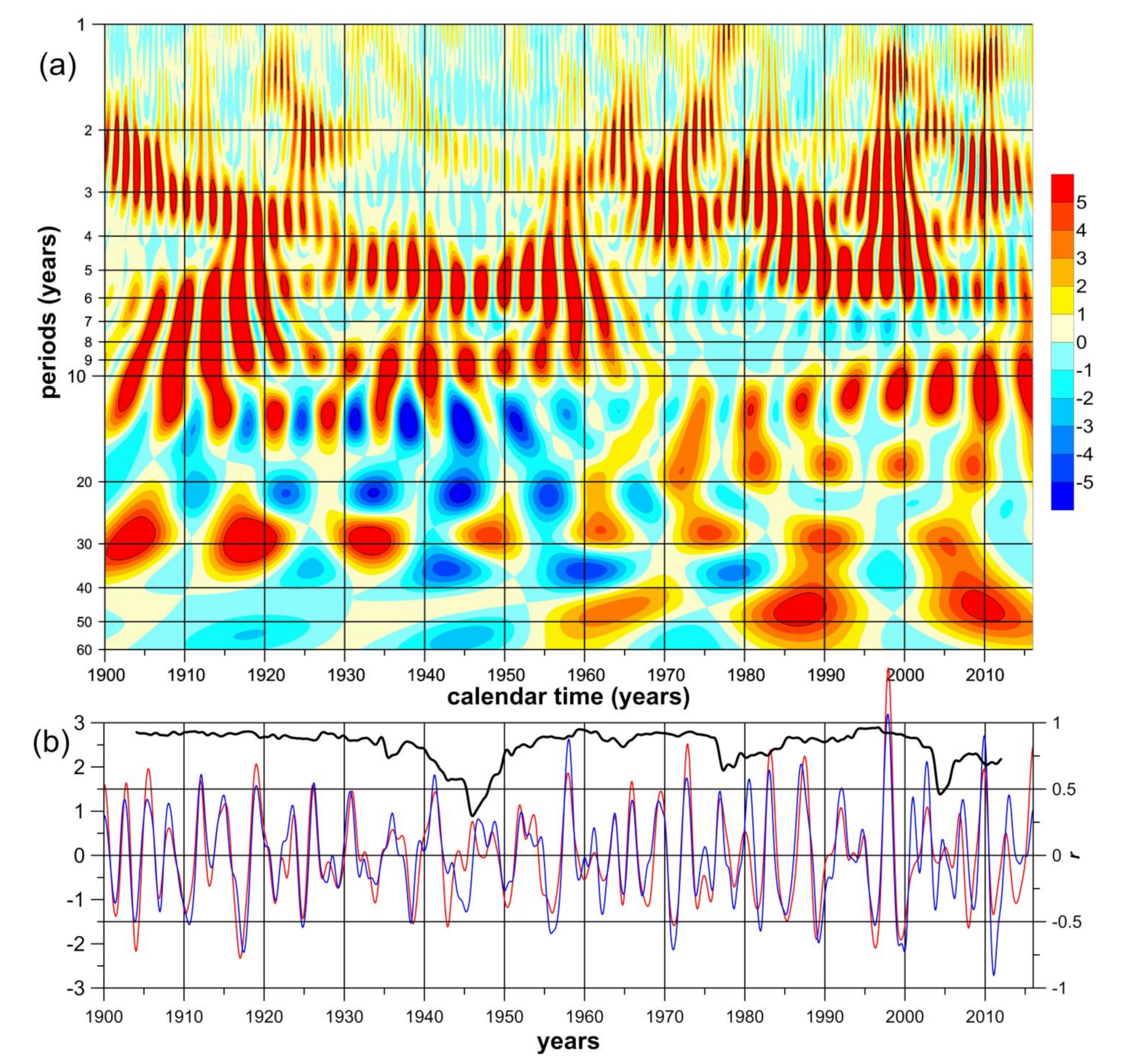
To assess the links between the GAO and ENSO, a cross-wavelet analysis of the calculated indices GAO2 and EONI was performed (Figure 2a). The cross-wavelet diagram of GAO2 and EONI (Figure 2a) allows the identification of temporal variations that determine their large cross-correlations. The red regions in this wavelet diagram indicate an almost complete coincidence between the phases of the GAO2 and EONI variations. The areas marked in blue correspond to the out-of-phase behavior of these indices. As can be seen, the red areas cover a significant part of the GAO2 and EONI cross-wavelet diagram on time scales from 2 to 7 years. However, there are calendar intervals in which the links between GAO2 and EONI are weakened in some periods of fluctuations and strengthened in other periods. The wavelet coherence of GAO2 and EONI (Supplementary Materials Figure S1) shows similar results to the cross-wavelet diagram (Figure 2a).
The time series of GAO2 and EONI with Butterworth band-pass filtering from 2 to 7 years and sliding cross-correlations between them with a window of 8 years (Figure 2b) demonstrate strong links between the GAO and ENSO on interannual time scales. The observed weakening of these links in the 1940s can be attributed to the paucity of observational data during World War II. When calculating cross-correlations with a window of 8 years, the length of the series involved in obtaining individual correlation values was 96 values (8 times 12 months). However, after applying band-pass filtering, these 96 values can no longer be considered independent, and therefore, the given values of the correlations are purely illustrative and not evaluative. Since even white noise can become cyclical after applying band-pass filtering, the results presented in Figure 2b should be considered an addition to the cross-wavelet diagram, which is shown in Figure 2a, and were not subjected to band filtering of the rows after the data were obtained.
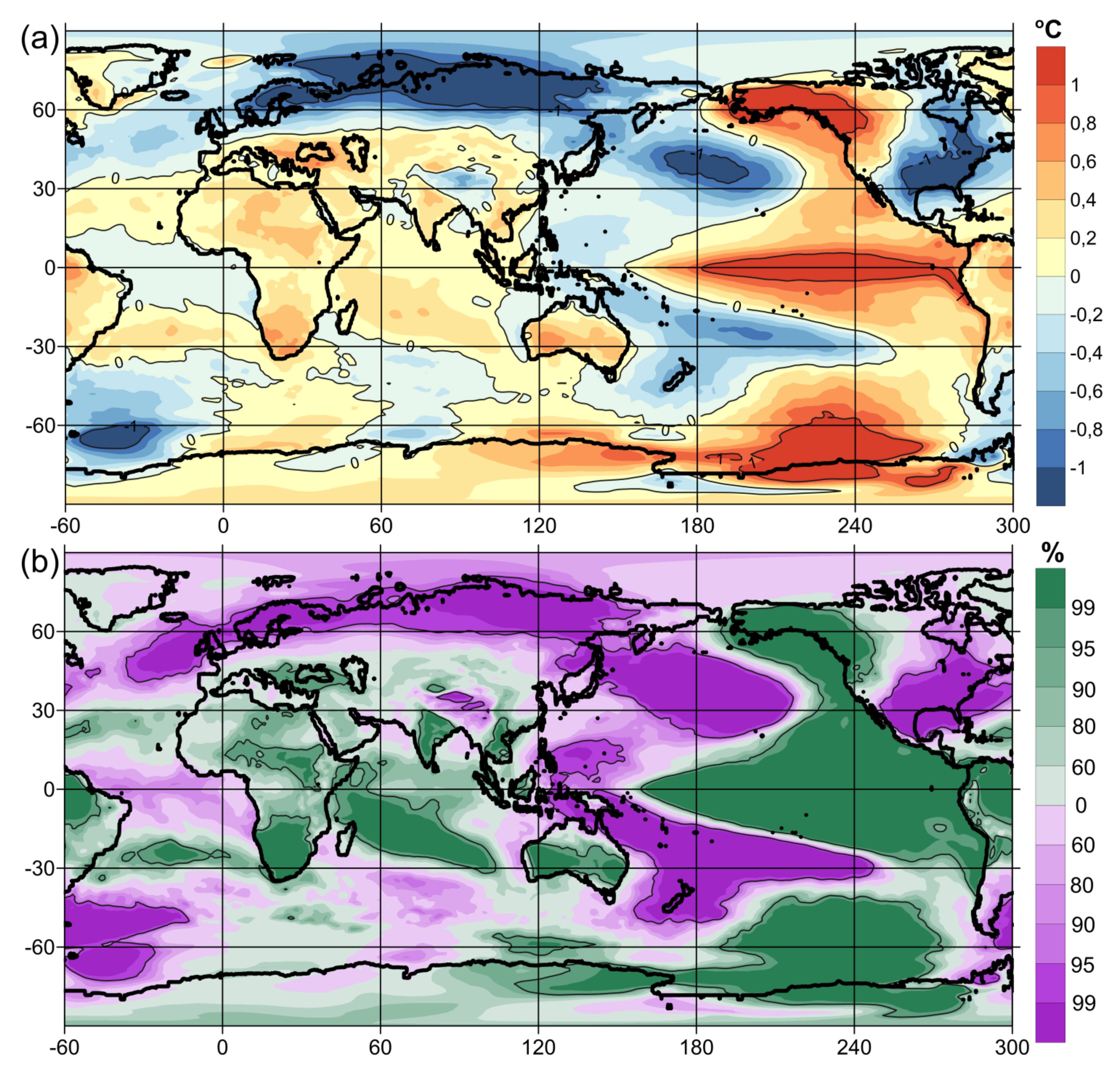
Figure 3 maps the oscillation amplitudes of the mean air temperature anomalies at the surface (TAS) between the opposite phases of the GAO and Student’s t-criterion. TAS anomalies form a global structure that is symmetrical about the equator, taking into account the location of the continents. Along the equator of the central and eastern parts of the Pacific Ocean, positive TAS anomalies are observed, which are typical for El Niño. Weaker values of above-zero anomalies extend from the equator to the north and south along the coasts of the Americas. Reaching high latitudes, they intensify and form two regions of positive TAS anomalies located symmetrically relative to the equator over Alaska and the Amundsen Sea. The wavelet coherence between GAO2 and TAS anomalies in the Amundsen Sea region (55°–70° S, 150°–100° W) (Supplementary Materials Figure S2) is higher than that between GAO2 and TAS anomalies in the Alaska region (55°–70° N, 170°–120° W) (Supplementary Materials Figure S3), which may be the result of the ocean–atmosphere interaction in the Amundsen Sea region.
Negative TAS anomalies are located in the western part of the Pacific Ocean with two centers in the middle latitudes of its northern and southern parts. The wavelet coherence between GAO2 and TAS anomalies in northern (30°–45° N, 160° E–160° W) (Supplementary Materials Figure S4) and southern (20°–35° S, 160° E–150° W) (Supplementary Materials Figure S5) regions of the western Pacific Ocean middle latitudes is high at periods of 2–7 years throughout the 1900–2015 time interval. However, this is not surprising, since these regions are close to the tropics of the Pacific Ocean, where ENSO events are observed.
TAS anomalies in the Indian Ocean region—Hindustan Peninsula, Southeast Asia, the west of the Indonesian archipelago, Australia, Africa and the Arabian Peninsula—are mostly positive, with the exception of the south and southeast of the Indian Ocean off the coast of Australia, as well as the Tibetan Plateau region, where negative TAS anomalies are observed. The wavelet coherence between GAO2 and TAS anomalies in the Indian Ocean region (0°–20° S, 50°–90° E) (Supplementary Materials Figure S6) has a gap in its high values in the 1940s, which may be the result of the lack of observations in this region during World War II. In addition, the wavelet coherence between GAO2 and TAS anomalies in the Indian Ocean region is higher at periods of about 2–4 years than at 5–7 years. The wavelet coherence between GAO2 and TAS anomalies in the Hindustan Peninsula region (10°–30° N, 75°–85° E) (Supplementary Materials Figure S7) has higher values than that between GAO2 and TAS anomalies in Australia (20°–35° S, 120°–150° E) (Supplementary Materials Figure S8) or Southern Africa (15°–30° S, 20°–30° E) (Supplementary Materials Figure S9) regions.
In the tropical region of the Atlantic Ocean, negative TAS anomalies are observed, which transform into positive anomalies in the northern and southern subtropics and then revert to negative anomalies in middle and high latitudes. However, the wavelet coherence between GAO2 and TAS anomalies in high latitudes of the Southern Atlantic region (70°–60° S, 60°–30° W) (Supplementary Materials Figure S10) has a lot of gaps at 2–7-year periods over the 1900–2015 calendar interval. The above-mentioned positive TAS anomalies are located in the northwestern part of North America. At the same time, negative TAS anomalies are observed in the southern and eastern parts of North America. The South American continent is predominantly occupied by positive TAS anomalies, with the exception of its southern part. The wavelet coherence between GAO2 and TAS anomalies in the South American continent region (15° S–5° N, 70°–50° W) (Supplementary Materials Figure S11) is higher than that between GAO2 and TAS anomalies in the southern and eastern parts of the North American region (25°–45° N, 105°–70° W) (Supplementary Materials Figure S12).
In the northern part of Eurasia and the Arctic, negative TAS anomalies are observed. In the southern part of Eurasia, including the Mediterranean, Black and Caspian Seas, positive TAS anomalies are observed, with the exception of the previously mentioned region of the Tibetan Plateau. However, the wavelet coherence between GAO2 and TAS anomalies in the northern part of Eurasia and the Arctic (60°–80° N, 10°–150° E) (Supplementary Materials Figure S13) and the Black and Caspian Sea regions (35°–45° N, 25°–50° E) (Supplementary Materials Figure S14) is low at 2–7-year periods and unstable throughout the 1900–2015 calendar interval. TAS anomalies in Antarctica are predominantly positive, but they are not very reliable due to the extremely small number of observations in this region.
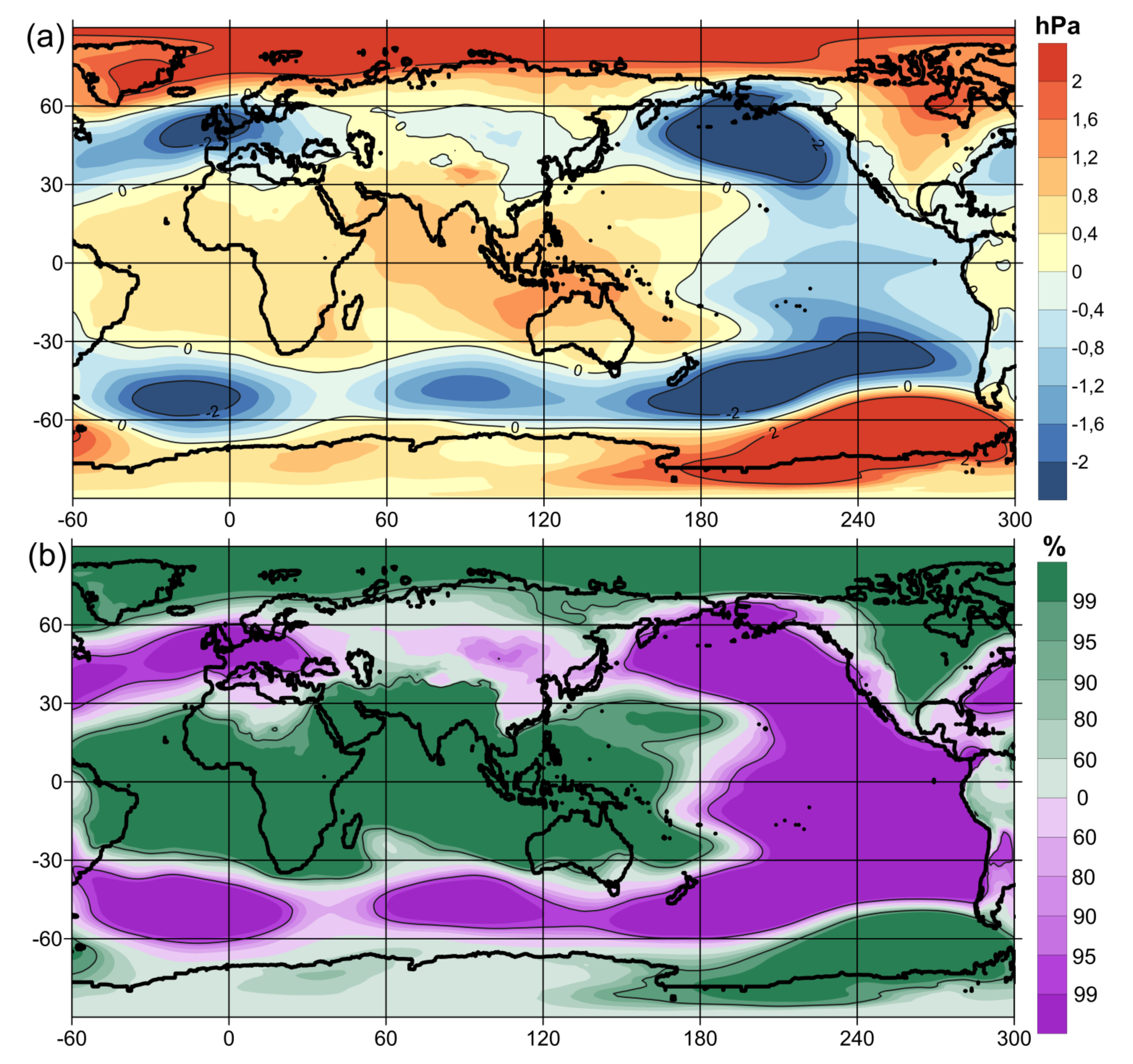
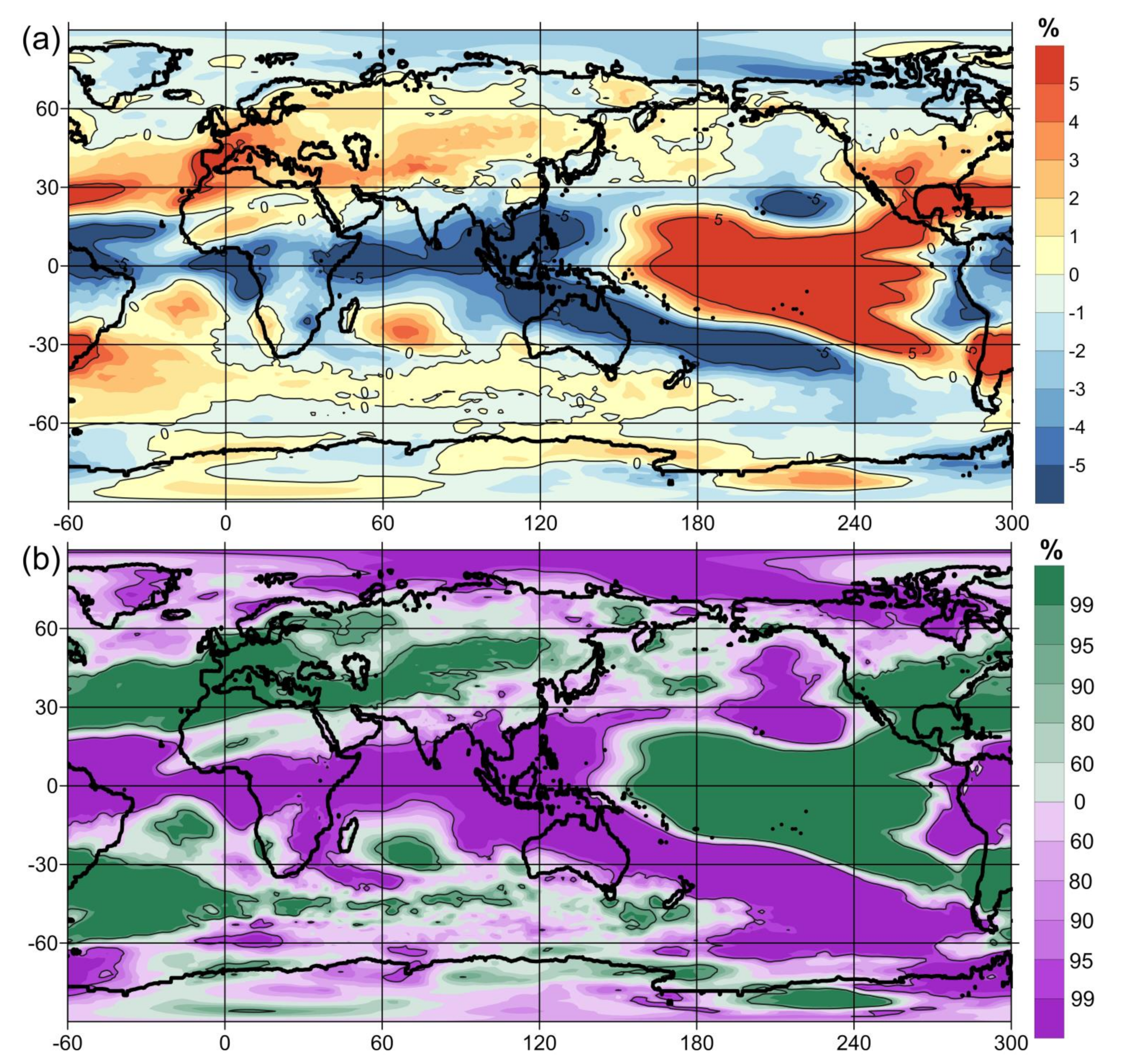
The global spatial structure of the oscillation amplitudes of mean sea level pressure (SLP) anomalies between the opposite phases of the GAO has symmetry, both relative to the equator and relative to the 90° W meridian (Figure 4). A vast area of positive SLP anomalies is observed in the low latitudes of South America, the Atlantic Ocean, Africa, the Indian Ocean region, the Indonesian archipelago, Australia and the western part of the Pacific Ocean. The wavelet coherence between GAO2 and SLP anomalies in this region (30° S–30° N, 50° W–170° E) has high values at interannual periods throughout the 1900–2015 calendar interval (Supplementary Materials Figure S15). This is because the GAO2 index includes SLP anomalies in (5° S–5° N, 55°–65° E) and (5° S–5° N, 35°–25° W) regions.
In the middle latitudes, this large region of positive SLP anomalies is bordered by regions of negative SLP anomalies, which form an X-shaped structure with the center of intersection at the equator of the central-eastern part of the Pacific Ocean. The main centers of negative SLP anomalies are located in the middle latitudes of the Pacific, Atlantic and Indian Oceans. The wavelet coherence between GAO2 and SLP anomalies in middle latitudes of the northern (45°–55° N, 175°–165° W) (Supplementary Materials Figure S16) and southern (55°–45° S, 175°–165° W) (Supplementary Materials Figure S17) regions of the Pacific Ocean and in middle latitudes of the northern (45°–55° N, 15°–5° W) (Supplementary Materials Figure S18) and southern (55°–45° S, 15°–5° W) (Supplementary Materials Figure S19) regions of the Atlantic Ocean has high values at interannual periods, but a lot of gaps are evident during the 1900–2015 calendar interval. In the center and east of Asia, negative SLP anomalies are also observed, but they are much weaker than the centers of negative SLP anomalies over the oceans, which may serve as evidence of the leading role of the ocean–atmosphere interaction in the physical mechanism of the GAO.
At high latitudes to the north and south of the center of the intersection between the branches of the X-shaped structure of negative SLP anomalies, there are two regions of positive SLP anomalies. The first region covers most of North America and the entire Arctic, and the second one—the region of the Amundsen, Bellingshausen and Weddell Seas—covers all of Antarctica. The wavelet coherence between GAO2 and SLP anomalies in the Amundsen, Bellingshausen and Weddell Sea region (70°–55° S, 130°–70° W) (Supplementary Materials Figure S20) is higher than in the North American region (40°–70° N, 110°–80° W) (Supplementary Materials Figure S21), which may be the result of the ocean–atmosphere interaction.
In many respects, the fields of the oscillation amplitudes of the mean TAS (Figure 3) and SLP (Figure 4) anomalies between opposite GAO phases turned out to be similar to those of the EOF1 of the interannual variability of TAS and SLP anomalies (Figure 1). However, the application of the principal component method (Figure 1) implies that the analysis includes all data of the TAS and SLP anomalies, including those corresponding to the neutral states of the GAO and ENSO. The spatial structures of the TAS and SLP anomalies inherent in the neutral states of the GAO and ENSO are inhomogeneous. Therefore, when used in the analysis, they reduce the calculated values of cross-correlations, for example, in [43]. On the contrary, the composite analysis used to obtain the fields of the oscillation amplitudes of the mean TAS (Figure 3) and SLP (Figure 4) anomalies between the opposite GAO phases does not include neutral states of the GAO and ENSO and thus only accounts for differences between more homogeneous TAS and SLP anomalies associated with opposite phases of the GAO (El Niño and La Niña). Therefore, in order to suppress the inhomogeneity of the neutral states of the GAO, when constructing the fields of principal components (Figure 1), band-pass filtering from 2 to 7 years was applied, which contributes to the isolation of the GAO variability.
The main differences between the EOF1-field of the interannual variability of the TAS anomalies presented in Figure 1a and the field of oscillation amplitudes of mean TAS anomalies between opposite phases of the GAO (Figure 3) are observed in the tropics of the Atlantic Ocean. Perhaps this is because the wave property of the GAO propagates from west to east [44,45,46,47,54], which is also shown below. The PCA method displays the later phase of the GAO, when the TAS anomalies in the tropics of the Pacific Ocean have already influenced the tropics of the Atlantic Ocean, causing the TAS anomalies of the regions to adopt the same sign. There are no such significant differences in the fields of the SPL anomalies (Figure 1b and Figure 4), with the exception of the regions of North America and Eurasia. However, over the continents, GAO anomalies are much less pronounced and more unstable than over the oceans because the GAO is a process of interaction between the ocean and the atmosphere. Without the inertia (memory) of the ocean, high-frequency atmospheric disturbances rapidly destroy the spatial structure of the GAO.
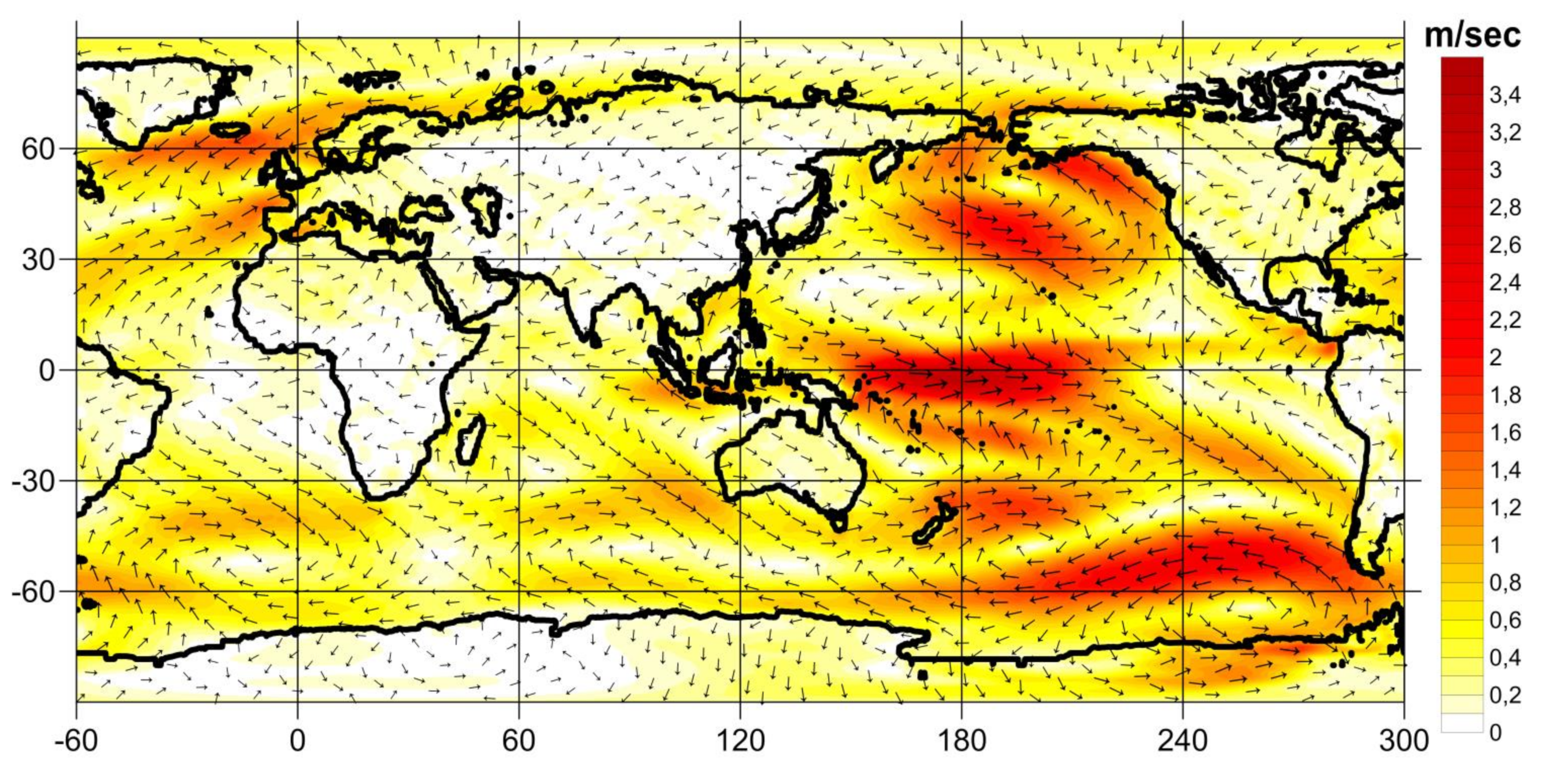
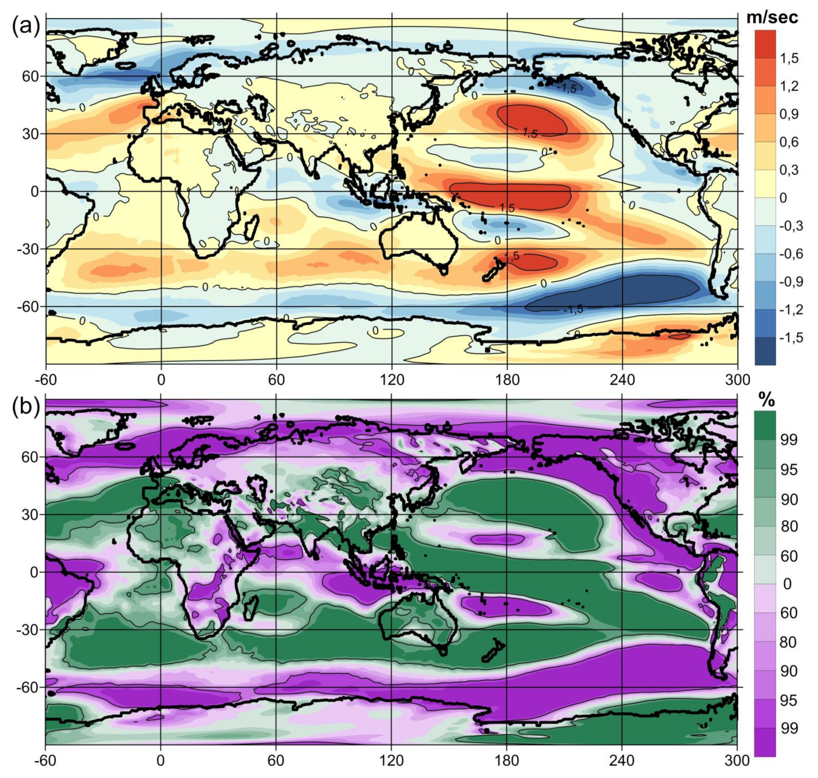
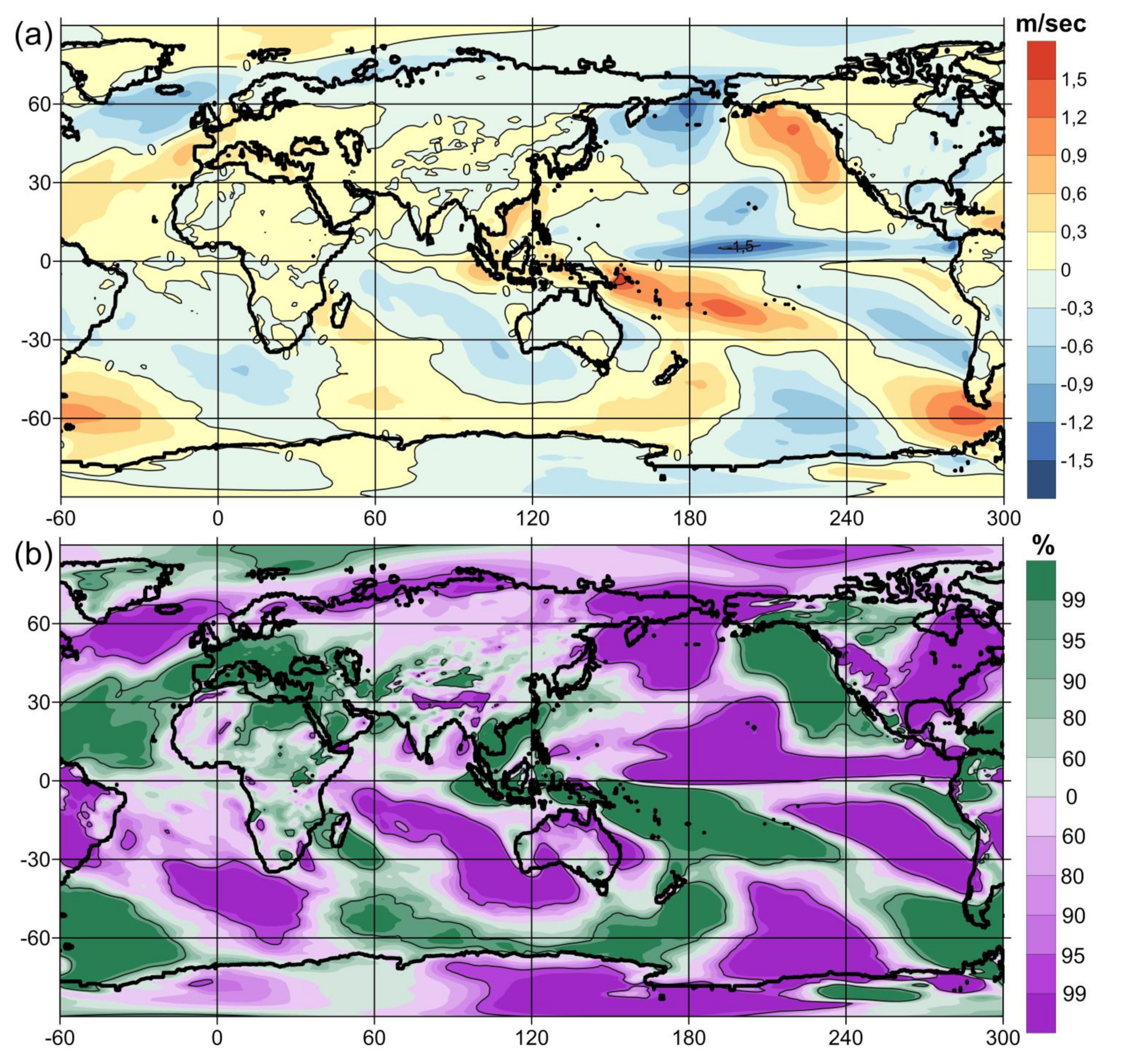
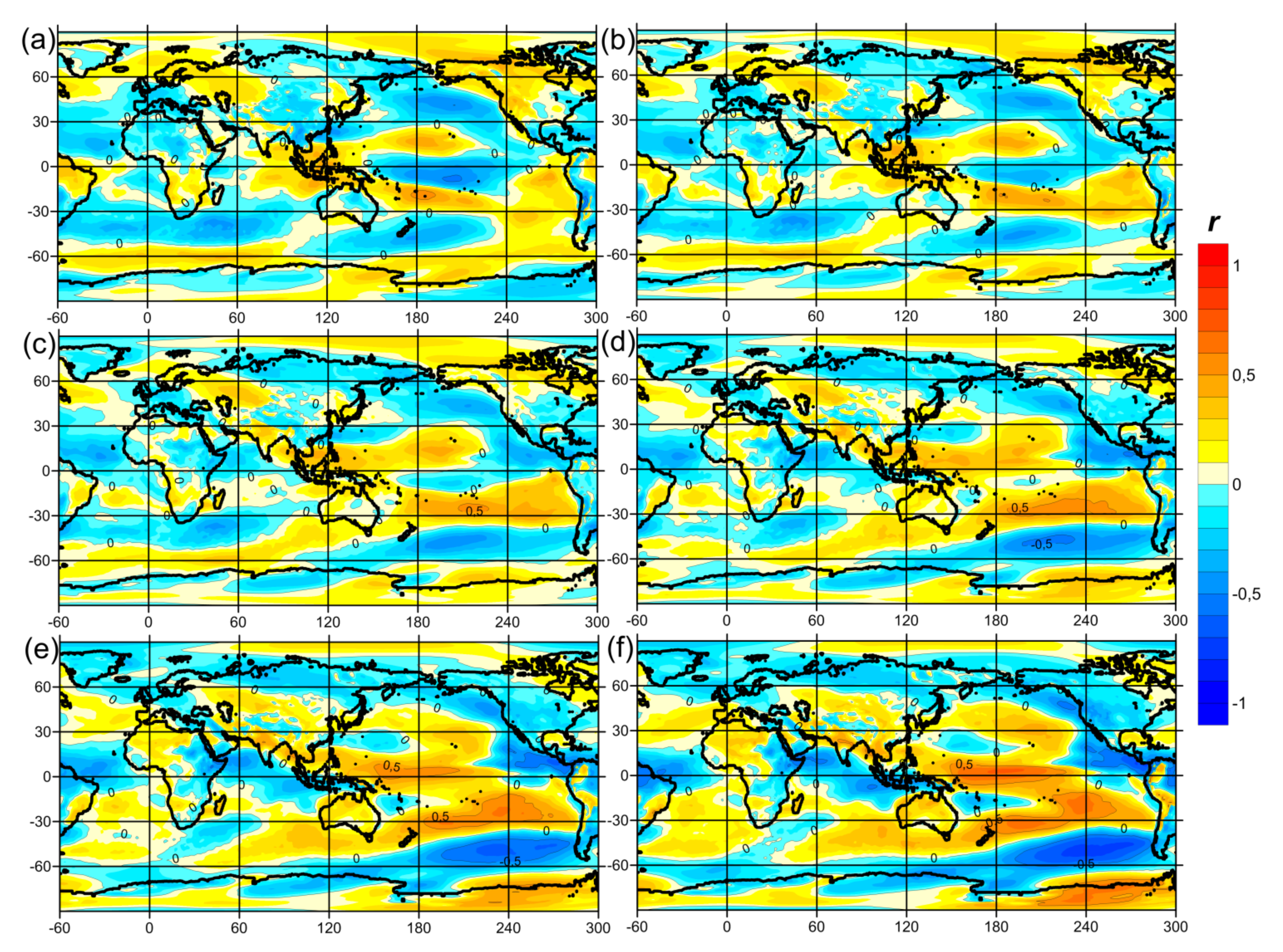
Figure 5 shows the field of oscillation amplitudes of the mean wind speed anomalies near the surface (SWS) between the opposite phases of the GAO, and Figure 6 and Figure 7 show the fields of its zonal and meridional components. In the western and central parts of the near-equatorial region of the Pacific Ocean, anomalies of the westerly wind are observed, characteristic of weakened Pacific trade winds. Figure 4 shows negative anomalies of the SPL in the Aleutian minimum region. The SWS anomalies correspond to these negative SLP anomalies and form the cyclonic SWS anomaly in the North Pacific Ocean. In the region of the South Pacific that is symmetrically located relative to the equator, a cyclonic anomaly of the SWS is also observed but is slightly smaller in size. It is possible that its smaller spatial scales are associated with the adjacent positive SLP anomalies and the anticyclonic SWS anomaly in the region of the Amundsen, Bellingshausen and Weddell Seas. In the North American region, however, such large-scale anomalies of the SLP and SWS are not observed, which confirms the decisive role of the interaction between the ocean and the atmosphere in the formation of the GAO.
In the tropics of the Indian Ocean, SWS anomalies are observed, characteristic of the reverse of the Walker circulation cell in this region, with the largest east wind anomalies off the coast of Sumatra. However, these easterly wind anomalies do not cause the SAT anomalies characteristic of the Indian Ocean Dipole (IOD) (Figure 3). As shown in [55], the largest temperature anomalies characteristic of IOD occur during the positive phase of the GAO at depths of 50–100 m due to a rise in the thermocline off the coast of Sumatra. In the middle latitudes of the southern part of the Indian Ocean, cyclonic anomalies of SWS are observed, corresponding to negative anomalies of SPL in this region.
In the middle and high latitudes of the North Atlantic, there is a cyclonic SWS anomaly centered over the British Isles (Figure 5). It corresponds to the NAO-like structure of the SPL anomalies (Figure 4); however, it shifts somewhat to the southwest in comparison with the spatial structure of the NAO, with the center of negative SLP anomalies in the Icelandic minimum region with a positive NAO phase. Thus, the northeastern wind anomalies arising during the positive phase of the GAO impede the transfer of heat and moisture from the North Atlantic to the northern part of Eurasia and the Arctic and cause negative SAT anomalies in this vast region (Figure 3). Cyclonic SWS anomalies in the Aleutian Minimum region with northerly wind anomalies in its western part, covering the region of northeast Asia, also contribute to negative SAT anomalies in northeast Asia. The northeastern wind anomalies and negative SAT anomalies observed in the Greenland Sea and Labrador Sea during the positive phase of the GAO may cause an intensification of deep convection in this region.
While the northern part of the cyclonic SWS anomaly centered over the British Isles causes negative TAS anomalies in northern Eurasia during periods of positive GAO phases, the southern part of this cyclonic anomaly, due to southwestern wind anomalies, contributes to positive TAS anomalies in southern Europe; Mediterranean, Black and Caspian Seas; and Central Asia region. The region of cyclonic anomalies of the SWS is also located almost symmetrically relative to the equator in the high and middle latitudes of the southern part of the Atlantic Ocean. In its western part, southerly wind anomalies cause negative TAS anomalies in the Weddell Sea region, thereby contributing to the occurrence of deep convection in its ice-free part.
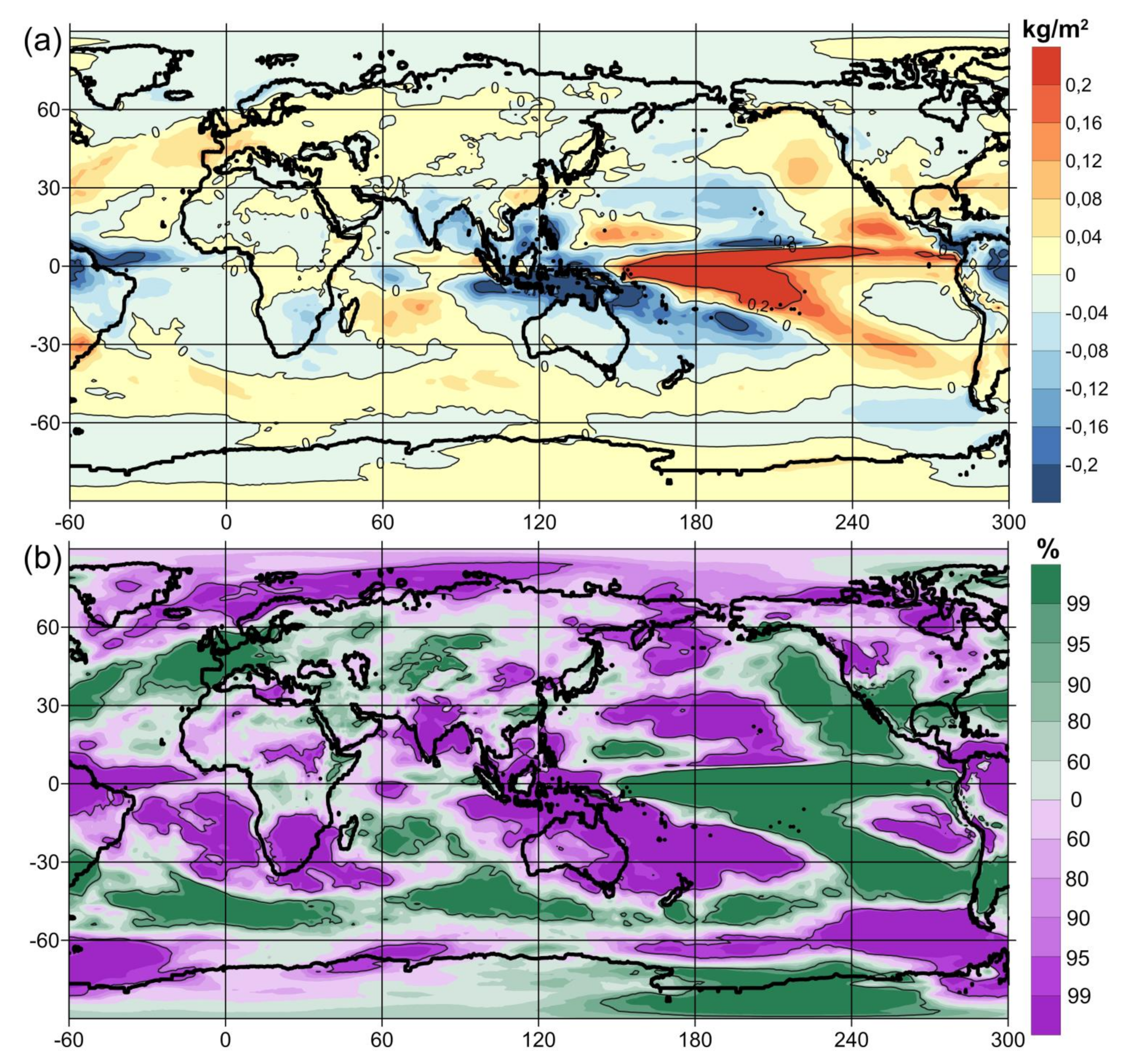
The largest amplitudes of fluctuations in the total amount of precipitation (TAP) between the positive and negative GAO phases are observed in the tropical belt of the Earth (Figure 8). During the positive phase of the GAO in the tropics of the Atlantic Ocean, the regions of the Indian subcontinent, South Africa, the Indonesian archipelago, Australia and the tropics of South and Central America, less precipitation falls than during the periods of the negative GAO. In [69], using a climate model of intermediate complexity, a physical mechanism was identified, which, according to the authors, is the reason for the regional decrease in precipitation at the edges of convective zones during El Niño (positive phase of GAO). According to this mechanism, a warm troposphere increases the moisture content of the surface boundary layer, which is necessary for convection to occur. In regions where moisture is abundant, warm and humid air rises to support rainfall, but this increases the moisture gradient relative to neighboring areas. Thus, a decrease in the amount of precipitation occurs at the edges of the convective zones. This mechanism is the main cause of drought in some tropical regions during El Niño. Positive TAP anomalies during the positive GAO phase are observed in the near-equatorial zone of the Pacific Ocean, and in some regions, negative TAP anomalies are observed at the edges of this zone (Figure 8). Positive TAP anomalies are observed in the middle latitudes of the Atlantic, Indian and Pacific Oceans, with the exception of the western part of the Pacific Ocean. During the positive GAO phase, positive TAP anomalies are also observed in Europe and Central Asia.
TAP anomalies correlate well with total cloud cover (TCC) anomalies (Figure 9). Positive TCC anomalies are located in the tropics of the central part of the Pacific Ocean, in the region where the planetary convection region shifts during El Niño. Negative TCC anomalies are located in the tropical regions of Indonesia, Australia, the Indian Ocean, the Indian subcontinent, Africa, the Atlantic and South America. Positive TCC anomalies during the positive phase of the GAO are observed in the middle latitudes of the Atlantic Ocean, North and South America, and Eurasia, where positive TAP anomalies are also located.
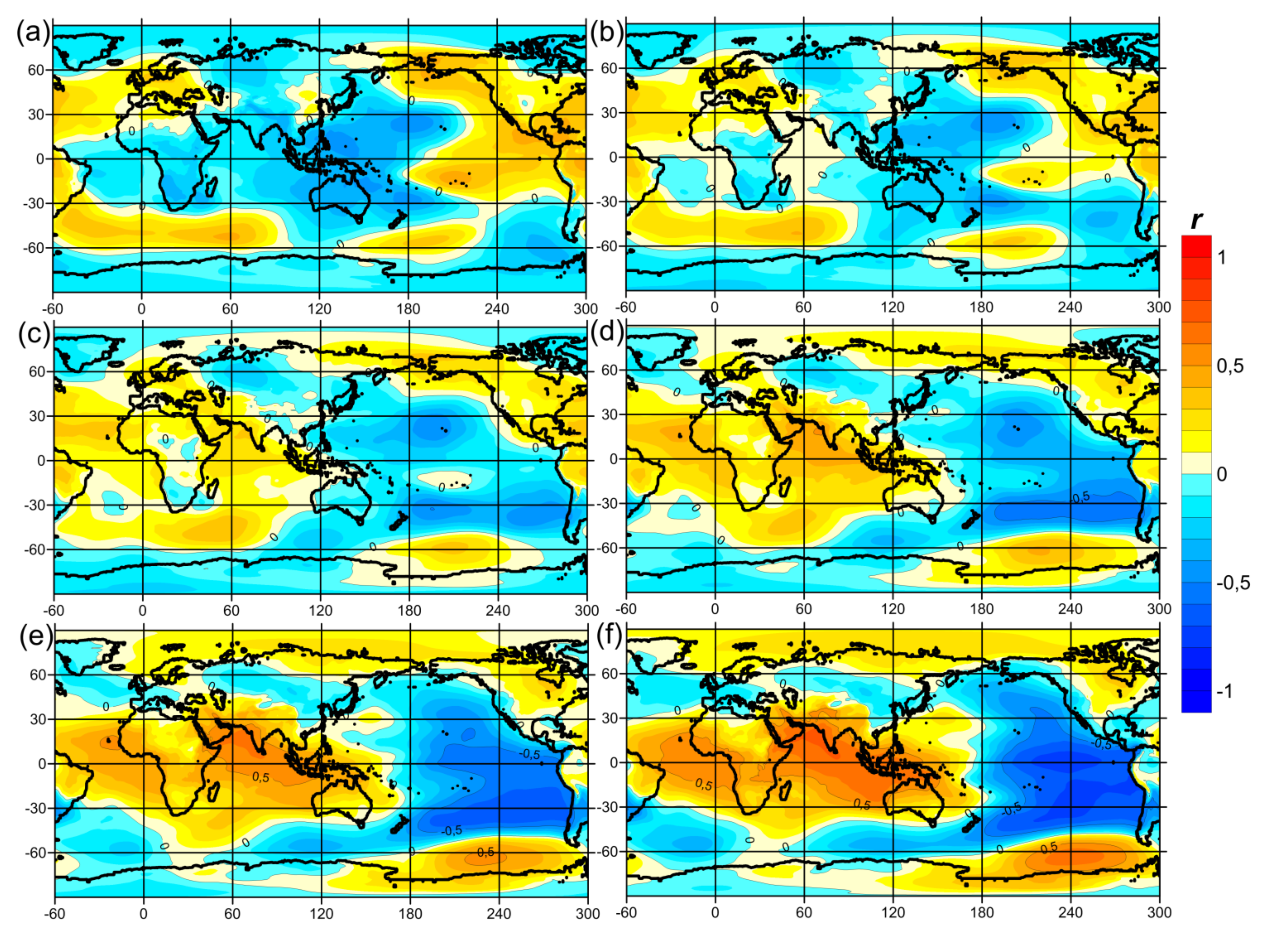
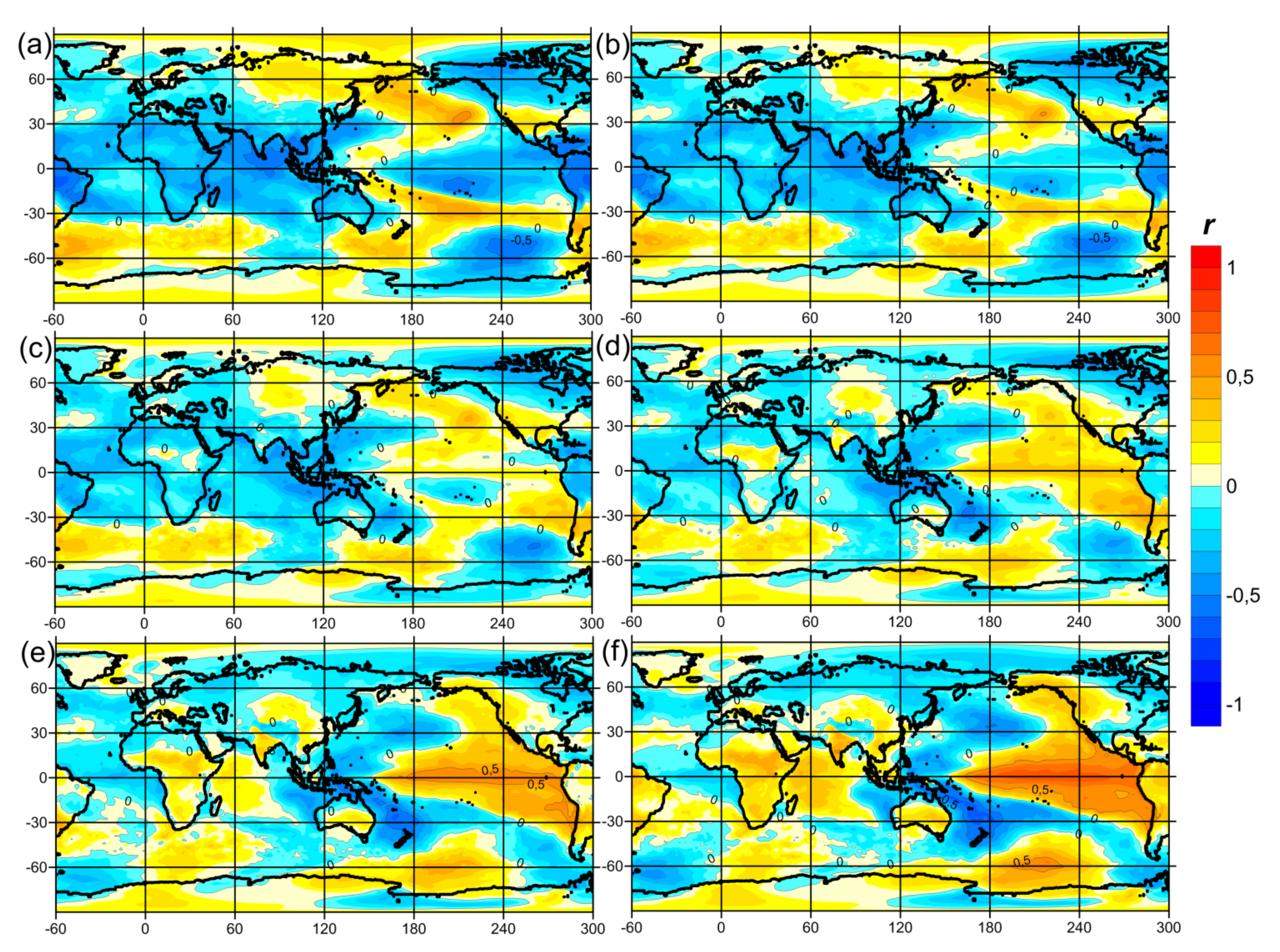
The physical mechanism of the GAO can be briefly formulated as follows: during the negative phase of the GAO (Figure 10a and Figure 11a), negative SAT anomalies are observed in the tropics of the Indian and Atlantic Oceans, the African continent and the Indonesian archipelago (Figure 11a–c). In this vast region of negative TAS anomalies, the SPL begins to increase, and in the surrounding middle latitudes, negative SPL anomalies appear—the transition of the GAO to its positive phase (Figure 10b–f). The positive SPL anomalies arising in the region of the Indonesian archipelago (Figure 10c–e) cause the displacement of the western SWS anomalies, shifting from this region to the east to the central part of the equatorial region of the Pacific Ocean (Figure 12c–e), thereby causing a weakening of the Pacific trade winds and triggering the process of El Niño initiation, which further develops due to the Bjerknes feedback and the interaction of Kelvin and Rossby waves. The teleconnections of the strengthened El Niño due to changes in the Walker circulation in turn cause an increase in TAS in the tropics of the Indian Ocean and the African continent (Figure 11e,f), which leads to negative SPL anomalies in these regions and the transition of the GAO back to its negative phase.
As a hypothesis, the eastward propagation of GAO SLP and TAS anomalies (Figure 10 and Figure 11) can be explained by the influence of the Chandler wobble on the movement of the poles of the Earth. The Chandler wobble excites tidal waves (pole tides) in the atmosphere and oceans, propagating from west to east in middle latitudes in antiphase in both hemispheres [70,71]. The analyses of satellite data on the sea surface temperature (SST) and sea surface height (SSH) anomalies of the Pacific Ocean carried out in [63,72] showed that the North Pacific pole tide, after its reflection from the west coast of Central America, causes positive SST and SSH anomalies in the equatorial region of the Pacific Ocean. Thus, this pole tide can be considered an El Niño trigger [72,73]. The continents are not an insurmountable obstacle to the propagation of atmospheric pole tides from west to east. Consequently, since the GAO is affected by the Chandler wobble, it can be expected that the spatial features in the extratropical components of the GAO should also propagate from west to east. Based on this west-to-east spread of the GAO, a predictor index was proposed in [54,66,67] to predict El Niño and La Niña events with a lead time of about one year. Nevertheless, it should be noted that further studies are required to verify the statement that the eastward propagation of anomalies connected with the GAO is induced by the pole tides.
Seasonality plays an important role in GAO correlations and remote responses to ENSO. Strong correlations were found at the 1.5-year period between variations in the Indian Ocean Dipole (IOD) and ENSO [55], which is the result of the seasonality of these phenomena. In [67], it was shown that predicting ENSO based on the eastward propagation of the GAO could help to overcome the well-known spring predictability barrier (SPB) of ENSO forecasting. Additionally, based on various data, in [63,74], the power spectra of GAO and ENSO indices revealed numerous peaks not only at periods caused by the seasonality but also at the sub-harmonics of the 14-month Chandler wobble in the movement of the Earth’s poles and the super-harmonics of the 18.6-year lunisolar nutation of the Earth’s rotation axis and 11-year sunspot activity. Due to the incommensurability of their periods, all of these external forces act on the climate system at different points in time. As a result, the shape of the power spectra of GAO and ENSO indices looks very complex. It reveals numerous peaks located at multiples of the above periodicities, as well as their sub- and super-harmonics. However, the detected peaks may be random due to the short time series of available observations and may disappear in the future.
The interaction of oceanic baroclinic waves (equatorial Kelvin and Rossby waves and off-equatorial Rossby waves), described by the theory of a “delayed oscillator” [75], plays an important role in the physical mechanism of ENSO. The movement of oceanic Kelvin and Rossby waves with a deep or elevated thermocline and their reflection from the boundaries in the west and east of the Pacific Ocean forms a cycle of oscillations, which is expressed in the change in the surface temperature of the equatorial part of the Pacific Ocean. In [76], it was shown that these oceanic baroclinic waves form a single dynamical system whose average period is 4 years (the effective period varies between 1.5 and 7 years). This quadrennial quasi-stationary wave (QSW) is coupled to an annual QSW formed by a first baroclinic, fourth meridional mode equatorial Rossby wave. The annual QSW is resonantly forced by easterlies, while the quadrennial QSW is partly forced by ENSO, which is a component of the GAO.
ENSO is characterized based on the date that the events are mature. Their time lag, defined relative to the central value of successive intervals of 4 years, e.g., 1996–2000, affects their evolution and, for a given amplitude, their variability. It determines the dynamics of the quadrennial QSW in the tropical Pacific since ENSO always occurs at the end of the eastward phase propagation of that QSW [77]. This new approach allows specifying the modes of interaction between the atmosphere and the oceanic baroclinic waves of the tropical Pacific Ocean. The Kelvin wave transfers the warm waters of the western tropical Pacific to the east. The stimulation of evaporative processes in the eastern Pacific favors a rise in the thermocline and, consequently, the westward recession of the quadrennial QSW.
4. Conclusions
Modern studies of El Niño–Southern Oscillation (ENSO) teleconnections show an apparent impact of ENSO on various climatic processes occurring in various parts of the Earth, that is, the global influence exerted by ENSO. However, they also show that some climatic processes occurring in various regions of the Earth, which are sometimes quite remote from the tropics of the Pacific Ocean, lead to the onset of El Niño or La Niña events and, as data suggest, may have an impact on ENSO.
The recently discovered Global Atmospheric Oscillation (GAO) includes the ENSO itself, as well as forward and reverse teleconnections between ENSO and anomalies of air temperature at the surface, atmospheric pressure at sea level and wind speed on time scales from 2 to 7 years in different regions of the Earth. The GAO is a planetary mode of interannual climatic variability. The spatial structure of GAO anomalies spreads from west to east, both in the tropical belt of the Earth and in middle and high latitudes.
In this work, the amplitudes of fluctuations of global anomalies of air temperature at the surface, sea-level pressure, wind speed at the surface, total precipitation and total cloudiness between the opposite phases of the GAO are investigated. The global structures of the fields of oscillation amplitudes of these anomalies and their high interconnection with each other are shown. The influence of the GAO on the anomalies of the studied characteristics in different regions of the Earth is described. Student’s t-test was used to estimate the probability of these anomalies.
The physical mechanism by which the transition from the negative to the positive phase of the GAO affects the onset of El Niño events is described. Moreover, the further development of El Niño and the intensification of its anomalies, in turn, affect the transition from the positive to negative phase of the GAO.
It was found that the GAO causes record temperature anomalies in the Arctic and in the north of Eurasia, which can have a significant impact on permafrost and, as a result, on housing, railways, and automobile and pipeline infrastructure in this region of Russia.
The analysis of the wavelet coherence between the GAO index and surface air temperature and sea-level pressure anomalies in different regions of the Earth show that this coherence is higher over the oceans than over the continents. This may be evidence of the important role of the ocean–atmosphere interaction in the physical mechanism of the GAO.
The results show indications that the positive GAO phase has an enhancing effect on deep convection in the Greenland Sea, the Labrador Sea and the Weddell Sea. However, additional studies are required to confirm the effect of the GAO on deep convection in these regions.
Supplementary Materials
The following are available online at https://0-www-mdpi-com.brum.beds.ac.uk/article/10.3390/atmos12111443/s1. Figure S1: The wavelet coherence and phase between GAO2 and EONI for 1900–2015. Figure S2: The wavelet coherence and phase between GAO2 and TAS anomalies in Amundsen Sea region (55°–70°S, 150°–100°W) for 1900–2015. Figure S3: The wavelet coherence and phase between GAO2 and TAS anomalies in Alaska region (55°–70°N, 170°–120°W) for 1900–2015. Figure S4: The wavelet coherence and phase between GAO2 and TAS anomalies in northern part of the western Pacific Ocean middle latitudes region (30°–45°N, 160°E–160°W) for 1900–2015. Figure S5: The wavelet coherence and phase between GAO2 and TAS anomalies in southern part of the western Pacific Ocean middle latitudes region (20°–35°S, 160°E–150°W) for 1900–2015. Figure S6: The wavelet coherence and phase between GAO2 and TAS anomalies in Indian Ocean region (0°–20°S, 50°–90°E) for 1900–2015. Figure S7: The wavelet coherence and phase between GAO2 and TAS anomalies in Hindustan Peninsula region (10°–30°N, 75°–85°E) for 1900–2015. Figure S8: The wavelet coherence and phase between GAO2 and TAS anomalies in Australia region (20°–35°S, 120°–150°E) for 1900–2015. Figure S9: The wavelet coherence and phase between GAO2 and TAS anomalies in Southern Africa region (15°–30°S, 20°–30°E) for 1900–2015. Figure S10: The wavelet coherence and phase between GAO2 and TAS anomalies in high latitudes of Southern Atlantic region (70°–60°S, 60°–30°W) for 1900-2015. Figure S11: The wavelet coherence and phase between GAO2 and TAS anomalies in South American continent region (15°S–5°N, 70°–50°W) for 1900–2015. Figure S12: The wavelet coherence and phase between GAO2 and TAS anomalies in southern and eastern parts of North America region (25°–45°N, 105°–70°W) for 1900–2015. Figure S13: The wavelet coherence and phase between GAO2 and TAS anomalies in the northern part of Eurasia and the Arctic region (60°–80°N, 10°–150°E) for 1900–2015. Figure S14: The wavelet coherence and phase between GAO2 and TAS anomalies in Black and Caspian Seas region (35°–45°N, 25°–50°E) for 1900–2015. Figure S15: The wavelet coherence and phase between GAO2 and SLP anomalies in the low latitudes of South America, the Atlantic Ocean, Africa, the Indian Ocean region, the Indonesian archipelago, Australia, and the western part of the Pacific Ocean region (30°S–30°N, 50°W–170°E) for 1900–2015. Figure S16: The wavelet coherence and phase between GAO2 and SLP anomalies in middle latitudes of the northern part of Pacific Ocean region (45°–55°N, 175°–165°W) for 1900–2015. Figure S17: The wavelet coherence and phase between GAO2 and SLP anomalies in middle latitudes of the southern part of Pacific Ocean region (55°–45°S, 175°–165°W) for 1900–2015. Figure S18: The wavelet coherence and phase between GAO2 and SLP anomalies in middle latitudes of the northern part of Atlantic Ocean region (45°–55°N, 15°–5°W) for 1900–2015. Figure S19: The wavelet coherence and phase between GAO2 and SLP anomalies in middle latitudes of the southern part of Atlantic Ocean region (55°–45°S, 15°–5°W) for 1900–2015. Figure S20: The wavelet coherence and phase between GAO2 and SLP anomalies in the Amundsen, Bellingshausen and Weddell Seas region (70°–55°S, 130°–70°W) for 1900–2015. Figure S21: The wavelet coherence and phase between GAO2 and SLP anomalies in the North America region (40°–70°N, 110°–80°W) for 1900–2015.
Author Contributions
Conceptualization, D.M.S.; methodology, I.V.S. and D.M.S.; software, I.V.S.; validation, I.V.S. and D.M.S.; formal analysis, I.V.S. and D.M.S.; investigation, I.V.S. and D.M.S.; resources, I.V.S.; data curation, I.V.S.; writing—original draft preparation, I.V.S.; writing—review and editing, Sonechkin D.M.S.; visualization, Serykh I.V.S.; funding acquisition, I.V.S. All authors have read and agreed to the published version of the manuscript.
Funding
This research was funded by the Russian Science Foundation, grant no. 21-77-30010.
Data Availability Statement
20th Century Reanalysis V3 data provided by the NOAA/OAR/ESRL PSL, Boulder, CO, USA, from their Web site at https://psl.noaa.gov/ (accessed on 7 July 2021).
Acknowledgments
Support for the Twentieth Century Reanalysis Project version 3 dataset is provided by the U.S. Department of Energy, Office of Science Biological and Environmental Research (BER), by the National Oceanic and Atmospheric Administration Climate Program Office and by the NOAA Physical Sciences Laboratory.
Conflicts of Interest
The authors declare no conflict of interest.
References
- McPhaden, M.J.; Zebiak, S.E.; Glantz, M.H. ENSO as an integrating concept in earth science. Science 2006, 314, 1740–1745. [Google Scholar] [CrossRef] [Green Version]
- McPhaden, M.J. El Niño and La Niña: Causes and Global Consequences. In Encyclopedia of Global Environmental Change; Munn, T., Ed.; John Wiley and Sons, LTD: Chichester, UK, 2002; Volume 1, pp. 353–370. [Google Scholar]
- Diaz, H.F.; Hoerling, M.P.; Eischeid, J.K. ENSO variability, teleconnections and climate change. Int. J. Climatol. 2001, 21, 1845–1862. [Google Scholar]
- Sugihara, G.; May, R.; Ye, H.; Hsieh, C.; Deyle, E.; Fogarty, M.; Munch, S. Detecting causality in complex ecosystems. Science 2012, 338, 496–500. [Google Scholar] [CrossRef]
- Alexander, M.A.; Bladé, I.; Newman, M.; Lanzante, J.R.; Lau, N.; Scott, J.D. The Atmospheric Bridge: The Influence of ENSO Teleconnections on Air-Sea Interaction over the Global Oceans. J. Clim. 2002, 15, 2205–2231. [Google Scholar] [CrossRef]
- Abid, M.A.; Ashfaq, M.; Kucharski, F.; Evans, K.J.; Almazroui, M. Tropical Indian Ocean mediates ENSO influence over Central Southwest Asia during the wet season. Geophys. Res. Lett. 2020, 47, e2020GL089308. [Google Scholar] [CrossRef]
- Lloyd-Hughes, B.; Saunders, M.A. Seasonal prediction of European spring precipitation from El Niño–Southern Oscillation and Local sea-surface temperatures. Int. J. Climatol. 2002, 22, 1–14. [Google Scholar] [CrossRef]
- Moron, V.; Gouirand, I. Seasonal modulation of the El Nino–Southern Oscillation relationship with sea level pressure anomalies over the North Atlantic in October–March 1873–1996. Int. J. Climatol. 2003, 23, 143–155. [Google Scholar] [CrossRef]
- Broennimann, S. Impact of El Niño-Southern Oscillation on European climate. Rev. Geophys. 2007, 45, RG3003. [Google Scholar] [CrossRef] [Green Version]
- Ineson, S.; Scaife, A.A. The role of the stratosphere in the European climate response to El Niño. Nat. Geosci. 2009, 2, 32–36. [Google Scholar] [CrossRef]
- Graf, H.F.; Zanchettin, D. Central Pacific El Niño, the “subtropical bridge,” and Eurasian climate. J. Geophys. Res. 2012, 117, D01102. [Google Scholar] [CrossRef] [Green Version]
- Bulić, H.I.; Kucharski, F. Delayed ENSO impact on spring precipitation over North Atlantic European region. Clim. Dyn. 2012, 38, 2593–2612. [Google Scholar] [CrossRef]
- Rodríguez-Fonseca, B.; Suárez-Moreno, R.; Ayarzagüena, B.; López-Parages, J.; Gómara, I.; Villamayor, J.; Mohino, E.; Losada, T.; Castaño-Tierno, A. A review of ENSO influence on the North Atlantic. A non-stationary signal. Atmosphere 2016, 7, 87. [Google Scholar] [CrossRef] [Green Version]
- López-Parages, J.; Rodríguez-Fonseca, B.; Dommenget, D.; Frauen, C. ENSO influence on the North Atlantic European climate: A non-linear and non-stationary approach. Clim. Dyn. 2016, 47, 2071–2084. [Google Scholar] [CrossRef]
- Ayarzagüena, B.; López-Parages, J.; Iza, M.; Calvo, N.; Rodríguez-Fonseca, B. Stratospheric role in interdecadal changes of El Niño impacts over Europe. Clim. Dyn. 2019, 52, 1173–1186. [Google Scholar] [CrossRef] [Green Version]
- Mokhov, I.I.; Timazhev, A.V. Assessment of the predictability of climate anomalies in connection with El Niño phenomena. Dokl. Earth Sc. 2015, 464, 1089–1093. [Google Scholar] [CrossRef]
- Geng, X.; Zhang, W.; Stuecker, M.F.; Fei, J.J. Strong sub-seasonal wintertime cooling over East Asia and Northern Europe associated with super El Niño events. Sci. Rep. 2017, 7, 3770. [Google Scholar] [CrossRef]
- Kostianaia, E.A.; Kostianoy, A.G.; Scheglov, M.A.; Karelov, A.I.; Vasileisky, A.S. Impact of regional climate change on the infrastructure and operability of railway transport. Transp. Telecommun. 2021, 22, 183–195. [Google Scholar]
- Serykh, I.V.; Kostianoy, A.G. Seasonal and interannual variability of the Barents Sea temperature. Ecol. Montenegr. 2019, 25, 1–13. [Google Scholar] [CrossRef]
- Serykh, I.V.; Tolstikov, A.V. On the climatic changes of the surface air temperature in the White Sea region. IOP Conf. Ser. Earth Environ. Sci. 2020, 606, 012054. [Google Scholar] [CrossRef]
- Li, J.; Fan, K.; Zhou, L. Satellite Observations of El Niño Impacts on Eurasian Spring Vegetation Greenness during the Period 1982–2015. Remote Sens. 2017, 9, 628. [Google Scholar] [CrossRef] [Green Version]
- Cai, W.; McPhaden, M.J.; Grimm, A.M.; Rodrigues, R.R.; Taschetto, A.S.; Garreaud, R.D.; Dewitte, B.; Poveda, G.; Ham, Y.-G.; Santoso, A.; et al. Climate impacts of the El Niño–Southern Oscillation on South America. Nat. Rev. Earth Environ. 2020, 1, 215–231. [Google Scholar] [CrossRef]
- Yiu, Y.Y.S.; Maycock, A.C. The linearity of the El Niño teleconnection to the Amundsen Sea region. Q. J. R. Meteorol. Soc. 2020, 146, 1169–1183. [Google Scholar] [CrossRef] [PubMed]
- Zheleznova, I.V.; Gushchina, D.Y. The response of global atmospheric circulation to two types of El Niño. Russ. Meteorol. Hydrol. 2015, 40, 170–179. [Google Scholar] [CrossRef]
- Alizadeh-Choobari, O. Contrasting global teleconnection features of the eastern Pacific and central Pacific El Niño events. Dynam. Atmosph. Ocean. 2017, 80, 139–154. [Google Scholar] [CrossRef]
- Dogar, M.M.; Kucharski, F.; Sato, T.; Mehmood, S.; Ali, S.; Gong, Z.; Das, D.; Arraut, J. Towards understanding the global and regional climatic impacts of Modoki magnitude. Glob. Planet. Chang. 2019, 172, 223–241. [Google Scholar] [CrossRef]
- Lin, J.; Qian, T. A New Picture of the Global Impacts of El Nino-Southern Oscillation. Sci. Rep. 2019, 9, 17543. [Google Scholar] [CrossRef]
- Haszpra, T.; Herein, M.; Bódai, T. Investigating ENSO and its teleconnections under climate change in an ensemble view—A new perspective. Earth Syst. Dynam. 2020, 11, 267–280. [Google Scholar] [CrossRef] [Green Version]
- Yeh, S.W.; Cai, W.; Min, S.K.; McPhaden, M.J.; Dommenget, D.; Dewitte, B.; Collins, M.; Ashok, K.; An, S.I.; Yim, B.Y.; et al. ENSO Atmospheric Teleconnections and Their Response to Greenhouse Gas Forcing. Rev. Geophys. 2018, 56, 185–206. [Google Scholar] [CrossRef]
- Kozlenko, S.S.; Mokhov, I.I.; Smirnov, D.A. Analysis of the cause and effect relationships between El Niño in the Pacific and its analog in the equatorial Atlantic. Izv. Atmos. Ocean. Phys. 2009, 45, 704. [Google Scholar] [CrossRef]
- Cai, W.; Wu, L.; Lengaigne, M.; Li, T.; McGregor, T.; Kug, J.-S.; Yu, J.-Y.; Stueker, M.F.; Santoso, A.; Li, X.; et al. Pantropical climate interactions. Science 2019, 363, eaav4236. [Google Scholar] [CrossRef] [PubMed] [Green Version]
- Dayan, H.; Vialard, J.; Izumo, T.; Lengaigne, T. Does sea surface temperature outside the tropical Pacific contribute to enhanced ENSO predictability? Clim. Dyn. 2014, 43, 1311–1325. [Google Scholar] [CrossRef]
- Dima, M.; Lohmann, G.; Rimbu, N. Possible North Atlantic origin for changes in ENSO properties during the 1970s. Clim. Dyn. 2015, 44, 925–935. [Google Scholar] [CrossRef]
- Terray, P.; Masson, S.; Prodhomme, C.; Roxy, M.K.; Sooraj, K.P. Impacts of Indian and Atlantic oceans on ENSO in a comprehensive modeling framework. Clim. Dyn. 2016, 46, 2507–2533. [Google Scholar] [CrossRef] [Green Version]
- Yun, K.S.; Ha, K.J.; Yeh, S.W.; Wang, B.; Xiang, B. Critical role of boreal summer North Pacific subtropical highs in ENSO transition. Clim. Dyn. 2015, 44, 1979–1992. [Google Scholar] [CrossRef]
- Ding, R.; Li, J.; Tseng, Y.-H.; Cheng, S.; Fei, Z. Linking a sea level pressure anomaly dipole over North America to the central Pacific El Niño. Clim. Dyn. 2017, 49, 1321–1339. [Google Scholar] [CrossRef]
- Anderson, B.T.; Hassanzadeh, P.; Caballero, R. Persistent anomalies of the extratropical Northern Hemisphere wintertime circulation as an initiator of El Niño/Southern Oscillation events. Sci. Rep. 2017, 7, 10145. [Google Scholar] [CrossRef] [PubMed] [Green Version]
- Zheng, F.; Li, J.; Ding, R. Influence of the preceding austral summer Southern Hemisphere annular mode on the amplitude of ENSO decay. Adv. Atmos. Sci. 2017, 34, 1358–1379. [Google Scholar] [CrossRef]
- Hsu, Y.C.; Lee, C.P.; Wang, Y.L.; Wu, C.R.; Lui, H.K. Leading El-Niño SST Oscillations around the Southern South American Continent. Sustainability 2018, 10, 1783. [Google Scholar] [CrossRef] [Green Version]
- Chen, S.; Chen, W.; Yu, B. Modulation of the relationship between spring AO and the subsequent winter ENSO by the preceding November AO. Sci. Rep. 2018, 8, 6943. [Google Scholar] [CrossRef] [Green Version]
- Stuecker, M.F. Revisiting the Pacific Meridional Mode. Sci. Rep. 2018, 8, 3216. [Google Scholar] [CrossRef] [Green Version]
- Kim, H.; Yeh, S.W.; An, S.I.; Park, J.H.; Kim, B.M.; Baek, E.H. Arctic sea ice loss as a potential trigger for central Pacific El Niño events. Geophys. Res. Lett. 2020, 47, e2020GL087028. [Google Scholar] [CrossRef]
- Trenberth, K.E.; Caron, J.M. The Southern Oscillation Revisited: Sea Level Pressures, Surface Temperatures, and Precipitation. J. Clim. 2000, 13, 4358–4365. [Google Scholar] [CrossRef]
- White, W.B.; Cayan, D.R. A global El Niño-Southern Oscillation wave in surface temperature and pressure and its interdecadal modulation from 1900 to 1997. J. Geophys. Res. 2000, 105, 11223–11242. [Google Scholar] [CrossRef]
- Sidorenkov, N.S. The Interaction between Earth’s Rotation and Geophysical Processes; Wiley-VCH & Co. KCaA: Weinheim, Germany, 2009; 305p. [Google Scholar]
- Peng, J.B.; Chen, L.T.; Zhang, Q.Y. The relationship between the El Niño/La Niña cycle and the transition chains of four atmospheric oscillations. Part I: The four oscillations. Adv. Atmos. Sci. 2014, 31, 468–479. [Google Scholar] [CrossRef]
- Peng, J.B.; Chen, L.T.; Zhang, Q.Y. The relationship between the El Niño/La Niña cycle and the transition chains of four atmospheric oscillations. Part II: The relationship and a new approach to the prediction of El Niño. Adv. Atmos. Sci. 2014, 31, 637–646. [Google Scholar] [CrossRef]
- Wang, Y.; Lupo, A.R.; Qin, J. A response in the ENSO cycle to an extratropical forcing mechanism during the El Niño to La Niña transition. Tellus Dynam. Meteorol. Oceanogr. 2013, 65, 1. [Google Scholar] [CrossRef]
- Boschat, G.; Terray, P.; Masson, S. Extratropical forcing of ENSO. Geophys. Res. Lett. 2013, 40, 1605–1611. [Google Scholar] [CrossRef] [Green Version]
- Byshev, V.I.; Neiman, V.G.; Romanov, Y.A.; Serykh, I.V. El Niño as a consequence of the global oscillation in the dynamics of the earth’s climatic system. Dokl. Earth Sci. 2012, 446, 1089–1094. [Google Scholar] [CrossRef]
- Byshev, V.I.; Neiman, V.G.; Romanov, Y.A.; Serykh, I.V. On El Niño’s impact upon the climate characteristics of the Indian monsoon. Oceanology 2012, 52, 147–156. [Google Scholar] [CrossRef]
- Byshev, V.I.; Neiman, V.G.; Ponomarev, V.I.; Romanov, Y.A.; Serykh, I.V.; Tsurikova, T.V. The Influence of Global atmospheric oscillation on formation of climate anomalies in the Russian Far East. Dokl. Earth Sci. 2014, 458, 1116–1120. [Google Scholar] [CrossRef]
- Byshev, V.I.; Neiman, V.G.; Romanov, Y.A.; Serykh, I.V.; Sonechkin, D.M. Statistical significance and climatic role of the Global Atmospheric Oscillation. Oceanology 2016, 56, 165–171. [Google Scholar] [CrossRef]
- Serykh, I.V.; Sonechkin, D.M.; Byshev, V.I.; Neiman, V.G.; Romanov, Y.A. Global Atmospheric Oscillation: An Integrity of ENSO and Extratropical Teleconnections. Pure Appl. Geophys. 2019, 176, 3737–3755. [Google Scholar] [CrossRef]
- Serykh, I.V.; Sonechkin, D.M. Interrelations between temperature variations in oceanic depths and the Global atmospheric oscillation. Pure Appl. Geophys. 2020, 177, 5951–5967. [Google Scholar] [CrossRef]
- Compo, G.P.; Whitaker, J.S.; Sardeshmukh, P.D.; Matsui, N.; Allan, X.; Yin, B.M.; Gleason, E.R.; Vose, G.; Rutledge, G.; Bessemoulin, P.S.; et al. The Twentieth Century Reanalysis Project. Quart. J. Roy. Meteorol. Soc. 2011, 137, 1–28. [Google Scholar] [CrossRef]
- Slivinski, L.C.; Compo, G.P.; Whitaker, J.S.; Sardeshmukh, P.D.; Giese, B.S.; McColl, C.; Allan, R.; Yin, X.; Vose, R.; Titchner, H.; et al. Towards a more reliable historical reanalysis: Improvements for version 3 of the Twentieth Century Reanalysis system. Q. J. R. Meteorol. Soc. 2019, 145, 2876–2908. [Google Scholar] [CrossRef] [Green Version]
- Cram, T.A.; Compo, G.P.; Yin, X.; Allan, R.; McColl, C.; Vose, R.S.; Withaker, J.S.; Matsui, N.; Ashcroft, L.; Bessemoulin, P.S.; et al. The International Surface Pressure Databank version 2. Geosci. Data J. 2015, 2, 31–46. [Google Scholar] [CrossRef] [Green Version]
- Giese, B.S.; Seidel, H.F.; Compo, G.P.; Sardeshmukh, P.D. An ensemble of ocean reanalyses for 1815–2013 with sparse observational input. J. Geophys. Res. Ocean. 2016, 121, 6891–6910. [Google Scholar] [CrossRef]
- Titchner, H.A.; Rayner, N.A. The Met Office Hadley Centre sea ice and sea surface temperature data set, version 2: 1. Sea ice concentrations. J. Geophys. Res. Atmosph. 2014, 119, 2864–2889. [Google Scholar] [CrossRef]
- Walsh, J.E.; Chapman, W.L.; Fetterer, F. Gridded Monthly Sea Ice Extent and Concentration, 1850 Onward, Version 1; NSIDC National Snow and Ice Data Center: Boulder, CO, USA, 2015. [Google Scholar]
- Lei, L.; Whitaker, J.S. A four-dimensional incremental analysis update for the ensemble Kalman filter. Mon. Weather Rev. 2016, 144, 2605–2621. [Google Scholar] [CrossRef]
- Serykh, I.V.; Sonechkin, D.M. Nonchaotic and globally synchronized short-term climatic variations and their origin. Theor. Appl. Climatol. 2019, 137, 2639–2656. [Google Scholar] [CrossRef]
- Mukhin, D.; Gavrilov, A.; Feigin, A.; Loskutov, E.; Kurths, J. Principal nonlinear dynamical modes of climate variability. Nat. Sci. Rep. 2015, 5, 15510. [Google Scholar] [CrossRef] [PubMed] [Green Version]
- Torrence, D.C.; Compo, G.P. A practical guide to wavelet analysis. Bull. Am. Meteorol. Soc. 1998, 79, 61–78. [Google Scholar] [CrossRef] [Green Version]
- Vakulenko, N.V.; Serykh, I.V.; Sonechkin, D.M. Chaos and order in atmosheric dynamics Part 3. Predictability of El Niño. Izvest. Vysshikh Uchebnykh Zaveden. Prikl. Nelineynaya Dinam. 2018, 26, 75–94. [Google Scholar]
- Serykh, I.V.; Sonechkin, D.M. El Niño forecasting based on the global atmospheric oscillation. Int. J. Climatol. 2021, 41, 3781–3792. [Google Scholar] [CrossRef]
- Torrence, D.C.; Webster, P.J. Interdecadal changes in the ENSO-monsoon system. J. Clim. 1999, 12, 2679–2690. [Google Scholar] [CrossRef] [Green Version]
- Neelin, J.D.; Chou, C.; Su, H. Tropical drought regions in global warming and El Nino teleconnections. Geophys. Res. Lett. 2003, 30, 2275. [Google Scholar] [CrossRef] [Green Version]
- Wahr, J.M. Deformation induced by polar motion. J. Geophys. Res. 1985, 90, 9363–9368. [Google Scholar] [CrossRef]
- Desai, S.D. Observing the pole tide with satellite altimetry. J. Geophys. Res. 2002, 107, 1–13. [Google Scholar] [CrossRef]
- Serykh, I.V.; Sonechkin, D.M. Confirmation of the oceanic pole tide influence on El Niño. Sovrem. Probl. Distantsionnogo Zondirovaniya Zemli Kosm. 2016, 13, 44–52. [Google Scholar] [CrossRef]
- Serykh, I.V.; Sonechkin, D.M. Manifestations of motions of the Earth’s pole in the El Niño—Southern Oscillation rhythms. Dokl. Earth Sci. 2017, 472, 256–259. [Google Scholar] [CrossRef]
- Serykh, I.V.; Sonechkin, D.M. Chaos and order in athmospheric dynamics: Part 2. Interannual rhythms of the El Niño—Southern oscillation. Izvest. Vysshikh Uchebnykh Zaveden. Prikl. Nelineynaya Dinam. 2017, 25, 5–25. [Google Scholar] [CrossRef]
- Suarez, M.J.; Schopf, P.S. A delayed oscillator for ENSO. J. Atmos. Sci. 1988, 45, 3283–3287. [Google Scholar] [CrossRef]
- Pinault, J.L. Long wave resonance in tropical oceans and implications on climate: The Pacific Ocean. Pure Appl. Geophys. 2016, 173, 2119–2145. [Google Scholar] [CrossRef]
- Pinault, J.L. Anticipation of ENSO: What teach us the resonantly forced baroclinic waves. Geophys. Astrophys. Fluid Dynam. 2016, 110, 518–528. [Google Scholar] [CrossRef]
Figure 1.
The first empirical orthogonal function (EOF1) of the variability of air temperature anomalies at a height of 2 m from the surface (a) and atmospheric pressure at sea level (b) with band-pass filtration for 2–7 years.
Figure 1.
The first empirical orthogonal function (EOF1) of the variability of air temperature anomalies at a height of 2 m from the surface (a) and atmospheric pressure at sea level (b) with band-pass filtration for 2–7 years.

Figure 2.
Diagram of the cross-wavelet transformation of the El Niño index (EONI) and the Global Atmospheric Oscillation index (GAO2) (a). Time series of EONI (red line) and GAO2 (blue line) with band-pass filtering from 2 to 7 years and sliding cross-correlations between them with a window of 8 years (black line) (b).

Figure 3.
The difference in average air temperature anomalies at a height of 2 m from the surface between the opposite phases of the Global Atmospheric Oscillation by GAO2 index (a). The probability values for (a) according to Student’s t-test (b).
Figure 3.
The difference in average air temperature anomalies at a height of 2 m from the surface between the opposite phases of the Global Atmospheric Oscillation by GAO2 index (a). The probability values for (a) according to Student’s t-test (b).

Figure 4.
The difference in average atmospheric sea-level pressure anomalies between the opposite phases of the Global Atmospheric Oscillation by GAO2 index (a). The probability values for (a) according to Student’s t-test (b).
Figure 4.
The difference in average atmospheric sea-level pressure anomalies between the opposite phases of the Global Atmospheric Oscillation by GAO2 index (a). The probability values for (a) according to Student’s t-test (b).

Figure 5.
The difference in average wind speed anomalies at a height of 10 m from the surface between opposite phases of the Global Atmospheric Oscillation by GAO2 index.
Figure 5.
The difference in average wind speed anomalies at a height of 10 m from the surface between opposite phases of the Global Atmospheric Oscillation by GAO2 index.

Figure 6.
The difference between the average anomalies of the zonal (direction from west to east) wind speed component at a height of 10 m from the surface between the opposite phases of the Global Atmospheric Oscillation by GAO2 index (a). The probability values for (a) according to Student’s t-test (b).

Figure 7.
The difference between the average anomalies of the meridional (direction from south to north) wind speed component at a height of 10 m from the surface between the opposite phases of the Global Atmospheric Oscillation by GAO2 index (a). The probability values for (a) according to Student’s t-test (b).

Figure 8.
The difference between the average anomalies of the total amount of precipitation for a month on the surface between the opposite phases of the Global Atmospheric Oscillation by GAO2 index (a). The probability values for (a) according to Student’s t-test (b).
Figure 8.
The difference between the average anomalies of the total amount of precipitation for a month on the surface between the opposite phases of the Global Atmospheric Oscillation by GAO2 index (a). The probability values for (a) according to Student’s t-test (b).

Figure 9.
The difference in average total cloud cover anomalies between opposite phases of the Global Atmospheric Oscillation by GAO2 index (a). The probability values for (a) according to Student’s t-test (b).
Figure 9.
The difference in average total cloud cover anomalies between opposite phases of the Global Atmospheric Oscillation by GAO2 index (a). The probability values for (a) according to Student’s t-test (b).

Figure 10.
Cross-correlations between 14-month (a), 12-month (b), 10-month (c), 8-month (d), 6-month (e) and 4-month (f) shifts in sea-level pressure anomalies and the Global Atmospheric Oscillation Index (GAO2) with band-pass filtering from 2 to 7 years.
Figure 10.
Cross-correlations between 14-month (a), 12-month (b), 10-month (c), 8-month (d), 6-month (e) and 4-month (f) shifts in sea-level pressure anomalies and the Global Atmospheric Oscillation Index (GAO2) with band-pass filtering from 2 to 7 years.

Figure 11.
Cross-correlations between 14-month (a), 12-month (b), 10-month (c), 8-month (d), 6-month (e) and 4-month (f) shifts in air temperature anomalies at a height of 2 m from the surface and the Global Atmospheric Oscillation Index (GAO2) with band-pass filtering from 2 to 7 years.
Figure 11.
Cross-correlations between 14-month (a), 12-month (b), 10-month (c), 8-month (d), 6-month (e) and 4-month (f) shifts in air temperature anomalies at a height of 2 m from the surface and the Global Atmospheric Oscillation Index (GAO2) with band-pass filtering from 2 to 7 years.

Figure 12.
Cross-correlations between 14-month (a), 12-month (b), 10-month (c), 8-month (d), 6-month (e) and 4-month (f) shifts in anomalies of the zonal wind speed component at a height of 10 m from the surface and the Global Atmospheric Oscillation Index (GAO2) with band-pass filtering from 2 to 7 years.

Publisher’s Note: MDPI stays neutral with regard to jurisdictional claims in published maps and institutional affiliations. |
© 2021 by the authors. Licensee MDPI, Basel, Switzerland. This article is an open access article distributed under the terms and conditions of the Creative Commons Attribution (CC BY) license (https://creativecommons.org/licenses/by/4.0/).
Share and Cite
MDPI and ACS Style
Serykh, I.V.; Sonechkin, D.M. El Niño–Global Atmospheric Oscillation as the Main Mode of Interannual Climate Variability. Atmosphere 2021, 12, 1443. https://0-doi-org.brum.beds.ac.uk/10.3390/atmos12111443
AMA Style
Serykh IV, Sonechkin DM. El Niño–Global Atmospheric Oscillation as the Main Mode of Interannual Climate Variability. Atmosphere. 2021; 12(11):1443. https://0-doi-org.brum.beds.ac.uk/10.3390/atmos12111443
Chicago/Turabian StyleSerykh, Ilya V., and Dmitry M. Sonechkin. 2021. "El Niño–Global Atmospheric Oscillation as the Main Mode of Interannual Climate Variability" Atmosphere 12, no. 11: 1443. https://0-doi-org.brum.beds.ac.uk/10.3390/atmos12111443
Note that from the first issue of 2016, this journal uses article numbers instead of page numbers. See further details here.